Ionic and stable isotope chemistry as indicators of water sources to the Upper Mendoza River basin, Central Andes of Argentina

ABSTRACT

The Mendoza River is mainly dependent on the melting of snow and ice in the Upper Andes. Since predicted changes in climate would modify snow accumulation and glacial melting, it is important to understand the relative contributions of various water sources to river discharge. The two main mountain ranges in the basin, Cordillera Principal and Cordillera Frontal, present differences in geology and receive differing proportions of precipitation from Atlantic and Pacific moisture sources. We propose that differences in the origin of precipitation, geology and sediment contact times across the basin generate ionic and stable isotopic signatures in the water, allowing the differentiation of water sources. Waters from the Cordillera Principal had higher salinity and were more isotopically depleted than those from the Cordillera Frontal. Stable isotope composition and salinity differed among different water sources. The chemical temporal evolution of rivers and streams indicated changes in the relative contributions of different sources, pointing to the importance of glacier melting and groundwater in the river discharge.

KEYWORDS:

• Stable isotopes
• Mendoza River
• water sources
• hydrochemistry

Editor M.C. Acreman; Associate editor Not assigned

1 Introduction

Approximately a sixth of the global population uses water that originated from snow and ice melt (Barnett et al. 2005). Therefore, it is crucial to understand the processes that control snow and glacier contributions to basin discharges (Ohlanders et al. 2013). In response to global warming, glaciers are retreating at unprecedented rates (WCRP 2009). Climate models predict global surface warming but with different rates and intensities depending on latitude and elevation. These models indicate higher temperature increases in upper mountain regions (Bradley et al. 2004). These climate changes at high elevations will introduce important alterations in the hydrological cycles of snow/ice-fed rivers which will particularly impact human activities in arid regions such as western central Argentina, where snow and glacier melt in the Upper Andes are the most important sources of freshwater at a regional scale (Masiokas et al. 2013).

High mountain ranges such as the Andes sustain major regional rivers that provide water to the adjacent dry lowlands. Since the Andes prevent Pacific moisture from reaching the leeward side of the mountains, the eastern slopes of the Central Andes in Argentina are particularly dry (Viale and Nuñez 2011, Hoke et al. 2013). In the low plains, precipitation of Atlantic origin prevails in summer. The total annual precipitation of around 200 mm in the Mendoza oasis is not enough to support the agricultural activities based mainly on wine-producing vineyards (Corripio et al. 2007). Consequently, social and economic activities are strongly based on water supplies from the Mendoza River. With an annual discharge of 48.9 m³/s (Masiokas et al. 2013), it provides water for domestic use, irrigation, industry, and hydro-electric energy generation for around 1.1 million people (INDEC 2010).

Snow accumulation, mostly concentrated in the winter, is highly variable over time and space (Minetti et al. 1986, Bruniard 1994, Compagnucci and Vargas 1998, Masiokas et al. 2006). The relationship between river flow and accumulated snow indicates a dominance of the snow contribution to discharge during years of normal and abundant snowfall. Glaciers and other ice bodies in the Andes act as complementary sources of water to river flows, with increasing importance during extreme dry years (Masiokas et al. 2006). Over the interval 1951–2004, the snow precipitation in the upper mountains during winter explained 89% of the inter-annual variability in the following summer’s river flow (Masiokas et al. 2006). In years with little snow accumulation, river flows were relatively higher than expected, probably due to larger contributions of melting ice (Boninsegna and Villalba 2007). A recent glacier inventory indicated that the Upper Mendoza River basin holds 1625 ice bodies covering an area of 572.59 km² (IANIGLA-ING 2012a, 2012b, 2012c, 2012d). This extensive cover sustains river discharge in years of low snowfall in the Mendoza River basin.

In the Upper Mendoza River basin, snow accumulates in the two main morphotectonic units of first order, the Cordillera Principal and the Cordillera Frontal. The high peaks and watershed of the Cordillera de los Andes constitute the border with Chile. Based on geographical location and information from stable isotopes, the Cordillera Principal receives precipitation during the winter with moisture originating in the Pacific. Precipitation in the Cordillera Frontal is a mixture of both winter Pacific precipitation and precipitation originating in the Atlantic (Hoke et al. 2013). Glaciers and snow of both mountain ranges contribute to the flow of the Mendoza River and may be significantly impacted and/or altered by future climate change (Corripio et al. 2007). A fundamental understanding of the relative contributions of different moisture sources to the Mendoza River flow is crucial to evaluate possible effects of climate change on regional water supply. Efforts to bridge knowledge derived from natural sciences constitute a valuable resource to anticipate future vulnerabilities and develop adaptation strategies toward resilience (Masiokas et al. 2013).

Stable isotopes can provide information about the origin and geochemical history of water (Vogel et al. 1975). They have been used to identify the water sources of rivers around the world. Environmental factors, such as geological and topographical settings, climate, and isotope fractionation during cloud formation, and precipitation may change the stable isotope composition of the water (Kendall and McDonnell 1998). In our study region, the stable isotopes of river water and precipitation show variations relative to elevation, temperature and moisture source (Pacific or Atlantic) in the same way as found by Vogel et al. (1975) and in a more recent study by Hoke et al. (2013).

Previous studies in the Central Andes have also documented differences in the stable isotope composition of river water and precipitation, even between rivers in the same area, such as the Tunuyán and Mendoza rivers (Panarello and Dapeña 1996). Isotopic differences have also been reported for precipitation in the Cordillera Frontal versus the Cordillera Principal (Hoke et al. 2013), and in the hydrological components of the Juncal River basin of Chile, including groundwater, glacial melt and precipitation (Ohlanders et al. 2013). At longer temporal scales, variations in δ¹⁸O values in an ice core from Cerro Mercedario (Central Andes, Argentina ~32°S) have been associated with El Niño Southern Oscillation events (Ciric 2009).

Ionic chemistry can also be used to identify differences in water sources. Differences in underlying geology, hydrochemical evolution of water in the streams, and the presence of hydrothermal groundwater rich in sulphates and salts introduce differences in ionic composition of waters (Corti 1924, 2009). For instance, León and Pedrozo (2014) have shown that ionic chemistry in the Tunuyán River basin is modulated by the synergistic effects of lithology and the mechanical action of glaciers, resulting in higher weathering rates than in other glaciated granite basins and non-glaciated evaporitic basins.

This paper proposes that different water sources, given by spatial and geological features (the Cordillera Frontal versus the Cordillera Principal) and hydrological diversity (groundwater, ice bodies or snow catchments), could be identified using a combination of ionic and isotopic data from water. Stable isotopes and ionic chemistry allow us to distinguish different water sources and establish their proportions downstream, where waters from different sources are mixed, and track their evolution over time. Consequently, the objectives of this study are to find a combination of analyses of stable isotopes of water and ion tracers that allow us to distinguish: (a) water that originated in the Cordillera Frontal versus the Cordillera Principal, and (b) water derived from ice bodies, groundwater or snow catchments. We expect greater abundances of the heavier isotopes ¹⁸O and ²H (higher δ¹⁸O and δ²H values) in water from the Cordillera Frontal than the Cordillera Principal, different δ¹⁸O and δ²H values in snow catchments and in glacially- derived rivers, and higher ion concentrations in groundwater than in glaciers and snow-derived waters.

2 Materials and methods

2.1 Study area

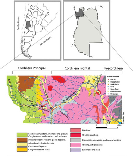
The Argentinean Andes at ~32.5°S are formed by three geological provinces lying in a N–S orientation: the Cordillera Principal to the west, and the Cordillera Frontal and Precordillera to the east. The first constitutes at this latitude the Cordillera de los Andes and the second the Cordillera del Tigre and Cordón del Plata (Corte and Espizúa 1981); the third much lower unit is called the Precordillera (Baldis et al. 1982) (Fig. 1). Mountains at these latitudes have the highest mean elevations in the Andes outside of the Bolivian Altiplano, representing a significant barrier for Pacific air masses, which generate a marked precipitation gradient in the west-to-east direction (Viale and Nuñez 2011). Most of the precipitation in the Cordillera Principal falls in the winter as snow, while the summers are markedly dry (Corripio et al. 2007). Austral winter precipitation of Pacific (west) provenance increases from 300 mm on the Chilean coasts to more than 1000 mm over the windward Chilean slopes (Corte and Espizúa 1981). To the east of the Continental Divide, in the Argentinian sector, precipitation decreases rapidly, reaching 200–500 mm in the Cordillera Principal and less than 50 mm in the Uspallata Valley to the east of the Cordillera Frontal (Hoke et al. 2013).

Figure 1. Map of the study zone and the associated geological characteristics, based on geological map 3369-I, Aconcagua (SEGEMAR 2014). 1: El Salto North Stream; 2: El Salto South Stream; 4: El Salto Stream; 5: Potrerillos precipitation; 6: Mendoza River in Guido; 7: Frontal groundwater spring; 8: Alumbre Stream; 9: Uspallata Stream; 10: Tambillos Stream; 11: San Alberto Stream; 12: Mendoza River; 13: Chacay Stream; 14: Ranchillo Stream; 15: Picheuta Stream; 16: Cortaderas Stream; 17: Tambillos Stream; 18: Polvaredas Stream; 19: Polvaredas precipitation; 20: Polvareditas Stream; 21: Negro Stream; 22: Colorado River; 23: Mendoza River; 24: Vacas River; 24: Cuevas River; 25: Relincho debris-covered and rock glacier; 26: Tupungato River; 28: Valle Azul snow catchment; 29: Santa María Stream; 30: Los Puquios snow catchment; 31: Cementerio Stream; 32: Cuevas River in Puente del Inca; 33: Puente del Inca precipitation; 34: Horcones River; 35: Horcones precipitation; 36: Almacenes rock glacier; 37: Horcones River in Durazno Ravine; 38: Horcones Inferior debris-covered glacier; 39: Horcones Superior Glacier; 40: Cascada Blanca Spring; 41: La Salada Spring; 42: unnamed spring (near Vertiente del Inca); 43: Tolosa Rock Glacier; 44: sample U5; 45: Cuevas River in Las Cuevas village; 46: Cuevas River in Matienzo Ravine; 47: Bonete Stream; 48: Matienzo debris-covered and rock glacier; 49: Alma Blanca Glacier; 50: Piloto Glacier.

In the austral summer, precipitation close to 150–200 mm in northern Mendoza is associated with synoptic convective storms. Summer precipitation is linked to northerly and easterly low-level winds that carry moisture from Atlantic and Amazon source regions. Precipitation that originates from the east only penetrates as far as the Cordillera Frontal, rarely reaching the Cordillera Principal (Hoke et al. 2013).

2.1.1 Geological setting

Non-volcanic Quaternary deposits affected by seismic activity characterize the Andes between 28°S and 33°S. At these latitudes, Aconcagua is the highest peak, with an elevation of 6960.8 m a.s.l. (IGN 2012). Volcanic rocks and marine clastic and evaporitic sediments (gypsum and calcareous deposits) dominate in the Cordillera Principal (Ramos et al. 1996). Glacial deposits from at least four different glaciations during the Pliocene and Quaternary eras are widespread in the main valleys (Ramos et al. 2000). The Cordillera Frontal includes Paleozoic–Triassic andesitic to silicic magmatic rocks of the Choiyoi Group (Caminos 1979). The Cordón del Plata, as part of the Cordillera Frontal, includes Tertiary continental formations containing gypsum and anhydrite (Folguera et al. 2004). Bordering the Cordillera Frontal, the Precordillera forms the foothills of the Andes between 29°S and 33°S. It is a fold-and-thrust belt developed on a Palaeozoic carbonate platform (Baldis et al. 1982). The main river valleys are formed by unconsolidated alluvial and colluvial Quaternary sediments with abundant gravels and sands. Thermal waters are known at Puente del Inca (2740 m) in the Cordillera Principal (Corti 1924, 2009) (Fig. 1).

2.2 Sampling

The upper part of the Mendoza River basin covers 8034 km² (IANIGLA-ING 2012a). Streams originating as high as 6960.8 m a.s.l. are collected by different tributaries of the Mendoza River (Fig. 1). Most of the streams and small rivers contributing to the Mendoza River in the upper basin were sampled, including those located in the Cordón del Plata–Cordillera del Tigre areas. In addition to streamflows, a variety of ice bodies were sampled at the outflow stream from the snout of the glacier (Table 1 and Fig. 1).

Table 1. Sampling design. Mix. Ppal-Ftal: samples taken in the Mendoza River where it receives water from both the Cordillera Principal and the Cordillera Frontal. Gl: uncovered glacier; DebCov: debris-covered glacier; Rock gl: rock glacier; Cov&Rock gl: crioform composed of both debris-covered and rock glacier. This classification is according to IANIGLA-ING (2012a).

Geological province	Water sample	Number of sites	Number of samples
Cordillera Principal	Streams	17	72
	Ice bodies: 3 Gl, 1 DebCov, 2 Cov& Rock gl and 2 Rock gl.	8	25
	Groundwater	5	15
	Precipitation	2	11
Cordillera Frontal	Streams	19	98
	Rock glacier	2	7
	Groundwater	1	4
	Precipitation	1	4
Mix. Ppal-Ftal	River	2	14
Precordillera	Precipitation	1	2
	Groundwater	3	7

In total, 259 samples were obtained at 61 sites. The sampling design included precipitation, groundwater, ice bodies, snow catchments and river water from most tributaries to the Mendoza River. The samples were taken in all seasons: summer, autumn, winter and spring, and were collected every three months from summer 2011 to spring 2012. Precipitation samples were collected in Puente del Inca, Polvaredas, Potrerillos and Horcones. We selected these sites because we believe they are representative of most precipitation received in the Cordillera Principal (Puente del Inca and Horcones) and Frontal (Polvaredas). Samples were collected in PVC tubes (2.5 cm diameter, 1 m length), with a wide funnel, and the tubes were covered with light oil to prevent evaporation.

Additional samples representing ice bodies and springs were collected during winter (when it was possible to access the sites; high-elevation sites in the Aconcagua Provincial Park, far from the road, are closed during winter), spring, autumn and summer. In order to characterize water sources from different ice bodies, we considered streams originating at the snout of the various ice bodies identified in the National Glacier Inventory (IANIGLA-ING 2012a, 2012b, 2012c, 2012d), collected in summer, as representatives of each glacier type. We considered the February sampling as a “pure” glacier signature, because the snow in the region, and particularly around the glaciers, had already melted by the middle of December in 2010 and by the end of December in 2011 (personal field observation and Modis mod10a1 daily satellite imagery). Electrical conductivity and temperature were measured in situ with a Sension5 Hach conductivity meter. Samples were collected in 15 mL high-density plastic centrifuge tubes and in 1 L high-density plastic bottles, refrigerated in the field and kept frozen at −12°C until they were shipped to the laboratory for analysis. Samples were sealed with parafilm to prevent evaporation during shipping.

2.3 Chemical and isotopic analysis

Samples from ice bodies and precipitation were analysed for their ionic concentrations in the Laboratory of Radiochemistry and Environmental Chemistry of the Paul Scherrer Institut (PSI), Villigen, Switzerland, using ion chromatography (Metrohm 850 Professional). These samples were analysed for the major ions sulphate, chloride, calcium, magnesium, sodium and potassium, and the detection limits were 1 ppb, 0.6 ppb, 0.9 ppb, 0.4 ppb, 0.4 ppb and 0.8 ppb, respectively.

Due to elevated salt concentration of river waters, stream samples obtained after August 2011 were analysed for major ions following the standard methods of the APHA (American Public Health Association), AWWA (American Water Works Association) and WPCF (Water Pollution Control Federation) (1995), using a flame spectrometry method (for K⁺, Na⁺), a gravimetric method (for SO₄²⁻) and a titration method (for Cl⁻, HCO₃⁻, Ca²⁺ and Mg²⁺) at Laboratorio de Servicios Agrarios y Forestales, Neuquén, Argentina (LASAF).

A wavelength-scanned cavity ringdown spectrometer (Picarro L2130-I) was used to analyse stable isotopes of water in the PSI laboratory. The analytical uncertainty of δ¹⁸O and δ²H was 0.1‰ and 0.5‰, respectively. The standardization was based on Vienna Standard Mean Ocean Water (VSMOW).

2.4 Altitude analysis

Mean basin altitudes associated with each sampling site were estimated using QGIS software (QGIS Development Team 2014) and ice body sizes were provided by the National Glacier Inventory. The significance of the elevation was calculated using a mixed-effects model (nlme package, Pinheiro et al. 2013). The altitude, season and water source were considered as fixed-effect factors, whereas the sampling sites were considered as a random-effect factor to avoid pseudo-replication due to repeated measurements at the same site (Crawley 2007, Zuur et al. 2009). A multi-model inference (package MuMIn, version 1.9.5, Barton 2013) was subsequently conducted to select the best model according to the “Akaike weights” (w_i), based on the Akaike information criterion for small sample sizes (AICc; Burnham and Anderson 2002).

2.5 Statistical analysis of ion concentration and stable isotope signatures of water

In order to characterize the different catchments and sources, the ion concentrations (Figs. 2 and 3) from all samples were analysed using descriptive statistics (see Supplementary Tables S3 and S4) and Piper diagrams (Fig. 4). Also, as a first exploratory analysis, principal component analysis (PCA; package FactoMineR 1.27, Husson et al. 2014) was applied to ion concentration and stable isotope data to identify the main sources of variation (see Section 3.3). To determine the significance of the variables mostly related to the two main axes of variation identified in the PCA analysis (electrical conductivity and δ¹⁸O), a linear mixed-effects model and a multi-model inference were conducted. We selected the best model as explained in Section 2.4, but, in this case, mountain range and season were considered as fixed-effect factors and sampling site as a random-effect factor. For samples from the Cordillera Principal, an additional analysis was conducted considering the hydrological origin and season as fixed-effect factors and sampling site as a random-effect factor. All the statistical analyses in this study were performed in the R statistical environment (R Core Team 2013).

Figure 2. Boxplots of the major ions, pH and electrical conductivity for each season in the Cordillera Principal rivers.

Figure 3. Boxplots of the major ions, pH and electrical conductivity for each season in the Cordillera Frontal rivers.

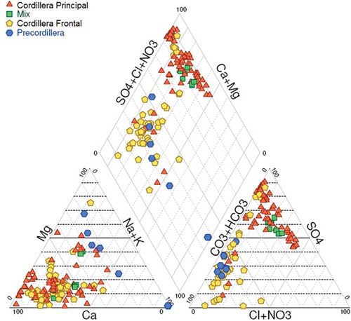
Figure 4. Piper diagram showing differences in ionic composition between samples from the different geological provinces. Chemical compositions of surface and groundwater in the Upper Mendoza River basin vary from calcium sulphate type in the Cordillera Principal to calcium-magnesium bicarbonate type in the Cordillera Frontal and Precordillera.

3 Results

3.1 Ionic characterization of streams

The chemical composition of waters in the Upper Mendoza River basin varies from higher salinities and a dominant water type composed of calcium sulphate in the Cordillera Principal (Figs. 2 and 4) to a lower salinity and a calcium-magnesium bicarbonate type in the Cordillera Frontal (Figs. 3 and 4) and Precordillera (Fig. 4). Unexpectedly, a set of samples from the Cordillera Principal (Santa María and Los Puquios streams) also reveals a calcium bicarbonate composition (Fig. 4). The catchments of these streams drain areas of igneous and granite materials with continental deposits (Fig. 1, points 29 and 30, respectively). There are likewise a few samples from Cordillera Frontal with a calcium sulphate composition, which could have originated in streams from the Cordón del Plata that drain fluvial formations with gypsum, conglomerates and sandstones (Folguera et al. 2004).

The mean composition of the Mendoza River (indicated as “MIX” in Fig. 4) is closer to the hydrochemical composition of the Cordillera Principal, which contains higher altitude catchments with both higher glacier cover and higher outcrops of evaporite marine deposits (gypsum).

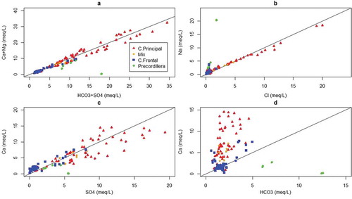
The plot of Ca²⁺ + Mg²⁺ versus SO₄²⁻ + HCO₃⁻ (Fig. 5(a)) from the Cordillera Principal and the Cordillera Frontal shows most of the river water samples lie close to the 1:1 line, indicating that dissolutions of calcite, dolomite and gypsum are the dominant reactions in the system. Na⁺/Cl⁻ and Ca²⁺/SO₄²⁻ correlations in waters from the Cordillera Principal and Frontal (Fig. 5(b,c)) indicate that halite and gypsum dissolution from evaporitic sequences are the main processes affecting stream water chemistry. Similar dissolution of continental deposits with gypsum may act in the Cordón del Plata area (Cordillera Frontal). Most samples from the Cordillera Frontal and groundwater from the Precordillera have Na⁺/Cl⁻ ratios greater than 1, interpreted as Na⁺ released from a silicate weathering reaction (Meybeck 1987). Furthermore, HCO₃⁻ is the dominant anion in waters from the Cordillera Frontal and Precordillera (Fig. 4), according to the reaction of calcite and silicate minerals with carbonic acid in the presence of water (Elango et al. 2003).

Figure 5. Plots of (a) Ca²⁺+Mg²⁺ and SO₄^2-+HCO₃⁻, (b) Na⁺ and Cl⁻, (c) Ca²⁺ and SO₄²⁻ and (d) Ca²⁺ and HCO₃⁻, explaining the dissolution processes. The lines represent the 1:1 relationship.

3.2 Stable isotopes of water

Considering all stream samples, there is a clear difference in the stable isotope signature of water from different geological provinces (see Supplementary Excel data). The δ¹⁸O and δ²H values are more depleted, with less widely spread values in the Cordillera Principal than in the Cordillera Frontal (Figs. 6, 7 and 8).

Figure 6. Boxplots of δ¹⁸O for the waters draining each geological province and the waters of a mixture coming from the Cordillera Principal and the Cordillera Frontal (Principal-Frontal). δ²H shows the same response.

Figure 7. Boxplots of δ¹⁸O, δ²H and deuterium excess for the rivers from the Upper Mendoza River basin and the δ¹⁸O signature for the Cordillera Principal, Cordillera Frontal and the mix of water from both geological provinces, represented in each season.

Figure 8. Scatterplot of stable isotope values for all the samples analysed. The grey line represents the LMWL obtained from Hoke et al. (2013) data and our precipitation samples (δ²H = 8.29 δ¹⁸O + 13.13, R² = 0.99). The black line shows the global meteoric water line (Craig 1961).

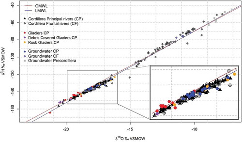
Stable isotope values of precipitation were used to calculate a local meteoric water line, which was slightly different from that reported in Hoke et al. (2013) for the same area (δD = 8.29δ¹⁸O + 11.75, R² = 0.98; this study: δD = 8.29δ¹⁸O + 13.13, R² = 0.99). All samples plot near Craig’s global meteoric water line (GMWL) (Fig. 8).

Because of the high variability in stable isotope signatures of water observed in the Cordillera Frontal, due to the contributions of both Atlantic summer and Pacific winter precipitation, we analysed the signatures of different water sources only in the Cordillera Principal geological province.

The most depleted values (lower δ¹⁸O and δ²H) were observed in glaciers (uncovered and covered), with groundwater and rock glaciers, followed by increasing δ¹⁸O values. Snow values overlap with the signatures of other water sources, including groundwater, showing highly variable values (Fig. 9).

Figure 9. Boxplot of δ¹⁸O for the different water sources analysed in the Cordillera Principal. gl: uncovered glacier; glCov: debris-covered glacier; Rgl: rock glacier; and glCov&Rgl: crioform composed of both debris-covered and rock glacier.

3.3 PCA analysis

The two main dimensions retained by the PCA for the Cordillera Principal and the Cordillera Frontal were associated with the ionic and stable isotope chemistry. The first dimension explained 44.02% of the variability, and was associated with electrical conductivity (EC) and ionic chemistry; while the second dimension explained 17.21% of the variability, and was associated with stable isotope composition (δ¹⁸O, δ²H and d-excess or “Dex”) (Fig. 10(a)). For the analysis of the Cordillera Principal water sources (Fig. 10(b)), the results were similar, with 37.39% of the variability explained by the first dimension (best correlated with EC), and 21.73% of the variability explained by the second dimension (best correlated with the stable isotopes of water). Figure 11 indicates that the first dimension, related to ionic chemistry, clearly separates groundwater and ice bodies, while the second dimension separates the different ice bodies (rock glaciers and debris-covered + uncovered glaciers). See the Supplementary material, Figure S1, which shows a dispersion plot of δ¹⁸O and EC for the different water sources.

Figure 10. PCA plots for (a) the Upper Mendoza River basin and (b) the Cordillera Principal geological province. The main variables affecting the two leading dimensions of the principal components analysis are EC and δ¹⁸O.

Figure 11. Temporal evolution of stream waters and positions of the different water sources along the principal component axes (PC) for the main streams and sources in the Cordillera Principal. (a) Cuevas River in Puente del Inca, (b) La Salada Spring, (c) Horcones River, (d) Vertiente del Inca Spring, (e) Tupungato River in Punta de Vacas, (f) Tolosa Rock Glacier, (g) Cuevas River in Punta de Vacas, (h) Vacas River in Punta de Vacas, (i) Cuevas River near the Matienzo Valley, (j) Santa María Stream, (k) Valle Azul Stream*, (o) Los Puquios Stream, (p) Horcones Inferior debris-covered glacier, (q) Horcones Superior uncovered glacier, (r) unnamed spring (near Vertiente del Inca), and (u) temporal spring in Las Cuevas. Water samples collected in different seasons, beginning in summer 2011, continuing in autumn, winter, spring and summer 2012 are marked as 1, 2, 3, 4 and 5, respectively, after the identification character. Each line points in the direction of time, starting in summer 2011 and ending in summer 2012. Triangles and squares: groundwater; blue stars: uncovered and debris-covered glaciers; brown stars: rock glaciers. * snow-derived stream, only active in spring.

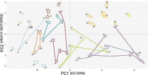
The temporal evolution of different streams along the main PCA dimensions, marked in Figure 11, showed movement along the stable isotope axis (dimension 2), which in summer was remarkably distinct from the other seasons in several rivers (Vacas, Cuevas, Tupungato, Horcones). Changes from autumn to spring were observed mainly in the ionic chemistry dimension (dimension 1). Based on these results, and the hypothesized differences among mountain ranges and sources, we ran mixed-effects models for two variables that were best correlated with the two dimensions EC and δ¹⁸O (see next section). In addition, Figure S2 (Supplementary material) shows a boxplot of the δ¹⁸O evolution for the main tributaries of the Mendoza River in the Cordillera Principal (Tupungato, Cuevas and Vacas rivers), and also the Mendoza River in different locations, in a west-to-east transect.

3.4 General linear mixed-effects model (GLMM) for electrical conductivity

3.4.1 EC and mountain ranges

The generalized linear mixed-effects model for the variable EC indicates significant differences between the two main mountain ranges and among sampling seasons, with higher conductivities for the Cordillera Principal (mean: 1369 µS/cm) than the Cordillera Frontal (mean 393 µS/cm), and in winter–autumn than summer or spring (Figs. 2, 3; see also Table S4 in the Supplementary material).

Using the multi-model inference to compare different models of EC, including combinations of the fixed factors (season and mountain range), the model that includes both factors gave the best results, with an Akaike weight of 1 (R² = 0.76). The Cordillera Principal (intercept) is statistically different from the Cordillera Frontal (p < 0.001), but it cannot be distinguished from waters that are a mix of both mountain ranges (Mix. Ppal-Ftal). The difference between summer and winter–autumn was also significant (Table 2).

Table 2. Mean (x), standard deviation (SD) and confidence range (CR) relative to the intercept value of geological provinces and season, in comparison with the intercept (Cordillera Principal and summer). The significance of statistical tests illustrates the differences between the electrical conductivity (EC) of water derived from the Cordillera Principal and the Cordillera Frontal, and between the summer and other seasons. Mix. Ppal-Ftal: samples taken in the Mendoza River where it has a mixture of waters coming from the Cordillera Principal and the Cordillera Frontal. The significance factors are: p < 0.001 (***), 0.01 (**), 0.05 (*) and 0.1 (.).

Variable	x	SD	CR (2.5–97.5%)	p
(Intercept)	1522.7	173.9	1181.80; 1863.63	<2 × 10^−^16	***
Mix. Ppal-Ftal	907.4	632.2	−1854.5; 623.88	0.330
Cordillera Frontal	278.2	260.8	−1755.66; −733.27	0.000	***
Autumn	1798.7	69.1	139.95; 413.19	0.000	***
Winter	1710.3	57	75.94; 299.27	0.001	***
Spring	1519.7	65.3	−130.93; 125.01	0.964

3.4.2 EC in different sources of the Cordillera Principal

The models performed with data from the Cordillera Principal indicate differences among ice bodies and groundwater, in addition to the seasonal differences. Uncovered glaciers and snow catchment streams show the lowest values, with mean values around 32 µS/cm and 159 µS/cm, respectively. Debris-covered and rock glaciers show an average EC of 805 µS/cm and 12 001 µS/cm, respectively. Finally, groundwater presents the highest average, with a value of 2667 µS/cm, and streams show an intermediate value of 1291 µS/cm (Table S4).

Using the multi-model inference to compare different models of EC, including combinations of the fixed factors (season and source), the model that includes both factors resulted in the best model, with an Akaike weight of 1 (R² = 0.75).

The intercept (uncovered glacier and summer) is statistically different from groundwater (p < 0.05), but it cannot be distinguished from waters from debris-covered glaciers, rock glaciers and rivers/streams. The difference between summer and winter−autumn seasons was also significant (Table 3), but summer was not different from spring.

Table 3. Mean (x), standard deviation (SD) and confidence range (CR) relative to the intercept value of water source and season in the Cordillera Principal, in comparison with the intercept (uncovered glacier and summer). The significance of statistical tests illustrates the differences between EC from uncovered glaciers in contrast with the other water sources, and between the summer (intercept) and the other seasons. Refer to Table 2 for significance factor explanation.

Variable	x	SD	CR (2.5–97.5%)	p
(Intercept)	101.7	987	−1832.86; 2036.19	0.917
Autumn	669.3	148.2	277.20; 858.03	0.000	***
Winter	406.6	125.8	58.40; 551.38	0.015	*
Spring	17.9	140.8	−359.78; 192.13	0.552
Debris-covered glacier	779.5	1438.3	−2141.28; 3496.95	0.637
Rock glacier	1240.9	1083	−983.52; 3261.84	0.293
Rivers and streams	1177.6	1022.1	−927.29; 3079.09	0.293
Groundwater	2466.9	1095.7	217.62; 4512.80	0.031	*

3.5 GLMM of stable isotopes of water

3.5.1 Mountain ranges

A mixed-effects model (nlme package, Pinheiro et al. 2013) was conducted, including different combinations of fixed effects, with δ¹⁸O as a response variable. We considered mountain range and season as fixed-effect factors and sampling site as a random-effect factor in order to prevent temporal pseudo-replication due to repeated measurements at the same site (Crawley 2007). To select statistically relevant predictor variables, a multi-model inference (package MuMIn, version 1.9.5, Barton 2013) was conducted to select the best model according to the Akaike weights (w_i) based on the Aikaike information criterion for small sample sizes (AICc; Burnham and Anderson 2002) (Tables 4 and 5). The best model, with wi=1, was the model that included both geological province (GP) and season (S) as fixed effect factors (Table 4). Similar results were obtained for models with δ²H and d-excess as response variables.

Table 4. Akaike weights (w_i), according to the number of parameters and ΔAICc from the different models. GP: geological province; S: season.

Model	Fixed-effect factors	df	AICc	ΔAICc	wi	R^2
4	GP+S	9	790	0	1	0.88
2	GP	6	810.3	20.32	0	0.86
3	S	6	878.7	88.77	0	0.83
1	Null model	3	895.4	105.41	0	0.81

The Cordillera Principal is statistically different from the Cordillera Frontal (p < 0.001), but its waters cannot be distinguished from waters that are a mix of both mountain ranges (Table 5 and Figs. 6 and 7).

Table 5. Mean (x), standard deviation (SD) and confidence range (CR) relative to the intercept value of geological provinces and season in comparison with the intercept (Cordillera Principal and summer). The significance of statistical tests illustrates the differences between the δ¹⁸O signatures from water derived from the Cordillera Principal (intercept) in contrast with waters from the Cordillera Frontal and Precordillera, and between the summer (intercept) and the other seasons, for n = 229 observations. Mix. Ppal-Ftal: samples taken in the Mendoza River where it has a mixture of waters coming from the Cordillera Principal and the Cordillera Frontal. Refer to Table 2 for significance factor explanation.

Variable	x	SD	CR (2.5–97.5%)	p
(Intercept)	−18.07	0.37	−18.8; −17.35	<2 × 10^−^16
Mix. Ppal-Ftal	−17.22	1.47	−2.04; 3.73	0.5654
Cordillera Frontal	−13.12	0.57	3.824; 6.07	<2 × 10^−^16	***
Precordillera	−7.35	0.9	8.92; 12.46	<2 × 10^−^16	***
Autumn	−18.64	0.16	−0.86; −0.25	0.0005	***
Winter	−18.95	0.16	−1.15; −0.51	0.0000	***
Spring	−18.94	0.18	−1.14; −0.42	0.0000	***

3.5.2 Water sources in the Cordillera Principal

When performing the multi-model inference to select statistically relevant predictor variables, according to the AIC, altitude was not significant (Table 6). For that reason we eliminated this variable from the analysis that follows and performed the multi-model inference without altitude. See also Figure S2 in the Supplementary material.

Table 6. Akaike weights (w_i) according to the number of parameters and ΔAICc from the different models, using as fixed-effect factors the variables water source (source), season and altitude, for the Cordillera Principal geological province.

Model	Fixed-effect factor	df	AICc	ΔAICc	wi
5	Source	10	446.9	0	0.641
7	Season+source	13	448.1	1.18	0.355
8	Altitude+season+source	14	457.5	10.65	0.003
6	Altitude+source	11	459.3	12.37	0.001
4	Altitude+season	7	467.6	20.69	0
2	Altitude	4	467.8	20.88	0
1	Null model	3	474.8	27.95	0
3	Season	6	477.2	30.31	0

For the different models in this mountain range, including season and source as fixed factors, the best model (Model 3 in Table 7) includes only the fixed factor source, with a weight of 0.717. According to these models, the hydrological origin (variable “source”) of water in the Cordillera Principal had a significant effect on δ¹⁸O, δ²H and d-excess values (Tables 7, 8 and 9). The difference is clear among glaciers and the rest of the water sources (Table 8).

Table 7. Akaike weights (w_i), according to the number of parameters and ΔAICc from the different models, using as fixed-effect factor the variables water source (source) and season, for the Cordillera Principal geological province.

Model	Fixed-effect factor	df	AICc	ΔAICc	wi	R^2
3	Source	10	459.3	0	0.72	0.39
2	Source+season	13	461.2	1.86	0.28	0.42
4	Null model	3	491.7	32.43	0	0.17
1	Season	6	495.3	36.01	0	0.2

Table 8. Mean (x), standard deviation (SD) and confidence range (CR), relative to the intercept value, of water sources and seasons in comparison with the intercept (uncovered glacier and summer). The significance of statistical tests illustrates the differences between the δ¹⁸O signatures from uncovered glaciers (intercept) and the other water sources, and between the summer (intercept) and the other seasons, for 125 observations in the Cordillera Principal geological province. Refer to Table 2 for significance factor explanation.

Variable	x	SD	CR (2.5–97.5%)	p
(Intercept)	−19.37	0.46	−20.27; −18.47	<2 × 10^−^16	***
Debris-covered glacier	−20.2	0.92	−2.63; 0.97	0.366
Debris-covered and rock glacier	−20.45	0.86	−2.78; 0.60	0.208
Total precipitation	−14.35	0.89	3.27; 6.76	<2 × 10^−^16	***
Rock glacier	−17.3	0.89	0.32; 3.82	0.020	*
Rivers and streams	−18.01	0.56	0.27; 2.45	0.015	*
Snow	−15.12	0.87	2.54; 5.96	0.000	***
Groundwater	−17.67	0.65	0.42; 2.98	0.009	**
Autumn	−19.91	0.37	−1.27; 0.19	0.149
Winter	−20.2	0.39	−1.61; −0.05	0.037	*
Spring	−20.28	0.45	−1.79; −0.03	0.042	*

The statistical significance of the different sources is variable. Uncovered glaciers (intercept) and debris-covered glaciers were not significantly different. Uncovered glaciers showed a significant difference from rock glaciers and rivers/streams (p < 0.05), and groundwater (p < 0.01).

The highest significance level is observed for total precipitation and snow samples, reaching p < 0.001 (Table 8). However, because there are only a few samples with high stable isotope variability, this result may not adequately represent the entire spatial and temporal spectrum of variation in precipitation.

When the analysis was conducted for deuterium excess (Table 9), it was possible to identify a significant distinction between the uncovered glaciers (intercept) and the solely snow-covered catchments (Valle Azul and Los Puquios basins). The difference from groundwater and rivers/streams (which represent a mix from different water sources) samples was also significant.

Table 9. Mean (x), standard deviation (SD) and confidence range (CR) relative to the intercept value of water source and season in comparison with the intercept (uncovered glacier and summer). The significance of statistical tests illustrates the differences between the deuterium excess values from uncovered glaciers (intercept) and the other water sources, and between the summer (intercept) and the other seasons, for 125 observations in the Cordillera Principal geological province. Refer to Table 2 for significance factor explanation.

Variable	x	SD	CR (2.5–97.5%)	p
(Intercept)	9.67	0.78	8.14; 11.20	<2 × 10^−^16	***
Autumn	10.36	0.71	0.079; 2.25	0.3339
Winter	10.49	0.82	0.23; 2.54	0.3154
Spring	10.12	0.67	−0.66; 2.17	0.5046
Debris-covered glacier	10.16	1.57	−2.59; 3.57	0.7546
Debris-covered and rock glacier	7.39	1.49	−5.2; 0.62	0.1252
Total precipitation	8.89	1.43	−3.58; 2.03	0.5875
Rock glaciers	6.95	1.43	−5.51; 0.06	0.0567	.
Rivers and streams	7.25	0.94	−4.24; −0.6	0.0098	**
Valle Azul basin	6	1.84	−7.28; −0.08	0.0462	*
Snow	9.78	1.52	−2.88; 3.099	0.9437
Los Puquios basin	6.75	1.39	−5.64; −0.2	0.0363	*
Groundwater	7.28	1.11	−4.56; −0.24	0.0303	*

4 Discussion

4.1 Differentiation of mountain ranges

The Cordillera Principal and the Cordillera Frontal presented clear differences in ionic and stable isotope chemistry, which could potentially be used in further work to quantify the contributions of each mountain range to the flow of the Mendoza River. As explained in Hoke et al. (2013), the lower and less variable natural abundance of δ¹⁸O and δ²H in the Cordillera Principal can be explained by their different moisture sources, which, for the Cordillera Principal, are almost exclusively the Pacific Ocean and winter precipitation, and for the Cordillera Frontal, both the Pacific (winter) and Atlantic (summer) oceans. Differences in EC between the two mountain ranges are related to geological controls (higher water salinity in the Cordillera Principal due to dissolution of evaporitic deposits), as was observed in the Tunuyán River basin (León and Pedrozo 2014), situated in the south of our study area. Our study indicates that ionic chemistry could be used as an additional tracer of the geographic origin of river water, because the different geological settings are reflected in a stream’s chemistry. The Mendoza River trunk, near the Potrerillos Dam, has ionic and stable isotope chemistry closer to that of the Cordillera Principal streams (Figs. 4 (Mix) and 8 (Principal–Frontal)), indicating a higher contribution by this mountain range.

When the altitude effect in isotopic signatures was calculated through the GLMM, using altitude, season and mountain range as fixed-effect factors and sampling site as random-effect factor, the best model included the three fixed-effect factors with an Akaike weight of w_i = 0.81 (Table 10). However, moisture source had a stronger effect than altitude (Table 11; altitude: p < 0.1; geological province, Cordillera Frontal: p < 0.05; seasonality: p < 0.001). When precipitation at different altitudes originates from different air masses, altitude effects cannot be calculated, because the origin of air masses often has a greater influence on the isotopic signals than the well-known “altitude effect” (Rank and Papesch 2005). The Cordillera Principal has higher altitude peaks than the Cordillera Frontal, and the sources of precipitation for each range are different. For these reasons, we did not attempt to calculate altitude effects in the regional analysis of mountain ranges, in order to avoid autocorrelation between mountain range and altitude.

Table 10. Akaike weights (w_i) according to the number of parameters and ΔAICc from the different models. GP: geological province.

Fixed-effect factors	df	AICc	ΔAICc	wi	R^2
Altitude+GP+season	9	583.14	0	0.81	0.88
GP+season	8	586.15	3.01	0.18	0.87
Altitude+season	7	591.09	7.95	0.02	0.87
Season	6	609.47	26.33	0	0.85
Altitude+GP	6	615.46	32.32	0	0.85
GP	5	617.23	34.1	0	0.83
Altitude	4	622.96	39.82	0	0.84
(Null model)	3	639.84	56.71	0	0.81

Table 11. Mean (x), standard deviation (SD) and significance of geological province, season and altitude fixed-effect factors in comparison with the intercept (Cordillera Principal and summer). The significance of statistical tests illustrates the differences between the δ¹⁸O signatures of water derived from the Cordillera Principal (intercept) and the Cordillera Frontal geological provinces and between the summer (intercept) and the other seasons. Mix. Ppal-Ftal: samples taken in the Mendoza River where it has a mixture of waters coming from the Cordillera Principal and the Cordillera Frontal. Refer to Table 2 for significance factor explanation.

Variable	x	SD	p
(Intercept)	−8.17	4.87	0.09	.
Altitude	−8.17	0.00	0.06	.
Mix. Ppal-Ftal	−8.47	1.46	0.84
Cordillera Frontal	−5.75	1.14	0.03	*
Autumn	−8.92	0.18	0.00	***
Winter	−9.24	0.17	<2 × 10^−^16	***
Spring	−9.37	0.20	<2 × 10^−16	***

4.2 Differentiation of sources in the Cordillera Principal

Stable isotope compositions in different water sources are affected by land–atmosphere exchange processes, such as precipitation, evaporation and sublimation (Kendall and McDonnell 1998), which change according to altitude, temperature, stable isotope composition of source water vapour, and surface characteristics that affect the energy balance and the evaporation/sublimation processes (e.g. sediment type and its distribution in glaciers affects albedo, absorbed radiation, melting and evaporation). Quite differently, the ionic chemistry of waters is affected by water–sediment dissolution, reflecting contact time between waters and sediments, the mineral composition of different basin areas, and chemical evolution of waters along their course.

Although several studies have found altitude effects in δ¹⁸O from precipitation, e.g. −0.17/–0.2‰ per 100 m in the Alps (Siegenthaler and Oeschger 1980, Schotterer et al. 1997, Poage and Chamberlain 2001, Windhorst et al. 2013, Mariani et al. 2014), −0.1‰ per 100 m in springs from Italy (Bono et al. 2005), and −0.6 and −1.0‰ per 100 m for snow samples in the South American Andes (Niewodniczanski et al. 1981), the slope of the altitude effect is variable, depending on temperature and the associated isotope fractionation during condensation, altitude, orographic characteristics, source moisture (Horvatinčić et al. 2005) and air mass trajectories (Aouad-Rizk et al. 2005). In the Cordillera Principal, stable isotope values were better explained by source waters and seasonal variations, probably related to shifts in the relative contribution of different water sources to the streams (Table 6). In the Cordillera Principal, isotope effects given by “rain out” may be more important on the windward side of the mountains, in Chile. On the leeward eastern slopes, altitudes decrease while air masses move east, so other factors may have more influence on isotope signals, such as the relative contribution of different ice bodies. Post-depositional changes in snow related to weather and topography (Niewodniczanski et al. 1981, Poage and Chamberlain 2001) have been proposed as factors that can alter or even invert the altitude effect on stable isotopes.

Stable isotope values presented clear differences for ice bodies, such as uncovered and debris-covered glaciers versus rock glaciers (Table 8), while electrical conductivity (Table 3) was significantly different only between groundwater and uncovered glaciers, with intermediate values for the other ice bodies (debris-covered glaciers and rock glaciers). The most depleted waters (i.e. lower amount of heavy isotopes) originated from debris-covered glaciers, while the most enriched waters (i.e. higher abundance of heavy isotopes) originated from rock glaciers (Table 8). In our study, debris-covered and uncovered glaciers have a similar glacigenic origin, while rock glaciers have a cryogenic origin. Rock glaciers form from subsequent snow avalanches, where debris falls from mountain slopes, generating a variable content of rock and ice (40–60%) (Brenning 2003). This causes a gravitational movement, as in plastic materials, which forms ridges and gullies that facilitate snow accumulation. Water in these ice bodies is subjected to melting on the surface, infiltration, contact with rocks and sediments, and refreezing in the depth of the ice body, which may explain the higher isotope enrichment and ionic concentration compared to that present in the other ice bodies (Table 8).

Groundwater had intermediate isotope values between rock glaciers and uncovered glaciers, probably because they originate from a combination of sources and represent longer time scales. Stable isotope composition of snow had high variability, overlapping with values of groundwater and ice bodies, most likely related to the high spatial and temporal isotopic variability of snow, which can be evident even during a storm event (Gat 2010). When performing a deuterium excess analysis it was possible to differentiate snow catchments from ice-dominated basins (Table 9), indicative of extra evaporative processes in snow compared to glaciers.

Moreover, in order to distinguish contributions of snow (in the Cordillera Principal), whose stable isotope values overlap those of other sources, and groundwater, which has intermediate values between different ice bodies, EC or individual ions may be useful. The highest salinities were found in groundwater, reaching 5290 µS/cm (Table S4), probably caused by longer contact times with sediments. Waters from uncovered glaciers and snow-dominated streams presented the lowest salinities, with values of 32–159 µS/cm and 121–377 µS/cm, respectively. In contrast, rock glaciers and debris-covered glaciers from the Cordillera Principal are located in an area with gypsum deposits, so the differences in ionic concentrations are related to the contact time of debris and ice, resulting in higher EC values for rock glaciers than for debris-covered glaciers, with mean values of 1201 µS/cm and 805 µS/cm, respectively (Table S4). A combination of all variables measured, shown in the PCA plot in Figure 11, indicates clear differences along the first dimension related to ionic chemistry. This dimension allows us to separate groundwater from snow and glacially-derived streams. The second dimension, related to stable isotope chemistry, reflects the differences among rock glaciers and the other ice bodies (uncovered and covered glaciers).

Our study shows the main chemical differences among water sources contributing to the Upper Mendoza River basin, suggesting that ionic chemistry and stable isotopes may allow the quantification of the contribution of different sources to a river’s discharge. Based on the temporal evolution of streams in the two main axes of variation (Fig. 11), we propose that such evolution reflects changes of stable isotope and ionic chemistry due to different relative contributions of ice bodies, groundwater and snowmelt water. Samples obtained in the summer are isotopically enriched, which can be explained by isotopic elution (Ohlanders et al. 2013).

The large shift of isotope signatures from summer to autumn, to more depleted values, may be caused by temporal differences in the glacier albedo. Because the snow has already disappeared in the late summer, the albedos of the glaciers are at their minimum values, glacial ablation is at a maximum, increasing glacier melt and relative contributions to the streams. Later, in winter, the isotopic signatures remain relatively constant, probably reflecting glacial and groundwater contributions. A similar pattern was observed for the same period on the Chilean side at the same latitude as our study site (Rodriguez et al. 2014). However, the dilution observed in the ion axis (dimension 1) suggested the contribution of snow, initially depleted in heavy isotopes because of low temperatures. When spring arrives, salt dilution is remarkable, because of a peak of discharge of snowmelt, as was observed in Chile by Ohlanders et al. (2013) and Rodriguez et al. (2014) in the spring season. When the summer progresses, a temporal enrichment of heavy isotopes was observed in these studies due to the above-mentioned isotope elution process (Fig. 11).

Ionic concentrations increased in the autumn for some streams (e.g. Cuevas River in Puente del Inca and Horcones River, Fig. 11), probably reflecting a higher contribution of groundwater. This suggests that groundwater maintains the baseflow of these streams during autumn and winter, and the same feature was also observed on the Chilean side of the mountains (Rodriguez et al. 2014). We note that the springs sampled for this study could represent melting of permafrost, or groundwater derived from fractured aquifers. Further research is needed to understand the dynamics and origin of spring waters in these mountain areas. Other streams, such as Tupungato and Vacas, do not show an important change along the ionic chemistry axis, but move mainly along the isotope axis. All the streams may be reflecting a change, through the isotope axis, in the relative contribution of snow, dominant in early summer, to ice bodies in late summer and autumn, and to groundwater in winter.

The sample u5 (Fig. 11) corresponds to a temporal small lagoon and was analysed to trace its water source. The water source for this little lagoon seems to be related more to snow or rain than to groundwater, especially taking into account the first component, and much more depleted in ions than the rest of the groundwater samples.

5 Conclusion

Ion chemistry and stable isotopes can be used to distinguish different geographic and hydrological origins of water of the Upper Mendoza River basin. We found clear differences in ionic and stable isotope chemistry between the main morphotectonic units of first order, related to different precipitation systems (Pacific and Atlantic moisture sources) and geological settings. Hydrological sources in the Cordillera Principal, such as ice bodies, groundwater, snow catchments and precipitation, also showed differences in ionic and stable isotope chemistry. Stable isotopes indicated different water–atmosphere interactions in ice bodies, showing highest and lowest enrichments in rock and debris-covered glaciers, respectively. Snow-dominated catchments were more evaporated and presented lower deuterium excess values compared with glacier-dominated basins. Ionic chemistry (indicated by EC and ion concentrations) reflected water–sediment interactions, with the highest salt concentrations in groundwater, which has the longest contact times with sediments, and the lowest values in snow and streams dominated by uncovered glaciers. Temporal variability of river water was observed in both ionic and isotope chemistry, showing changes in the relative importance of the contributions of different sources to the rivers in the Cordillera Principal, and pointing to the importance of glaciers and groundwater to the discharge of the Mendoza River.

Acknowledgements

Isabella Mariani helped with isotopic analysis at the PSI, Switzerland, and Hayes Fountain helped with language writing. The Dirección de Recursos Naturales Renovables of Mendoza Province provided permission to deploy collectors, carry out sampling and work with park rangers in protected areas (A. Zalazar, V. Ottero, R. Massarelli, O. Aranibar and J. Gimenez). Alejandro Casteller, Ernesto Corvalán, Federico Gonzalez, Marcelo Quiroga, Gustavo Costa and Mariano Castro collaborated on fieldwork. Amilcar Alvarez from the National Water Institute helped with the water instruments.

Disclosure statement

No potential conflict of interest was reported by the authors.

Supplementary material

Supplemental data for this article can be accessed here.

Additional information

Funding

This work was supported by the Agencia Nacional de Promoción Científica y Tecnológica (ANPCyT) under grant [PICT 2011(2703)], and University of Cuyo under grant [PID (2011-2013 and 2013-2015)].

References

- Aouad-Rizk, A., et al., 2005. Oxygen-18 and deuterium contents over Mount Lebanon related to air mass trajectories and local parameters. In: Isotopic composition of precipitation in the Mediterranean Basin in relation to air circulation patterns and climate. Vienna: IAEA final report 2000–2004, IAEA-TECDOC-1453, 75–82.
- APHA, AWWA, WPCF, 1995. Standard methods for the examination of water and wastewater. Washington, DC: American Public Health Association, 17.
- Baldis, B., et al., 1982. Síntesis evolutiva de la Precordillera Argentina. 5º Congreso Latinoamericano de Geología, Actas, 4, 399–445.
- Barnett, T.P., Adam, J.C., and Lettenmaier, D.P., 2005. Potential impacts of warming climate on water availability in snow-dominated regions. Nature, 438, 303–309. doi:10.1038/nature04141
- Barton, K., 2013. MuMIn: multi-modelinference. R package version 1.9.5. Available from: http://CRAN.R-project.org/package=MuMIn
- Boninsegna, J. and Villalba, R., 2007. Los condicionantes geográficos y climáticos. Documento marco sobre la oferta hídrica en los oasis de riego de Mendoza y San Juan. Secretaría de Ambiente y Desarrollo Sustentable, Fundación e Instituto Torcuato Di Tella.
- Bono, P., et al., 2005. Stable isotopes (δ18O, δ2H) and tritium in precipitation: results and comparison with groundwater perched aquifers in Central Italy. In: Isotopic composition of precipitation in the Mediterranean Basin in relation to air circulation patterns and climate. Vienna: IAEA final report 2000–2004, IAEA-TECDOC-1453, 115–124.
- Bradley, R.S., Keiming, F.T., and Díaz, H., 2004. Projected temperature changes along the American cordillera and the planned GCOS network. Geophysical Research Letters, 31 (16). doi:10.1029/2004GL020229
- Brenning, A., 2003. La importancia de los glaciares de escombros en los sistemas geomorfológicos e hidrológicos de la cordillera de Santiago: fundamentos y primeros resultados. Pontificia Universidad Católica de Chile: Santiago. Revista de Geografía, Norte Grande, 30, 7–22.
- Bruniard, E., 1994. Los regímenes fluviales de alimentación sólida en la República Argentina. Ensayo de elaboración de un modelo hidroclimático de la vertiente oriental de los Andes. Buenos Aires: Academia Nacional de Geografía, 7.
- Burnham, K.P. and Anderson, D.R., 2002. Model selection and multimodel inference: a practical information-theoretic approach. New York: Springer, 2.
- Caminos, R., 1979. Cordillera Frontal. In: J.C.M. Turner, ed. Segundo Simposio de Geología Regional Argentina. Córdoba: Academia Nacional de Ciencias I, 397–453.
- Ciric, A., 2009. ENSO related climate variability recorded in an ice core from Cerro Mercedario, Central Andes. Thesis (PhD). University of Bern.
- Compagnucci, R. and Vargas, W., 1998. Interannual variability of the Cuyo rivers streamflow in the Argentinean Andean mountains and ENSO events. International Journal of Climatology, 18, 1593–1609. doi:10.1002/(SICI)1097-0088(19981130)18:14<1593::AID-JOC327>3.0.CO;2-U
- Corripio, J.G., Purves, R.S., and Rivera, A., 2007. Modelling climate-change impacts on mountain glaciers and water resources in the Central Dry Andes. In: B. Orlove, E. Wiegandt, and B. Luckman, eds. Darkening peaks: glacier retreat, science, and society. Berkeley: University of California Press, 126–135.
- Corte, A. and Espizúa, L., 1981. Inventario de glaciares de la cuenca del río Mendoza. Mendoza: IANIGLA-CONICET, 62.
- Corti, H., 1924. Contribución al estudio de las aguas termo minerales de Puente del Inca. Publicación nro. 1. Buenos Aires, Argentina: Dirección General de Minas, Geología e Hidrología, Ministerio de Agricultura de la Nación.
- Corti, H., 2009. Agua bajo el puente. Química moderna y análisis de aguas minerales. Ciencia Hoy, 19 (109), 37–43.
- Craig, H., 1961. Isotopic variations in meteoric waters. Science, 133, 1702–1703. doi:10.1126/science.133.3465.1702
- Crawley, M.J., 2007. The R book. Chichester: John Wiley and Sons.
- Elango, L., Kannan, R., and Senthil Kumar, M., 2003. Major ion chemistry and identification of hydrogeochemical processes of groundwater in a part of Kancheepuram district, Tamil Nadu, India. Journal of Environmental Geosciences, 10 (4), 157–166. doi:10.1306/eg100403011
- Folguera, A., et al., 2004. Hoja Geológica 3369-15 Potrerillos. Escala 1:100.000. Servicio Geológico Minero Argentino, Instituto de Geología y Recursos Minerales. ISSN 0328–2333. Buenos Aires: Boletín Nº 301, 142.
- Gat, J.R., 2010. Isotope hydrology, a study of the water cycle. Series on environmental science and management. London: Imperial College Press. 6.
- Hoke, G., et al., 2013. Seasonal moisture sources and the isotopic composition of precipitation, rivers and carbonates across the Andes at 32.5-35.5°S. Geochemistry, Geophysics, Geosystems, 14, 962–978. doi:10.1002/ggge.20045
- Horvatinčić, N., et al., 2005. Tritium and stable isotope distribution in the atmosphere at the coastal region of Croatia. IAEA final report 2000-2004: isotopic composition of precipitation in the Mediterranean Basin in relation to air circulation patterns and climate. Vienna: IAEA-TECDOC-1453, 37–50.
- Husson, F., et al., 2014. Multivariate exploratory data analysis and data mining with R. Available from: http://factominer.free.fr
- IANIGLA-ING (Inventario Nacional de Glaciares), 2012a. Subcuenca del río Tupungato, cuenca del río Mendoza, Provincia de Mendoza. IANIGLA-CONICET, Secretaría de Ambiente y Desarrollo Sustentable de la Nación, 52.
- IANIGLA-ING (Inventario Nacional de Glaciares), 2012b. Subcuencas de los ríos de las Cuevas y de las Vacas, cuenca del río Mendoza, Provincia de Mendoza. IANIGLA-CONICET, Secretaría de Ambiente y Desarrollo Sustentable de la Nación, 67.
- IANIGLA-ING (Inventario Nacional de Glaciares), 2012c. Subcuencas de los ríos Blancos y del Cordón del Plata, cuenca del río Mendoza, Provincia de Mendoza, 57.
- IANIGLA-ING (Inventario Nacional de Glaciares), 2012d. Subcuencas del arroyo Uspallata y del sector Cordillera del Tigre, cuenca del río Mendoza, Provincia de Mendoza, 56.
- IGN, 2012. Intituto geográfico nacional. Available from: www.ign.gob.ar/Novedades/NuevaAlturaAconcagua
- INDEC, 2010. National census. Buenos Aires: Instituto nacional de estadística y censos.
- Kendall, C. and McDonnell, J., 1998. Isotope tracers in catchment hydrology. Amsterdam: Elsevier.
- León, J. and Pedrozo, F., 2014. Lithological and hydrological controls on water composition: evaporite dissolution and glacial weathering in the south central Andes of Argentina (33°-34°S). Hydrological Processes. doi:10.1002/hyp.10226
- Mariani, I., et al., 2014. Temperature and precipitation signal in two Alpine ice cores over the period 1961–2001. Climate of the Past, 10, 1093–1108. doi:10.5194/cp-10-1093-2014
- Masiokas, M., et al., 2006. Variaciones de la precipitación nívea en los Andes centrales de Argentina y Chile, 1951-2005: Influencias atmosféricas de gran escala e implicancias para los recursos hídricos en la región. Journal of Climate, 19, 6334–6352. doi:10.1175/JCLI3969.1
- Masiokas, M., et al., 2013. Recent and historic Andean snowpack and streamflow variations and vulnerability to water shortages in Central Western Argentina. In: R.A. Pielke and Hossain, eds. Climate vulnerability: understanding and addressing threats to essential resources. Elsevier, 213–227.
- Meybeck, M., 1987. Global chemical weathering of surface rocks estimated from river dissolved leads. American Journal of Science, 287, 401–428. doi:10.2475/ajs.287.5.401
- Minetti, J., et al., 1986. El régimen de precipitación de San Juan y su entorno. San Juan: CONICET.
- Niewodniczanski, J., et al., 1981. The altitude effect on the isotopic composition of snow in high mountains. Journal of Glaciology, 27, 99–111.
- Ohlanders, N., Rodriguez, M., and Mc Phee, J., 2013. Stable water isotope variation in a Central Andean watershed dominated by glacier and snowmelt. Hydrology and Earth System Sciences, 17, 1035–1050. doi:10.5194/hess-17-1035-2013
- Panarello, H. and Dapeña, C., 1996. Mecanismos de recarga y salinización en las cuencas de los ríos Mendoza y Tunuyán, Mendoza, República Argentina: evidenciados por isótopos ambientales. Memorias del XII Congreso Geológico de Bolivia, Tomo II.
- Pinheiro, J., et al., 2013. Nlme: linear and nonlinear mixed effects models. R Package Version, 3, 1–109.
- Poage, M. and Chamberlain, C.P., 2001. Empirical relationships between elevation and the stable isotope composition of precipitation and surface waters: considerations for studies of paleoelevation change. American Journal of Science, 301, 1–15. doi:10.2475/ajs.301.1.1
- QGIS Development Team, 2014. QGIS geographic information system. Open Source Geospatial Foundation Project. Available from: http://qgis.osgeo.org
- R Core Team, 2013. R: a language and environment for statistical computing. Vienna: R Foundation for Statistical Computing. Available from: http://www.R-project.org
- Ramos, V., et al., 1996. Geología de la Región del Aconcagua, Provincias de San Juan y Mendoza, Anales, Dirección Nacional del Servicio Geológico, 510.
- Ramos, V., Caminos, R., and Cortes, J.M., 2000. Hoja geológica 3369-I Cerro Aconcagua (1:250.000). Buenos Aires: Subsecretaría de Minería de la Nación, Dirección Nacional del Servicio Geológico.
- Rank, D. and Papesch, W., 2005. Isotopic composition of precipitation in Austria in relation to air circulation patterns and climate. In: Isotopic composition of precipitation in the Mediterranean Basin in relation to air circulation patterns and climate. IAEA final report 2000–2004, Vienna: IAEA-TECDOC-1453, 19–35.
- Rodriguez, M., Ohlanders, N., and McPhee, J., 2014. Estimating glacier and snowmelt contributions to streamflow in a Central Andes catchment in Chile using natural tracers. Hydrology and Earth System Sciences, 18, 1–46.
- Schotterer, U., et al., 1997. Isotope records from Mongolian and Alpine ice cores as climate indicators. Climatic Change, 36, 519–530. doi:10.1023/A:1005338427567
- SEGEMAR, 2014. Geologic map 3369-I Mt. Aconcagua. Servicio geológico minero argentino. Available from: www.segemar.gob.ar
- Siegenthaler, U. and Oeschger, H., 1980. Correlation of 18O in precipitation with temperature and altitude. Nature, 285, 314–317. doi:10.1038/285314a0
- Viale, M. and Nuñez, M., 2011. Climatology of winter orographic precipitation over the subtropical Central Andes and associated synoptic and regional characteristics. Journal of Hydrometeorology, 12, 481–507. doi:10.1175/2010JHM1284.1
- Vogel, J.C., Lerman, J.C., and Mook, W.G., 1975. Natural isotopes in surface and groundwater from Argentina. Hydrological Sciences, XX, 203–207.
- WCRP (world climate research programme achievements), 2009. Scientific knowledge for climate adaptation, mitigation and risk management.
- Windhorst, D., et al., 2013. Impact of elevation and weather patterns on the isotopic composition of precipitation in a tropical montane rainforest. Hydrology and Earth System Sciences, 17, 409–419. doi:10.5194/hess-17-409-2013
- Zuur, A.F., et al., 2009. Mixed effects models and extensions in ecology with R. New York: Springer.