Analysis of dam-induced cyclic patterns on river flow dynamics

ABSTRACT

This paper investigates the impact of the Hungry Horse Dam on streamflow dynamics in the South Fork of the Flathead River, Montana, USA. To this end, pre- and post-dam periods of raw and naturalized streamflow data were analysed. Pettitt’s change point analysis indicated a significant change point in streamflow dynamics due to dam construction. Complexities in the pre- and post-dam periods were evaluated by sample and multi-scale entropy analyses, and the entropies of the post-dam period were found to be higher than those of the pre-dam period. Possible reasons for this, unrelated to the natural hydrological cycle caused by the dam, were analysed using wavelet analyses. The wavelet analyses showed a clear change in the phase relationship between precipitation and streamflow. Finally, weak positive trends found in the hydrological variables indicated the effects of human activities (e.g. dam construction). The results also revealed distorted lead times, which can improve the streamflow forecasts for different lead times.

KEYWORDS:

• Hungry Horse Dam
• Pettitt’s analysis
• sample entropy
• multi-scale entropy
• cross-wavelet transform
• wavelet coherence

Editor D. Koutsoyiannis; Associate editor R. van Nooijen

1 Introduction

Increasing water resources control and development have led to significant hydrodynamical and micro-climatological changes in river basins. The impacts on hydrological processes could change streamflow variations and their underlying dynamics. Irregularities in seasonal and inter-annual streamflow variations can also affect river functions and induce serious environmental and ecological problems. Investigating the factors that influence runoff changes has been receiving increasing interest as higher water demands by municipal, industrial and agricultural sectors have already caused tremendous stress on our water resources, in addition to population explosion and its associated effects, e.g. deforestation and water pollution. Therefore, an understanding of hydrological alterations (Poff et al. 2007) by hydraulic structures such as reservoirs and dams is crucial. Yang et al. (2008) analysed the influences of dam construction on hydrological regimes with a range of variability approach, and concluded that management of reservoirs affects the hydrological processes downstream, and construction of dams introduced hydrological alterations. Yu et al. (2014) investigated river dynamics in stations downstream of the Three Gorges Dam and showed that the dam caused average decreases of 25.1%, 16.5% and 1.9% in the Yichang flow, Datong flow and Santiao river stage, respectively.

To characterize the effects of impoundment in a hydrological regime, the range of variability approach (Yang et al. 2008, Zhao et al. 2012) and indicators of hydrological alteration analysis proposed by Richter et al. (1996) have been widely used (Magilligan and Nislow 2005, Hernández-Henríquez et al. 2010, Lu et al. 2014). However, there are some disadvantages related to these methods: (1) it is difficult to meet the requisite sampling criteria proposed by Richter et al. (1996); (2) the number of records that fulfil length-of-record requirements is high; (3) throughflow alteration assessment must be applied using a record of insufficient length; (4) there are difficulties in determining major dam-influencing hydrological alterations with several dams existing on a river (Magilligan and Nislow 2005, Yang et al. 2008). Furthermore, these analyses are based on pre-assigned time scales and, due to their statistical procedures, implementation at multiple time scales is complicated. As Zhou et al. (2012) stated, multiple time scales are important in obtaining a “complete profile of the hydrological process”. To understand hydrological variations affected by dam construction and to profile multi-scale nonlinear properties, knowledge of the complexity of streamflow would be useful.

The complex nature of a system is associated with its entropy, which is a measure of the degree of uncertainty produced within a system: the higher the entropy, the more random and complex a system is. Sample entropy (SampEn) (Richman and Moorman 2000) has been applied to identify nonlinearity and to analyse hydrological time series (Sen 2009, Huang et al. 2011). However, the pre-determined threshold value, r, and the number of dimensions, m, affect the results for SampEn. Further, SampEn does not allow profiling of multi-scale behaviour. The complexity assessment performed over different time scales provides more details on the system dynamics than a single entropy measure obtained at the original time scale. Multi-scale entropy (MSE), introduced by Costa et al. (2002), has been applied to analysis of multi-scale hydrological time series. Li and Zhang (2008) analysed 131 year-long daily flow rates for the Mississippi River using the MSE analysis and found a possible loss in the complexity of the streamflow after the 1940s due to human activities, with significant changes in land cover and land use including soil conservation applications. However, the authors did not analyse whether 1940 is a statistically significant change point; they only roughly divided streamflow data into two subsets, presumably considering that human activities started to increase after that year. Zhou et al. (2012) analysed the effects of reservoirs on flow regimes with the MSE analysis and concluded that the complexity of the upper reaches is greater than of the lower reach before the construction of the reservoirs. Also, these reservoirs greatly increase the complexity of the river dynamics in the East River in China. While Zhang et al. (2012c) found no evidence regarding the influence of the Gezhouba Dam on Yangtze streamflow changes by employing MSE analysis, Huang et al. (2011) attributed the decrease in complexity of flows in the upper reaches of the Yangtze River to changed land use influenced by dam construction. Sen (2009) concluded that complexity loss might have been caused by increased human activities, such as increasing land-crop utilization and urbanization, but Yan et al. (2011) found an increase in the runoff complexity resulting from anthropogenic activities. Since river discharges are the mixed results of many processes, such as groundwater, fast runoff, climate, topographical features and anthropogenic activities including dam construction, drawing a straightforward conclusion that the reason for complexity loss or gain is non-trivial. However, wavelet analysis can be helpful in determining the reason for changed complexity in streamflow. As White et al. (2005) stated, a streamflow regime is controlled by cyclic phenomena from daily (e.g. daily maxima inducing glacial meltwater) to decadal (e.g. the El Niño Southern Oscillation), characterized by variations in periodicities and amplitudes; these could be disrupted by dams, and cycles additional to the natural hydrological regime could be introduced to the river system. To the best of our knowledge, there is no previous study analysing the reasons for changed flow complexity/entropy due to dam construction by examining pre- and post-dam cyclic relationships between rainfall and streamflow.

The Hungry Horse Dam, built on the South Fork Flathead River, is maintained and operated by the Bureau of Reclamation for various purposes, such as generating hydro-electric power, flood control and freshwater supply in Montana, USA. Although the Hungry Horse and Libby reservoirs in the headwater reach of the Columbia River in Montana provide approximately 40% of the usable water storage for the Columbia Basin power and flood control operations (Muhlfeld et al. 2012), to our knowledge, no studies have investigated the effects of the Hungry Horse Dam on river flow dynamics and whether the naturalized flow series based on no-regulation no-irrigation (NRNI) estimations can recover the streamflow-homogenization effect of the dam. The latter is crucial as these streamflow series are often used to calibrate the hydrological models in different regional projects e.g. the River Management Joint Operating Committee projects.

The main objective of this study is to analyse the effect of the Hungry Horse Dam on river flow dynamics. We applied Pettitt’s change point analysis to investigate whether construction of the Hungry Horse Dam generated a significant change point. Possible changes in the complexity of the streamflow were examined by sample and multi-scale entropy analyses. Further, since no studies have analysed the influencing factor of flow-complexity change, we applied a comprehensive wavelet analyses to reveal whether the pre- and post-dam construction change in cyclic relationships between rainfall and streamflow resulted in entropy/complexity change in streamflow dynamics.

The outline of the paper is as follows. The river, dam and relevant data are presented in Section 2. Section 3 describes the methods used in this study. The results are given and discussed in Section 4, and the conclusions are summarized in Section 5.

2 Study area and data

The study area is the South Fork Flathead River Basin with a drainage area of 4248 km² near the Columbia Falls with average elevation ranging from 970 to 2621 m. The Hungry Horse Dam (48.3417°N, 114.0142°W), completed on 18 July 1953 (Simons and Rorabaugh 1971) on the Flathead River (part of the Columbia River network), is used for generating hydro-electric power and flood control as well as freshwater supply in Montana (Fig. 1).

Figure 1. Hungry Horse Dam and South Fork of the Flathead River Basin, Montana.

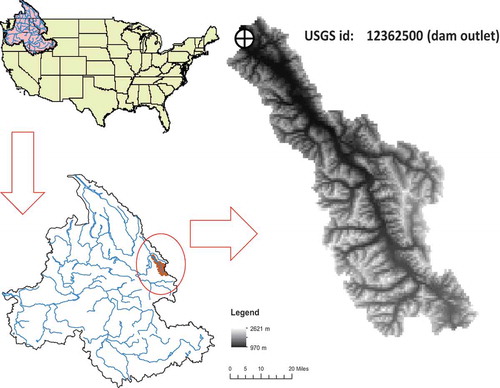
The Hungry Horse Dam was constructed mainly for flood control, irrigation, navigation, streamflow regulation, hydropower generation and recreation (Simons and Rorabaugh 1971). The dam and power plant are operated by the United States Bureau of Reclamation. The dam has a height of 172 m and a storage capacity of about 4.276 km³. The outlet discharge capacity is 397 m³/s at hollow-jet valves and 255 m³/s at the power plant. The installed energy capacity of the dam is 428 000 kW.

2.1 Observed data

In this study, we use daily streamflow data observed in the outlet of the Hungry Horse Dam and the naturalized version of these data. Different institutions, e.g. U.S. Geological Survey, use the publicly available naturalized streamflow series, i.e. NRNI data, provided by the Bonneville Power Administration (http://www.bpa.gov/power/streamflow/default.aspx, accessed 16 February 2015), to calibrate different hydrological models.

The naturalization process has two main components to reverse the effects of irrigation depletion and flow regulation. Unregulated flow estimation is done for every river reach based on mass balance, i.e. gains and losses. A reach gain is then equal to the total of inflow and irrigation-return subtracted from the total of outflow, diversion, evaporation and delta storage change:

(1)

where A/ARF is the ratio of total outflow to average regulated inflows, E/EE is the ratio of site evapotranspiration to accumulated evapotranspiration, and D/DD is the ratio of site irrigation depletion to accumulated depletion. Readers are referred to the previous studies by Naik and Jay (2005) and Acharya and Ryu (2013) for details of streamflow data naturalization (virgin flow calculation) and disaggregation of monthly data to daily data, respectively, in the United States.

In addition to the streamflow data, daily precipitation (P) and potential evapotranspiration (PET) averaged over the basin are analysed. For that, a newly updated gridded daily precipitation (P) dataset (Livneh et al. 2013) is used in this study. The data are available at 6 km (1/16 degree) resolution and comprise observations from the National Climatic Data Center stations (Table 1). Daily PET data are estimated based on daily temperature measurements (Livneh et al. 2013) and National Weather Service monthly PET products (Koren et al. 1998).

Table 1. Overview of observed data used.

Variable	Name	Period	Spatial resolution	Latitude and longitude	Source
Q (daily)	Discharge	1929–2000	Point	Lat: 48.3417 Lon: 114.0083	BPA (HGH5N) and USGS (12362500)
P (daily)	Precipitation	1929–2000	Basin average	–	Livneh et al. (2013)
PET (daily)	Potential evapotranspiration	1929–2000	Basin average	–	Livneh et al. (2013) and Koren et al. (1998)

Precipitation and potential evapotranspiration variables were used due to them being the main climatic drivers for streamflow dynamics, and analysing the effect of climatic variables—e.g. precipitation and potential evapotranspiration—is important in gaining information about the interactions of such processes for the pre- and post-dam periods (Szolgayova et al. 2014). Additionally, naturalized flow series based on NRNI estimations are the result of streamflow and evapotranspiration and an indirect effect of precipitation. Thus, we focus on the streamflow, precipitation and evapotranspiration dataset to understand the potential effects of the dam for different periods. However, the proposed methodology can be applied to any correlated time series to analyse the exchanged relationship within different periods.

3 Methods

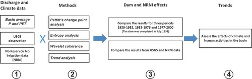
In this study, different statistical methods are applied to detect a possible change in the underlying dynamics resulting from dam construction and the synthetic (naturalized) data are analysed to determine whether the flow dynamics are recovered (Fig. 2). Also, we apply trend analysis to check whether human activities or climatic change, or both, are dominant in trends of P, PET and Q.

Figure 2. Framework for assessing the effects of dam construction and climate in the Hungry Horse River basin.

3.1 Pettitt’s change point analysis

Investigating possible change points in streamflow time series in the Columbia River basin is important for local planning and management of water resources under the pressure of climate change and concentrated anthropogenic effects. Pettitt’s test (1979) has low sensitivity to outliers and has been widely used in different hydrological studies (Li et al. 2014). The test statistic depends on the null hypothesis that there is no statistically meaningful difference between the distributions of two segments that are arbitrarily divided. Let and be sub-series of X_T divided by a change point t₀; then a statistical index U_t,_T can be computed as:

(2)

where

(3)

The possible change point can be found where and the significance level of the test is given by:

(4)

If p < α, the null hypothesis is rejected and x_τ is a significant change point at significance level α.

3.2 Entropy analysis

Entropy is commonly used as an indicator of complexity of dynamical systems. A higher degree of complexity leads to larger entropy values and vice versa. To quantify the complexity, Pincus (1991) proposed approximate entropy, which is efficient in short and noisy data (Zhou et al. 2012). However, since the approximate entropy has a bias in the entropy calculation (Yan et al. 2011), Richman and Moorman (2000) introduced the sample entropy (SampEn), which is a computationally more efficient and straightforward approach, and is less dependent on record length in comparison to the approximate entropy (Zhang et al. 2012c). The SampEn can be calculated based on the following four steps (Richman and Moorman 2000, Yan et al. 2011):

1. The m-dimensional vector can be reconstructed from a scalar time series , as where .

2. where and but denotes the maximum distance between X(i) and X(j).

3. The probability of X(j) within tolerance r of X(i) can be defined as the density in m-dimensional space as , .

4. The average of for all i is where . The densities in m- and m + 1-dimensional spaces, sample entropy, can be calculated from .

Despite the above-mentioned advantages, the time scale selected in the sampling phase can influence the performance of SampEn. Costa et al. (2002) proposed a multi-scale entropy (MSE) analysis to calculate SampEn at multiple time scales. In the MSE analysis, from a simple series , a coarse-grained time series is defined with a scale factor τ () as follows:

(5)

When τ is equal to one, the time series is same as the original series. Finally, SampEn is estimated for all scale factors τ in the coarse-grained time series. In the MSE analysis, m and r are taken as 2 and 0.2σ based on the study by Chou (2012). It should be noted that σ denotes the standard deviation of the original time series.

3.3 Wavelet transform

The wavelet transform is used to detect intermittent periodicities without the stationarity assumption as in Fourier analysis. Covering the possible dominant frequencies, the wavelet transform has been found to be an appropriate tool to analyse geophysical and hydrological time series (Coulibaly 2004). The wavelet transform of a discrete time series X_t, with time step δt (i.e. sampling period) is defined as:

(6)

where

(7)

is defined as a scaled and translated mother wavelet with dilatation parameter s,, and translation parameter u,, the asterisk represents the complex conjugate and N is the length of the time series. While the choice of wavelet depends on the signal type (Zhang et al. 2012a), we employed the Morlet wavelet , where ω₀ (ω₀ = 6 used here) denotes non-dimensional frequency, since it provides a good balance between time and frequency localization (Grinsted et al. 2004). Then the wavelet power spectrum can be denoted as (Torrence and Compo 1998), which gives the variance as a function of scale (period) and time.

To ignore the edge effects we used the cone of influence (COI), which is defined as the e-folding time for wavelet power at each scale. Here, the COI is chosen as the wavelet power has dropped to e⁻², as mentioned in the study by Grinsted et al. (2004). The significance of the wavelet power can be assessed by comparing the theoretical wavelet power spectrum of a red noise model with the obtained wavelet power spectrum. Following the Monte Carlo procedure introduced by Torrence and Compo (1998), the power spectrum is statistically significant if it has greater than 95% confidence for a red noise process with the first autocorrelation calculated from the observed time series. More details about this procedure are explained in Grinsted et al. (2004) and Zhang et al. (2007).

To determine the phase relationship, the mean angles, i.e. a_i (), over regions with statistically significant spectra (>95%) were used (Grinsted et al. 2004). These can be defined as:

(8)

3.4 Cross-wavelet transform (XWT) and wavelet coherence (WTC)

The relationship of two time series at various temporal scales and periods can be estimated by cross-wavelet transform and wavelet coherence by revealing areas of high common power. Introduced by Torrence and Compo (1998), wavelet transforms W_X and W_Y of X and Y time series can be used to obtain the cross-wavelet spectrum W_XY(s, u) as:

(9)

where the asterisk marks complex conjugation. Cross-wavelet power is calculated as , and the phase relationship in time–frequency space between the time series is analysed as an angle of the complex part of the cross-wavelet transform as .

While the cross-wavelet spectrum shows the zones with a common high power, wavelet coherence demonstrates the intensity of the covariance in time–frequency space (Zhang et al. 2007). Similarly to the autocorrelation function, the wavelet coherence is defined as (Torrence and Webster 1999):

(10)

where S is a smoothing operator and can be given by:

(11)

where S_scale and S_time denote filtering along the wavelet scale axis and smoothing in time, respectively. A common smoothing operator for the Morlet wavelet is introduced as (Torrence and Compo 1998):

(12)

(13)

where c₁ and c₂ are constants, and ∏ is the rectangle function. We used 0.6 as the decorrelation length of scale for the Morlet wavelet in Equation (13) based on previous empirical studies (Torrence and Compo 1998). Again, the Monte Carlo statistical significance test is used for cross-wavelet significance.

4 Results and discussion

4.1 Pettitt’s change point analysis

The results of Pettitt’s test show a change point in March 1953 in the USGS streamflow time series when the dam started to operate (Fig. 3). However, March 1950, the possible starting point of the naturalization process, is assigned as a change point in the naturalized streamflows. Therefore, the study period for both streamflows can be divided into two periods, the pre-change (January 1929–December 1952) and post-change (January 1953–December 2000) based on the change points. However, the post-dam period was further divided into two periods each with length equal to that of the pre-dam period, i.e. January 1953–December 1976 and January 1977–December 2000, to keep the effects of data length on the entropy results to a minimum.

Figure 3. Change points of streamflows detected by Pettitt’s test in (a) USGS (b) naturalized time series for 1929–2000.

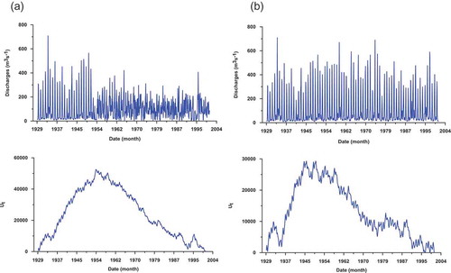
Pettitt’s change point analysis does not provide a reason for the abrupt change in level, and additional analyses should be done to detect abrupt changes in variance (Zhang et al. 2014). Further, as Mallakpour and Villarini (2015) indicated, the chance of detecting abrupt shifts increases as the length of data increases and Pettitt’s change point analysis performs when the magnitude of the shifts is about 5% of the mean of the data before the break. However, the analysis is less sensitive to outliers and has been widely used to detect abrupt changes in hydrological data (e.g. Miao et al. 2012, Guo et al. 2014, Mallakpour and Villarini 2015). Non-parametric Pettitt’s change point analysis is useful when the data considered do not follow a specific distribution, as required for parametric tests, and, as suggested by Villarini et al. (2009), trend analysis should be applied to different segments after employing change point analysis to ensure the validity of the statistical inferences. It is possible statistically to determine the baseline period and segments of time series for detecting the impacts of the dam on streamflow dynamics for different periods.

As noted by Burn et al. (2004), a river’s hydrological trends are associated with changes in both hydro-climatological and large-scale atmospheric progression and sub-segmentation of a streamflow time series is more suitable to study the long-term behaviour of a river (Seyam and Othman 2014), since yearly changes may not be sufficient to portray the long-term changes. Sub-segmentation of data can thus be helpful for analysing long-term changes where sub-segments are formed by consecutive years that show similar hydrological characteristics (Descroix et al. 2012). Similarly, abrupt changes due to dam construction have been found by Seyam and Othman (2014), Guo et al. (2014), Li et al. (2015) and Shi and Wang (2015), where the results have revealed that sub-segmentation is important to better understand the reasons for the abrupt changes and characteristics of the changes in streamflow caused by both natural and anthropogenic factors, such as climate patterns, changes in land use and land cover, and hydraulic structures.

4.2 Entropy analysis

The SampEn and MSE were applied to investigate the changes in the complexity of the USGS (abbreviated as -U in Fig. 4) and NRNI (abbreviated as -N) streamflow time series for the three periods (Q1: 1929–1952, Q2: 1953–1976 and Q3: 1977–2000). For the SampEn, the values of the dimension m and tolerance r are usually taken as 2 and 0.1–0.25σ, respectively (Chou 2012). However, without knowing the underlying dynamics of streamflow, it is hard to find an appropriate value of r (Xie et al. 2010). Therefore, we calculated the SampEn for r varying from 0.1 to 0.25σ in steps of 0.005 for consistency in our results (Fig. 4).

Figure 4. Entropy values of USGS (abbreviated as -U) and NRNI (abbreviated as -N) datasets as a function of tolerance r and scale τ. SampEn is the natural logarithm of the conditional probability of remaining similar at the next point within the tolerance r for which two sequences are similar for m (embedding) consecutive points. While SampEn is calculated by fixing τ = 1, MSE considers also other scales.

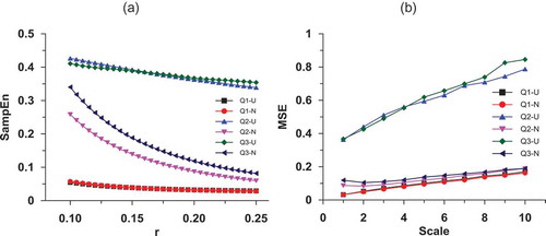
The SampEn seems to be consistent and shows decreases as the tolerance increases (Fig. 4(a)). The entropies show similar behaviour for the streamflow time series from the USGS and NRNI datasets in the pre-dam period; however, the entropies in the post-dam period are different from those estimated for the pre-dam period. We can conclude that the construction of the dam changed the underlying complexity of the river. Additionally, while the USGS flows in the post-dam period (Q2-U and Q3-U) show similar complexities, those of the NRNIs (i.e. Q2-N and Q3-N) show different characteristics in this period. Interestingly, the naturalization process leads to lower complexities (i.e. a higher orderliness) than the USGS flows, and therefore the underlying dynamics/complexities are not recovered by the naturalization process.

Unlike the SampEn, the MSE calculates entropies over multiple temporal scales using a multi-scale structure in the discharge series and provides various entropy values at longer time scales. Figure 4(b) shows that there are large differences between the entropies of USGS and of NRNI data in the post-dam period, of which the former is higher. Here, the naturalization process also lowers the entropy of streamflow. Similar to the SampEn, there are significant differences in the MSE values for the pre-dam and post-dam periods; evidently, the construction of the dam increased the complexity. Further, there is a change in the scaling behaviour of USGS (Fig. 4(b)). The MSE values of Q2-U are close at 1-day and higher than MSE values of Q3-U at other scales. However, when τ > 4 days this relationship is inverted, and the entropies of Q3-U become greater than Q2-U. This could be the reason for changed relationship with an increasing tolerance value between Q2-U and Q3-U (Fig. 4(a)). The reasons for the changes in entropies at τ > 4 days may be changes in land use, land cover (Li and Zhang 2008) and climate. Li and Zhang (2008) proposed that a river system without human intervention should attain its highest entropy, which can be considered as the “healthy system”, and changes in land cover and land use could lower complexities in a river system. However, our results show that higher entropies do not always mean healthier river system and dam construction can distort river complexities and lead to higher entropies.

The most striking result to emerge from Figure 4(b) is that the dam-affected USGS streamflows (Q2-U and Q3-U) show significantly higher entropies than the pre-dam streamflows (Q1-U). Since the entropies estimated from the post-dam NRNI data (Q2-N and Q3-N) are lower than those estimated from the USGS post-dam data (Q2-U and Q3-U), one can say that the naturalized streamflows are more predictable than the USGS observations. This also follows from the fact that hydrological models are mostly designed to simulate natural flow and they do not account for regularized flow in a basin, otherwise the model calibration becomes impractical. The scaling behaviour of NRNI streamflow time series is consistent (Fig. 4(b)). Table 2 shows the descriptive statistics before and after 18 July 1953 when the dam was completed. There was no change of PET before and after the dam. Precipitation characteristics (microclimatology) changed slightly after the dam was built. The median precipitation increased from ~0.7 mm/day to 1.3 mm/day, showing an increase in precipitation falling on the basin. It is apparent from this table that naturalized and USGS streamflow time series show different patterns, especially after completion of the dam. Part of the difference can be explained by the climate-change-related trends and alteration in streamflow. However, the difference in maximum streamflow before and after the dam is still significant, increasing from 1155 m³/s to 1179 m³/s.

Table 2. Basic characteristics of daily flows, precipitation and potential evapotranspiration before and after the construction of the reservoir.

	Min	25th quantile	Median	75th quantile	Max
Before dam – NAT	1	17.3	29.4	99.1	1155.3
After dam – NAT	0.5	23.1	39.1	102.8	1578.7
Before dam – USGS	0.2	16.8	28.3	93.4	1155.3
After dam – USGS	1.6	14.2	69.7	173.9	631.5
Before dam – P	0	0	0.7	3.1	108.9
After dam – P	0	0.1	1.3	5	92.2
Before dam – PET	0.4	0.6	1.6	3.4	4.4
After dam – PET	0.4	0.6	1.6	3.4	4.4

The main reason for applying entropy analyses on the daily scale is that the information obtained from sample entropy decreases from high resolution (i.e. daily scale) to low resolution (i.e. bi-monthly scale), which is inconvenient for comparison of results during different periods. For instance, the results (not shown) indicated that the general behaviour of SampEn as a function of r remains stable up to the bi-monthly scale. However, while SampEn of Q3-U for monthly data is higher than Q2-U at the monthly scale, this relationship is reversed at the bi-monthly scale. Additionally, unstable behaviour for MSE as a function of scale was obtained for monthly and bi-monthly data (not shown), showing that complexity depends on the temporal scale (López-Ruiz et al. 1995). These results are in agreement with the findings of Chou (2014), who found different complexities and predictabilities for various temporal scales with inconsistencies. The main reason for such behaviour of complexity may lie in the number of data points and streamflow patterns resulted from sampling. However, this feature of streamflow time series may be helpful in determining the optimal temporal scale for forecasting purposes, which deserves further investigation.

To check the robustness of the behaviour of SampEn and MSE, results for different lengths (25% and 50% of data points were randomly removed) of streamflow data were obtained (not shown). While consistent behaviour of SampEn and MSE values was seen, the resulting values were different—because of being length dependent (Wu et al. 2016)—from the obtained values for the full-length original series.

Our results are in agreement with Zhou et al. (2012), who found that construction of river dams could significantly increase the degree of complexity of streamflow time series. However, Huang et al. (2011) concluded that the increase in discharge complexity might be due to the rainfall complexity, while flow complexity loss may result from human activities, especially reservoir construction, which leads to more regular time series. Although reservoir construction could lead to more regular series, it is also possible to obtain more irregular series with sharp increases and decreases in river flow in the post-dam period (e.g. outflow processes after power generation), as in the Hungry Horse reservoir and the study by Zhou et al. (2012). Zhang et al. (2012c) found no evidence regarding the effect of the Gezhouba Dam (China) on the complexity of the Yangtze River, and concluded that the considerable flood storage reserves of the lake systems—Poyang and Dongting—enhance long-range correlation and decrease regularity of streamflow, coupled with different rainfall–landform–runoff relationships between the various stations rather than the impact of the dam. As a result, different effects of human activities can lead to a different degree of complexity in a river system in addition to the buffering effects of reservoirs, e.g. diminishing small runoff fluctuations due to water storage. Further, since the inherent complexity of naturalized streamflows is different from those of the original series, the necessity to incorporate an entropy adjustment between the pre- and post-dam periods for NRNI is evident.

Complexity is related to the capability of a river system to adapt to hydrological changes, lower peak flows, and increased flow durations (Li and Zhang 2008). Thus, it is important to determine the complexities of a river at pre- and post-dam periods to reveal whether it becomes more random/unpredictable or more regular due to human activities, for management purposes. Compared with traditional entropy measures, SampEn and MSE are more efficient and suitable for analysing systems that have multiple temporal scale characteristics (Sang 2013). However, while being computationally less demanding and easy to use, the results indicate that estimated SampEn and MSE values are influenced by different temporal scales. SampEn remains stable up to bi-monthly scale while unstable behaviour for MSE as a function of scale was obtained for monthly and bi-monthly datasets. As noted by Wu et al. (2016), as a cornerstone of MSE, the SampEn is length dependent, which leads to erroneous estimations or even undefined entropy values for short time series. Several algorithms have been proposed, such as the refined MSE (Valencia et al. 2009) and the modified MSE for short-term time series (Wu et al. 2013), which are computationally expensive, to overcome this issue. Furthermore, SampEn and MSE cannot be calculated for the variability of rainfall and streamflow jointly. Since the time–space variability of the marginal entropy of streamflow depends on the intensity–duration–frequency of rainfall, Shannon entropy could provide a better framework to study the spatiotemporal variability of rainfall and streamflow and deserves further investigation (Silva et al. 2015).

Finally, due to the inherent sensitivity of SampEn to the choice of the parameter r, validity of regularity or complexity of hydrological time series should be sought in pre-defined ranges of r. However, Li and Zhang (2008), Zhang et al. (2012c) and Chou (2014) used fixed values of r of 0.15σ and 0.2σ. Nevertheless, r must be sufficiently large to avoid noise effects in entropy calculations, and some studies (e.g. Pincus and Goldberger 1994, Richman and Moorman 2000) have shown that 0.1–0.25σ is appropriate (Aktaruzzaman and Sassi 2014). In our study, persistence of entropy behaviour for different r values was obtained; we advise using the same approach for ensuring the validity of the entropy results or employing a surrogate test method coupled with the iterated amplitude-adjusted Fourier transform (IAAFT) (Schreiber and Schmitz 1996), as shown in Tongal and Berndtsson (2016).

4.3 Wavelet cross-spectrum and coherence analysis

Many aspects of a streamflow regime, including periodicity, can be distorted by the construction of a dam, and new cycles can form that are not related to the natural hydrological regime, a possible reason for a change in entropy (White et al. 2005). The wavelet power spectra for the USGS discharge and precipitation are presented in Figure 5. The black line is the COI, where the variance is reduced because of the edge effect. Enclosed regions with solid black contours represent statistically significant power against a red noise process at 95% confidence level. In Figure 5(a), the power for the discharge is distributed with peaks in the 6- and 12-month bands until 1953, and the power for the precipitation (Fig. 5(b)) shows peaks in the 12-month band from 1950 to 1982. It is clear that dam construction distorted the 6–12 month cycle of USGS discharges. While the precipitation has significant wavelet power for 1950–1982, the USGS streamflow has significant wavelet power until 1953, which could be a clue to the changed relationship between these variables. There is no clear link between the cycles of USGS streamflow and precipitation; however, to portray the shared patterns, the cross-wavelet power spectrum (XWT) and wavelet coherence (WTC) between discharge and precipitation are analysed in the following paragraphs.

Figure 5. Wavelet spectra of (a) USGS streamflow and (b) precipitation, (c) cross-wavelet spectrum and (d) wavelet coherence spectrum. Arrows show the phase relationship between the respective time series. Arrows pointing right indicate that the two time series are in-phase, pointing left indicate that they are in opposite-phase, and pointing down indicate that precipitation leads discharge.

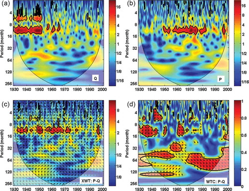
The XWT of USGS streamflow and precipitation is shown in Figure 5(c). It should be noted that the 12-month band from approximately 1932 to 1975 is a significant common power. In this period, a clear change in phase relationship between precipitation and streamflow can be observed after 1953. Until this year, precipitation and discharge have approximately 90° difference, with a lead time of ~3 months; however, in the post-dam period the precipitation and discharge are in a phase relationship until 1975 (Fig. 5(c)). Although the cross-wavelet power shows frequency clusters with common high power, giving a quantity between 0 and 1 and showing significant coherence, indicating the skill of the WTC tool.

The WTC of precipitation and discharge (Fig. 5(d)) shows a relatively large region in the 9–21-month band during 1930–1945 with 90° phase angle. It also shows the in-phase relationship in 1960–1965, and after this period the 9–21-month cycle is lost. However, relatively long cycles in the approximately 4–5-year band during 1935–1955, 2–4-year band during 1955–1965 and 4–11-year band during 1968–1995 are persistent between the streamflow and precipitation. Similarly to Zhang et al. (2007), human activities such as constructing a dam are influential in USGS streamflow for short periods, while precipitation is more influential for long periods. The phase relationship between precipitation and discharge can be seen in Figure 5(d). The phase angle is approximately 90° during 1935–1945 in the 4–5-year band, showing that precipitation leads discharge by 1–1.25 years. Further, precipitation and discharge are in phase during the 1945–1955 period, and precipitation leads discharge by 0.5–1 year during 1955–1965. In the last part, during 1968–1995 precipitation leads discharge by approximately 1–1.5 years. Relatively stable lead times for precipitation are dominant for long cycles whereas distorted lead times are revealed for shorter periods, indicating that construction of the dam has no influence on the relationship between discharge and precipitation in longer cycles. However, the dam affected the relationship in shorter cycles, resulting in a complex precipitation–discharge relationship. Changed lead times can be used for determining optimal lag times for forecasting models, as indicated by Yu et al. (2014), where the authors developed regression models with optimum lag time nodes between different stations along the Yangtze River with the help of the phase relationship obtained.

The naturalization process did not affect the short-term variability of streamflow in the 6- and 12-month bands (Fig. 6(a)). Additionally, the phase relationship between precipitation and streamflow is captured in the post-dam period (Fig. 6(c)) where precipitation leads discharge by 135° (approximately 4.5 months). In the pre-dam period, precipitation leads discharge by 90° (i.e. 3 months). The small change in the lead time could result from the naturalization process.

Figure 6. Wavelet spectra of (a) NRNI streamflow and (b) precipitation, (c) cross-wavelet spectrum and (d) wavelet coherence spectrum. Arrows show the phase relationship between the respective time series. Arrows pointing right indicate that the two time series are in-phase, pointing left indicate anti-phase, and pointing down indicate that precipitation leads discharge.

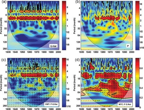
The coherence between precipitation and NRNI streamflow, estimated using the WTC analysis, is more pronounced than the coherence between precipitation and USGS streamflow. Precipitation is one of the main driving factors in obtaining NRNI streamflows. Relatively more stable lead times in longer cycles, e.g. the 4–5-year band of USGS and NRNI streamflows, indicate that short-term precipitation should be explicitly considered in a naturalization framework. The naturalization process added artificial coherence to the 9–21-month band in the post-dam period and to the 2–3.5-year band after the year 1965: a possible reason for lower complexity in the NRNI data as compared to the USGS data. Further, the NRNI data show better coherence between precipitation and streamflow than the USGS data. To distinguish between human activities and climatic changes, we applied the Mann-Kendall trend test on P, PET and Q series. We found weak positive trends in all three variables, indicating that the effect of human activities (e.g. dam construction) on the alteration of flow magnitude and dynamics can overlap with the effect of climatic changes in the basin.

Efficient reservoir management and control provide efficient reservoir yields and better flood control. The main impact of reservoir construction is to change the seasonal distribution of available water, reducing peak flows in the flood season and weakening the natural variability of the water discharge (Liu et al. 2012). Moreover, Zhang et al. (2007) concluded that human activities, such as constructing a dam, are influential on streamflow over short periods while precipitation is more influential for long periods. Thus, monthly scale analysis provides efficient resolution since it reveals high-frequency patterns—infra-annual/seasonal—(Coulibaly 2004) for studying the long-term behaviour of streamflow, precipitation and evapotranspiration, similar to the studies of Labat et al. (2005), Melesse et al. (2011), Niu (2013), Wang et al. (2013a) and Zhang et al. (2012b). Furthermore, the wavelet results on weekly and bi-monthly data for streamflow and precipitation indicate that (not shown) the same phase relationships as for monthly data are obtained for similar years, while the frequencies for the bi-monthly data are divided by two (e.g. the periodicities at the yearly scale for monthly data are now seen for the half-year period for bi-monthly data) and the frequencies for the weekly data are increased (e.g. the yearly dominant frequency is seen at about 52 weeks for USGS flow). Finally, Pettitt’s change point analysis also indicates the same date as a change point; thus, based on these results we can verify the validity of the results. However, since the monthly scale was considered, it is important to have sufficiently long series of records to reveal the impact of the dam, which is an important boundary effect on the wavelet analysis of damming effects, where long-term and quality data may not always be available. Also, it should be noted that the wavelet analyses employed are not suitable for time series having unequal lengths and covering different time intervals (Briciu and Mihăilă 2014).

While wavelets have been employed in several hydrological time series analyses including streamflow forecasting (Kisi 2010, Badrzadeh et al. 2013), drought forecasting (Belayneh et al. 2014), modelling rainfall–runoff relationships (Labat et al. 1999), forecasting of groundwater level (Adamowski & Chan, 2011) and water quality (Wang et al. 2013b), and analysing the impacts of climatic oscillations on river flows (Zhang et al. 2007, Labat 2010, Briciu and Mihăilă 2014), there are limited applications (White et al. 2005, Yu et al. 2014, Zhao et al. 2014) showing the impacts of dams on hydrological changes. Some drawbacks have been reported for widely employed methods for determining the impact of dams on streamflow dynamics, such as indicators of hydrological alteration (e.g. Chen et al. 2015, Wang et al. 2015, Duan et al. 2016) and flood frequency analysis (Maingi and Marsh 2002, Li et al. 2015, Ghosh and Guchhait 2016). Application of indicators of hydrological alteration is time consuming and requires daily flow data, which are not readily available in all regions. Furthermore, based on a priori assignment of the time intervals, the analysis may fail to evaluate changes in cyclic phenomena and therefore changes in river flow dynamics should be known beforehand. This is important where a poor quality record of operation could make the determination of the timing of events—e.g. change in management (White et al. 2005)—more difficult. As indicated by Maingi and Marsh (2002), flood frequency analysis is based on the annual maximum series and, thus, insignificantly small floods or massive floods can be included or excluded, respectively. Also, floods with a recurrence interval of less than 1 year cannot be determined at the annual scale. However, wavelet analyses are promising tools to improve these shortcomings by allowing recognition of the changes in cyclic phenomena occurring at any time and scale (White et al. 2005).

The SampEn and MSE are less efficient in non-stationary time series and cannot describe the reason for changing entropy values among different periods. We hypothesize that a changed underlying cross-correlation between streamflow and precipitation due to dam construction could lead to such a result. Moreover, an analysis of how the scale contents of streamflow and precipitation change over different periods is crucial for complicated hydrological processes (Labat, 2005). Since the traditional cross-correlation analysis methods can only be used to analyse the time series with linear and ergodic properties and do not describe the cross-correlations under certain temporal scales (Sang 2013), wavelet cross-correlation analyses—XWT and WTC—are suitable methods for this purpose. Also, the Fourier transform is designed for stationary signals consisting of linear, independent and non-changing periodicities over time (Labat 2005), whereas it is not well suited for the time-dependent scaling behaviour of streamflow and precipitation. The wavelet transform, however, is very efficient for tracking the time-scale evolution with multi-resolution analysis of hydrological time series that are highly non-stationary and operating under a broad range of scales (Pandey et al. 1998). Additionally, one advantage of the wavelet transform over the Fourier transform is that the former is scale dependent, and it does not require a pre-determined scale which would limit the frequency range (Coulibaly 2004). However, since both wavelet and decomposition level choice is subjective, more objective and robust methods are needed (Sang 2013). Also, as noted by Chen and Xie (2007), a small shift in the input series would lead to very different output wavelet coefficients, which is one of the main problems of the conventional wavelet transform based on a real-valued wavelet function and scaling function.

5 Conclusions

USGS streamflow observations recorded at the outlet of the Hungry Horse Dam were compared with the synthetic times series estimated based on the no-regulation and no-irrigation (NRNI) assumption. The comparison was done for three periods, one pre-dam and two post-dam, using different methods i.e. change point, entropy and wavelet analyses. Trends in precipitation, potential evapotranspiration and streamflow series were also compared to comprehend the effects of dam and climatic changes.

Pettit’s change point analysis showed that dam construction caused a change point in the monthly time series in both USGS and NRNI data. Based on the results of entropy analysis, the dam changed the underlying complexities of the river, and the naturalization process was not able to recover them completely. This is an important finding, as the NRNI streamflow series are often used in calibration and evaluation of various distributed hydrological models across the USA. The naturalization process should be further investigated since there can be other inevitable uncertainties due to seasonality and cyclic events. Wavelet analysis results were found to be instrumentally useful to confirm the change in phase relationship between precipitation and streamflow after the dam construction. The framework applied in this study can be generalized to any other river in the world to reveal the effects of a dam on linear and nonlinear streamflow dynamics. This paper focused on the differences in streamflow quantity over different periods. However, further work should examine the effects of a dam on water quality, eco-hydrology and microclimatology of the domain using different variables such as soil moisture and the frequency of rainy days.

Acknowledgements

The NRNI data were provided by the Bonneville Power Administration (available at http://www.bpa.gov/power/streamflow/default.aspx), and accessed in February 2015. The naturalization methodology was provided by Bob Lounsbury from the U.S. Bureau of Reclamation. The codes for wavelet analyses can be accessed at http://noc.ac.uk/using-science/crosswavelet-wavelet-coherence. We acknowledge financial support for the SPACE project (http://www.space.geus.dk/) by the Villum Foundation (http://villumfonden.dk/) through their Young Investigator Programme (grant VKR023443).

Disclosure statement

No potential conflict of interest was reported by the authors.

Additional information

Funding

This work was supported by the Villum Foundation (grant VKR023443).

References

- Acharya, A. and Ryu, J., 2013. Simple method for streamflow disaggregation. Journal of Hydrologic Engineering, 19 (3), 509–519. American Society of Civil Engineers doi:10.1061/(ASCE)HE.1943-5584.0000818
- Adamowski, J. and Chan, H., 2011. A wavelet neural network conjunction model for groundwater level forecasting. Journal of Hydrology, 407, 28–40. Available from http://www.sciencedirect.com/science/article/pii/S0022169411004100
- Aktaruzzaman, M. and Sassi, R., 2014. Parametric estimation of sample entropy in heart rate variability analysis. Biomedical Signal Processing and Control, 14, 141–147. Available from http://www.sciencedirect.com/science/article/pii/S1746809414001177
- Badrzadeh, H., Sarukkalige, R., and Jayawardena, A.W., 2013. Impact of multi-resolution analysis of artificial intelligence models inputs on multi-step ahead river flow forecasting. Journal of Hydrology, 507, 75–85. Elsevier B.V. doi:10.1016/j.jhydrol.2013.10.017
- Belayneh, A., et al., 2014. Long-term SPI drought forecasting in the Awash River Basin in Ethiopia using wavelet neural network and wavelet support vector regression models. Journal of Hydrology, 508, 418–429. Available from http://www.sciencedirect.com/science/article/pii/S0022169413007968
- Briciu, A.-E. and Mihăilă, D., 2014. Wavelet analysis of some rivers in SE Europe and selected climate indices. Environmental Monitoring and Assessment, 186, 6263–6286. doi:10.1007/s10661-014-3853-z
- Burn, D., Cunderlik, J., and Pietroniro, A., 2004. Hydrological trends and variability in the Liard River basin/Tendances hydrologiques et variabilité dans le basin de la rivière Liard. Hydrological Sciences Journal, 49, 53–67. doi:10.1623/hysj.49.1.53.53994
- Chen, G. and Xie, W., 2007. Pattern recognition with SVM and dual-tree complex wavelets. Image and Vision Computing, 25, 960–966. Available from http://www.sciencedirect.com/science/article/pii/S0262885606002198
- Chen, Q., et al., 2015. Downstream effects of a hydropeaking dam on ecohydrological conditions at subdaily to monthly time scales. Ecological Engineering, 77, 40–50. doi:10.1016/j.ecoleng.2014.12.017
- Chou, C.-M., 2012. Applying multiscale entropy to the complexity analysis of rainfall-runoff relationships. Entropy, 14 (12), 945–957. doi:10.3390/e14050945
- Chou, C.-M., 2014. Complexity analysis of rainfall and runoff time series based on sample entropy in different temporal scales. Stochastic Environmental Research and Risk Assessment, 28 (6), 1401–1408. doi:10.1007/s00477-014-0859-6
- Costa, M., Goldberger, A.L., and Peng, C.-K., 2002. Multiscale entropy analysis of complex physiologic time series. Physical Review Letters, 89 (6), 68102. doi:10.1103/PhysRevLett.89.068102
- Coulibaly, P., 2004. Wavelet analysis of variability in annual Canadian streamflows. Water Resources Research, 40 (3), 1–14. doi:10.1029/2003WR002667
- Descroix, L., et al., 2012. Change in Sahelian Rivers hydrograph: the case of recent red floods of the Niger River in the Niamey region. Global and Planetary Change, 98-99, 18–30. Availablefrom http://www.sciencedirect.com/science/article/pii/S092181811200149X
- Duan, W., et al., 2016. Impact of cascaded reservoirs group on flow regime in the middle and lower reaches of the Yangtze River. Water, 8 (6). MDPI AG. doi:10.3390/w8060218
- Ghosh, S. and Guchhait, S.K., 2016. Dam-induced changes in flood hydrology and flood frequency of tropical river: a study in Damodar River of West Bengal, India. Arabian Journal of Geosciences, 9 (2), 90. Springer Berlin Heidelberg doi:10.1007/s12517-015-2046-6
- Grinsted, A., Moore, J.C., and Jevrejeva, S., 2004. Application of the cross wavelet transform and wavelet coherence to geophysical time series. Nonlinear Processes in Geophysics, 11 (5/6), 561–566. doi:10.5194/npg-11-561-2004
- Guo, Y., et al., 2014. Quantitative assessment of the impact of climate variability and human activities on runoff changes for the upper reaches of Weihe River. Stochastic Environmental Research and Risk Assessment, 28 (2), 333–346. Springer Berlin Heidelberg doi:10.1007/s00477-013-0752-8
- Hernández-Henríquez, M.A., Mlynowski, T.J., and Déry, S.J., 2010. Reconstructing the Natural Streamflow of a regulated River: a case study of La Grande Rivière, Québec, Canada. Canada Water Resources Journal, 35 (3), 301–316. doi:10.4296/cwrj3503301
- Huang, F., et al., 2011. Flow-complexity analysis of the upper reaches of the Yangtze River, China. Journal of Hydrologic Engineering, 16 (11), 914–919. American Society of Civil Engineers doi:10.1061/(ASCE)HE.1943-5584.0000392
- Kisi, O., 2010. Wavelet regression model for short-term streamflow forecasting. Journal of Hydrology, 389 (3–4), 344–353. Elsevier B.V. doi:10.1016/j.jhydrol.2010.06.013
- Koren, V., et al., 1998. PET Upgrades to NWSRFS, Project Plan. Washington, DC, unpublished report.
- Labat, D., 2005. Recent advances in wavelet analyses: Part 1. A review of concepts. Journal of Hydrology, 314 (1–4), 275–288.
- Labat, D., 2010. Cross wavelet analyses of annual continental freshwater discharge and selected climate indices. Journal of Hydrology, 385 (1–4), 269–278. doi:10.1016/j.jhydrol.2010.02.029
- Labat, D., Ababou, R., and Mangin, A., 1999. Wavelet analysis in karstic hydrology. 2nd part: rainfall-runoff cross-wavelet analysis. Comptes Rendus de l’. Available from http://www.ingentaconnect.com/content/els/12518050/1999/00000329/00000012/art88501
- Labat, D., Ronchail, J., and Guyot, J.L., 2005. Recent advances in wavelet analyses: Part 2—Amazon, Parana, Orinoco and Congo discharges time scale variability. Journal of Hydrology, 314 (1), 289–311. doi:10.1016/j.jhydrol.2005.04.004
- Li, D., Xie, H., and Xiong, L., 2014. Temporal change analysis based on data characteristics and nonparametric test. Water Resources Management, 28 (1), 227–240. Springer Netherlands doi:10.1007/s11269-013-0481-2
- Li, J., Liu, X., and Chen, F., 2015. Evaluation of nonstationarity in annual maximum flood series and the associations with large-scale climate patterns and human activities. Water Resources Management, 29 (5), 1653–1668. Springer Netherlands doi:10.1007/s11269-014-0900-z
- Li, Z. and Zhang, Y.-K., 2008. Multi-scale entropy analysis of Mississippi River flow. Stochastic Environmental Research and Risk Assessment, 22 (4), 507–512. doi:10.1007/s00477-007-0161-y
- Liu, F., et al., 2012. Spatial and temporal variability of water discharge in the Yellow River Basin over the past 60 years. Journal of Geographical Sciences, 22 (2010), 1013–1033. doi:10.1007/s11442-012-0980-8
- Livneh, B., et al., 2013. A long-term hydrologically based data set of land surface fluxes and states for the conterminous United States: updates and extensions. Journal of Climate, 26, 9384–9392. doi:10.1175/JCLI-D-12-00508.1
- López-Ruiz, R., Mancini, H.L., and Calbet, X., 1995. A statistical measure of complexity. Physics Letters A, 209 (5–6), 321–326. North-Holland doi:10.1016/0375-9601(95)00867-5
- Lu, X.X., et al., 2014. Observed changes in the water flow at Chiang Saen in the lower Mekong: impacts of Chinese dams? Quaternary International, 336, 145–157. doi:10.1016/j.quaint.2014.02.006
- Magilligan, F.J. and Nislow, K.H., 2005. Changes in hydrologic regime by dams. Geomorphology, 71 (1–2), 61–78. doi:10.1016/j.geomorph.2004.08.017
- Maingi, J.K. and Marsh, S.E., 2002. Quantifying hydrologic impacts following dam construction along the Tana River, Kenya. Journal of Arid Environments, 50 (1), 53–79. doi:10.1006/jare.2000.0860
- Mallakpour, I. and Villarini, G., 2015. A simulation study to examine the sensitivity of the Pettitt test to detect abrupt changes in mean. Hydrological Sciences Journal. Taylor & Francis. doi:10.1080/02626667.2015.1008482
- Melesse, A.M., et al., 2011. Suspended sediment load prediction of river systems: an artificial neural network approach. Agricultural Water Management, 98 (5), 855–866. doi:10.1016/j.agwat.2010.12.012
- Miao, C.Y., et al., 2012. Spatio-temporal variability of streamflow in the Yellow River: possible causes and implications. Hydrological Sciences Journal, 57 (February 2015), 1355–1367. doi:10.1080/02626667.2012.718077
- Muhlfeld, C.C., et al., 2012. Assessing the impacts of river regulation on native bull trout (salvelinus confluentus) and westslope cutthroat trout (oncorhynchus clarkii lewisi) habitats in the upper flathead river, Montana, USA. River Research and Applications, 28, 940–959. doi:10.1002/rra.1494
- Naik, P.K. and Jay, D.A., 2005. Estimation of Columbia River virgin flow: 1879 to 1928. Hydrological Processes, 19 (9), 1807–1824. doi:10.1002/hyp.5636
- Niu, J., 2013. Precipitation in the Pearl River basin, South China: scaling, regional patterns, and influence of large-scale climate anomalies. Stochastic Environmental Research and Risk Assessment, 27, 1253–1268. doi:10.1007/s00477-012-0661-2
- Pandey, G., Lovejoy, S., and Schertzer, D., 1998. Multifractal analysis of daily river flows including extremes for basins of five to two million square kilometres, one day to 75 years. Journal of Hydrology, 208, 62–81. Available from http://www.sciencedirect.com/science/article/pii/S0022169498001486
- Pettitt, A.N., 1979. A non-parametric approach to the change-point problem. Journal of the Royal Statistical Society. Series C (Applied Statistics), 28 (2), 126–135. Wiley for the Royal Statistical Society doi:10.2307/2346729
- Pincus, S. and Goldberger, A., 1994. Physiological time-series analysis: what does regularity quantify? American Journal of Physiology. Available from http://ajpheart.physiology.org/content/266/4/H1643.short
- Pincus, S.M., 1991. Approximate entropy as a measure of system complexity. Proceedings of the National Academy of Sciences, 88 (6), 2297–2301. doi:10.1073/pnas.88.6.2297
- Poff, N.L., et al., 2007. Homogenization of regional river dynamics by dams and global biodiversity implications. Proceedings of the National Academy of Sciences, 104 (14), 5732–5737. doi:10.1073/pnas.0609812104
- Richman, J.S. and Moorman, J.R., 2000. Physiological time-series analysis using approximate entropy and sample entropy. American Journal of Physiology. Heart and Circulatory Physiology, 278 (6), H2039–H2049. Available from http://ajpheart.physiology.org/content/278/6/H2039.short
- Richter, B.D., et al., 1996. A method for assessing hydrologic alteration within ecosystems. Conservation Biology, 10 (4), 1163–1174. doi:10.1046/j.1523-1739.1996.10041163.x
- Sang, Y.-F., 2013. A review on the applications of wavelet transform in hydrology time series analysis. Atmospheric Research, 122, 8–15. doi:10.1016/j.atmosres.2012.11.003
- Schreiber, T. and Schmitz, A., 1996. Improved surrogate data for nonlinearity tests. Physical Review Letters, 77 (4), 635–638. American Physical Society. doi:10.1103/PhysRevLett.77.635
- Sen, K.A., 2009. Complexity analysis of riverflow time series. Stochastic Environmental Research and Risk Assessment, 23 (3), 361–366. Springer-Verlag doi:10.1007/s00477-008-0222-x
- Seyam, M. and Othman, F., 2014. Long-term variation analysis of a tropical river’s annual streamflow regime over a 50-year period. Theoretical and Applied Climatology, 1–15. Springer Vienna. doi:10.1007/s00704-014-1225-9
- Shi, H. and Wang, G., 2015. Impacts of climate change and hydraulic structures on runoff and sediment discharge in the middle Yellow River. Hydrological Processes, 29 (14), 3236–3246. doi:10.1002/hyp.10439
- Silva, V.D.P.R.D., et al., 2015. Entropy theory for analyzing water resources in northeastern region of Brazil. Hydrological Sciences Journal, Taylor & Francis. doi:10.1080/02626667.2015.1099789
- Simons, W. and Rorabaugh, M. (1971) Hydrology of Hungry Horse reservoir, Northwestern Montana. US Government Printing Office. Available from http://pubs.usgs.gov/pp/0682/report.pdf
- Szolgayova, E., et al., 2014. Long term variability of the Danube River flow and its relation to precipitation and air temperature. Journal of Hydrology, 519, 871–880. Elsevier B.V. doi:10.1016/j.jhydrol.2014.07.047
- Tongal, H. and Berndtsson, R., 2016. Impact of complexity on daily and multi-step forecasting of streamflow with chaotic, stochastic, and black-box models. Stochastic Environmental Research and Risk Assessment. doi:10.1007/s00477-016-1236-4
- Torrence, C. and Compo, G.P., 1998. A practical guide to wavelet analysis. Bulletin of the American Meteorological Society, 79 (1), 61–78. doi:10.1175/1520-0477(1998)079<0061:APGTWA>2.0.CO;2
- Torrence, C. and Webster, P.J., 1999. Interdecadal changes in the ENSO-monsoon system. Journal of Climate, 12 (8), 2679–2690. doi:10.1175/1520-0442(1999)012<2679:ICITEM>2.0.CO;2
- Valencia, J., Porta, A., and Vallverdú, M., 2009. Refined multiscale entropy: application to 24-h holter recordings of heart period variability in healthy and aortic stenosis subjects. IEEE Transactions. Available from http://ieeexplore.ieee.org/xpls/abs_all.jsp?arnumber=4956991
- Villarini, G., et al., 2009. On the stationarity of annual flood peaks in the continental United States during the 20th century. Water Resources Research, 45 (8), n/a–n/a. doi:10.1029/2008WR007645
- Wang, W., et al., 2013a. Characterizing the changing behaviours of precipitation concentration in the Yangtze River Basin, China. Hydrological Processes, 27 (24), 3375–3393. doi:10.1002/hyp.9430
- Wang, Y., Wang, D., and Wu, J., 2015. Assessing the impact of Danjiangkou reservoir on ecohydrological conditions in Hanjiang river, China. Ecological Engineering, 81, 41–52. doi:10.1016/j.ecoleng.2015.04.006
- Wang, Y., et al., 2013b. Monthly water quality forecasting and uncertainty assessment via bootstrapped wavelet neural networks under missing data for Harbin, China. Environmental Science and Pollution Research, 20, 8909–8923. doi:10.1007/s11356-013-1874-8
- White, M.A., Schmidt, J.C., and Topping, D.J., 2005. Application of wavelet analysis for monitoring the hydrologic effects of dam operation: Glen canyon dam and the Colorado River at lees ferry, Arizona. River Research and Applications, 21 (July 2004), 551–565. doi:10.1002/rra.827
- Wu, S., et al., 2013. Modified multiscale entropy for short-term time series analysis. Physica A: Statistical Mechanics and Its, 392, 5865–5873. Available from http://www.sciencedirect.com/science/article/pii/S0378437113007061
- Wu, S.-D., Wu, C.-W., and Humeau-Heurtier, A., 2016. Refined scale-dependent permutation entropy to analyze systems complexity. Physica A: Statistical Mechanics and its Applications, 450, 454–461. doi:10.1016/j.physa.2016.01.044
- Xie, H.-B., Guo, J.-Y., and Zheng, Y.-P., 2010. Using the modified sample entropy to detect determinism. Physics Letters A, 374 (38), 3926–3931. Elsevier B.V. doi:10.1016/j.physleta.2010.07.058
- Yan, K., Huanjie, C., and Songbai, S., 2011. A measure of hydrological system complexity based on sample entropy. Water Resource and Environmental Protection (ISWREP), 2011 International Symposium on, 1, 470–473. IEEE.
- Yang, T., et al., 2008. A spatial assessment of hydrologic alteration caused by dam construction in the middle and lower Yellow River, China. Hydrological Processes, 22 (18), 3829–3843. doi:10.1002/hyp.6993
- Yu, S., Yang, J., and Liu, G., 2014. Impact assessment of Three Gorges Dam’s impoundment on river dynamics in the north branch of Yangtze River estuary, China. Environmental Earth Sciences, 72, 499–509. doi:10.1007/s12665-013-2971-1
- Zhang, J., Li, G., and Liang, S., 2012a. The response of river discharge to climate fluctuations in the source region of the Yellow River. Environmental Earth Sciences, 66 (5), 1505–1512. doi:10.1007/s12665-011-1390-4
- Zhang, Q., et al., 2014. Stationarity of annual flood peaks during 1951–2010 in the Pearl River basin, China. Journal of Hydrology, 519, 3263–3274. Elsevier B.V. doi:10.1016/j.jhydrol.2014.10.028
- Zhang, Q., et al., 2012b. Trend, periodicity and abrupt change in streamflow of the East River, the Pearl River basin. Hydrological Processes, n/a–n/a. doi:10.1002/hyp.9576
- Zhang, Q., et al., 2007. Possible influence of ENSO on annual maximum streamflow of the Yangtze River, China. Journal of Hydrology, 333, 265–274. doi:10.1016/j.jhydrol.2006.08.010
- Zhang, Q., et al., 2012c. The influence of dam and lakes on the Yangtze River streamflow: long-range correlation and complexity analyses. Hydrological Processes, 26 (3), 436–444. doi:10.1002/hyp.8148
- Zhao, G., et al., 2014. Quantifying the impact of climate variability and human activities on streamflow in the middle reaches of the Yellow River basin, China. Journal of Hydrology, 519, 387–398. Elsevier B.V. doi:10.1016/j.jhydrol.2014.07.014
- Zhao, Q., et al., 2012. The effects of dam construction and precipitation variability on hydrologic alteration in the Lancang River Basin of southwest China. Stochastic Environmental Research and Risk Assessment, 26 (7), 993–1011. doi:10.1007/s00477-012-0583-z
- Zhou, Y., et al., 2012. Hydrological effects of water reservoirs on hydrological processes in the East River (China) basin: complexity evaluations based on the multi-scale entropy analysis. Hydrological Processes, 26 (January), 3253–3262. doi:10.1002/hyp.8406