Space–time forecasting of groundwater level using a hybrid soft computing model

ABSTRACT

Forecasting of space–time groundwater level is important for sparsely monitored regions. Time series analysis using soft computing tools is powerful in temporal data analysis. Classical geostatistical methods provide the best estimates of spatial data. In the present work a hybrid framework for space–time groundwater level forecasting is proposed by combining a soft computing tool and a geostatistical model. Three time series forecasting models: artificial neural network, least square support vector machine and genetic programming (GP), are individually combined with the geostatistical ordinary kriging model. The experimental variogram thus obtained fits a linear combination of a nugget effect model and a power model. The efficacy of the space–time models was decided on both visual interpretation (spatial maps) and calculated error statistics. It was found that the GP–kriging space–time model gave the most satisfactory results in terms of average absolute relative error, root mean square error, normalized mean bias error and normalized root mean square error.

KEYWORDS:

• Space–time forecasting
• groundwater level
• artificial neural network (ANN)
• least square support vector machine (LS-SVM)
• genetic programming (GP)
• kriging

Editor D. Koutsoyiannis; Associate editor A. Fiori

1 Introduction

Groundwater level forecasting is one of the most important practices in subsurface hydrological studies. Both spatial and temporal forecasting of groundwater level have attracted equal attention from the research community in the recent past. The models used in subsurface water level prediction have ranged from black box models (e.g. artificial neural networks (ANN) and other models based on artificial intelligence) to white and grey box models (mathematical and conceptual models). However, it is worth mentioning that most of the enormous number of studies done with all these models analysed either the spatial aspect of groundwater level variation or the temporal variation of groundwater level. Studies on the space–time variation of groundwater level are few (Nourani et al. 2008, Tapoglou et al. 2014, Jha and Sahoo 2015). Moreover, sparsity of spatial and temporal data poses major challenges in forecasting. In the present study an attempt has been made to analyse space–time variability and predict one-month advance groundwater levels for a sparsely monitored region with the help of hybrid models.

Hybrid models are generally combinations of classical models and soft computing techniques. Geostatistical kriging is regarded as the most powerful stochastic spatial interpolation technique (Varouchakis and Hristopulos 2013a, 2013b). However, applications to space–time prediction of groundwater levels using kriging techniques have remained very few. A major advantage of kriging is that it is more flexible than other interpolation techniques (Kitanidis 1997). In the spatial estimation of groundwater level, kriging and all its variants (ordinary kriging, universal kriging, co-kriging, kriging with Delaunay triangulation) have been used successfully across the globe (Ahmadi and Sedghamiz 2007, Nourani et al. 2008, Kholghi and Hosseini 2009, Ta’any et al. 2009, Chung and Rogers 2012, Machiwal et al. 2012, Varouchakis and Hristopulos 2013a, 2013b, Tapoglou et al. 2014, Bhat et al. 2015). These geostatistical models were able to simulate spatial groundwater level. For space–time prediction, kriging has been used in conjunction with neural networks to develop neural-geostatistics (Nourani et al. 2008) to model space–time groundwater level.

The ability of ANNs to identify relationships from given patterns has made them useful in solving complex hydrological problems. However, ANNs have not found significant application in spatial modelling. In the present study, the ANN was focused on the temporal aspect of the spatio-temporal model. Several researchers have used ANN for groundwater level prediction using different input parameters (Daliakopoulos et al. 2005, Lallahem et al. 2005, Nayak et al. 2006, Dash et al. 2010, Trichakis et al. 2011, Shiri et al. 2013, Jha and Sahoo 2015). The major limitation of most of the previously developed ANN models is the requirement for a large quantity of data to achieve good training. The models developed in the present study try to overcome this constraint by using a small dataset.

The least square support vector machine (LS-SVM) is a simplified form of SVM that uses equality constraints and adopts the least square linear system as its loss function, which is computationally attractive (Samsudin et al. 2011). The LS-SVM has found successful application in surface hydrology. This method had been used in the recent past as a powerful, nonlinear, black-box regression method for time series analysis (Hwang et al. 2012), flow prediction at daily scale (Bhagwat and Maity 2012) and streamflow forecasting (Shabri and Suhartono 2012). The use of LS-SVM in space–time groundwater level forecasting has never been attempted.

Genetic programming (GP) is an evolutionary algorithm similar to the genetic algorithm and it uses the concept of natural selection and genetics in evolutionary computation (Sreekanth and Datta 2010). Genetic programming has been used in hydrological studies for developing prediction models for rainfall–runoff and river stage forecasting (Sheta and Mahmoud 2001, Babovic and Keijzer 2002, Wang et al. 2009). To date, only one study on groundwater level prediction using GP (Fallah-Mehdipour et al. 2013) has been reported. However, GP has never been used for space–time modelling of groundwater level.

A recent study by Tapoglou et al. (2014) combined ANN and kriging to stimulate spatial and temporal distributions. The ANN models developed by this study, however, used a number of hydro-meteorological data (rainfall, temperature and surface water level measurements). Information on such hydro-meteorological parameters may or may not be available for all places. The models thus developed have limited application. The present study uses only groundwater level data to develop all the models. Hence, the models overcome the limitations of the previously available models. The present work also compares the hybrid models developed using kriging in conjunction with the ANN, LS-SVM and GP models. The use of the LS-SVM and GP models for the space–time study of groundwater level has never been compared. The groundwater level predicted by the temporal models has been fed into the spatial model to give the desired space–time prediction. The present study attempts to find the best model for space–time forecasting of groundwater level in the study area.

2 Study area description

The area selected for the present study is Kanpur city (Fig. 1). It lies between 26°20ʹ38″N and 26°30ʹ49″N latitude and 80°12ʹ50″E and 80°27ʹ28″E longitude, covering an area of 258 km². The city is bounded in the east by the River Ganga and in the west by the River Pandu. Northern and southern boundaries are of a political nature (Dhar 2013, Dhar et al. 2015). Sources of surface water in the city are the River Ganga and the River Pandu catchments. Kanpur is an industrial city with textile, leather, jute and chemical industries. Rapid industrialization and the consequent increase in population have increased the demand for water. The water demand for Kanpur city is approximately 6 × 10⁵ m³/d. However, only 3.85 × 10⁵ m³/d is being supplied to users. The total water supply from treatment plants is about 2.55 × 10⁵ m³/d. Thus, 1.3 × 10⁵ m³/d water is drawn from the subsurface zone (8 × 10⁴ m³/d from 135 tube wells and 5 × 10⁴ m³/d from 9830 hand pumps) (JNNURM 2006). This shortage is resulting in continuous depletion of the water table, presently at the rate of about 45 cm/year throughout the city (Personal communication with State Groundwater Department, Uttar Pradesh).

3 Materials and methods

3.1 Data analysis

The datasets were pre-processed before being used for modelling purposes. The procedures involved in pre-processing of data are explained in the following sections. The datasets were then divided into two sets: a calibration dataset and a testing dataset. Of the 56 well sites, the monthly groundwater level data for 35 sites were used for calibration purpose. Datasets for five sites were selected as testing datasets and the remaining 16 sites were discarded due to partial availability of data. All temporal models were calibrated with the groundwater level data from March 2006 to December 2010. The data from January to June 2011 were used for testing the models. In the spatial models, well sites 3, 24, 32, 35 and 56 were selected for testing the model. All the other sites (1, 5, 6, 7, 8, 9, 10, 11, 13, 14, 15, 16, 17, 20, 21, 22, 23, 25, 28, 29, 33, 34, 36, 38, 39, 40, 43, 44, 45, 49, 50, 51, 52, 54 and 55) were used for calibrating the spatial model. The locations of all the testing and calibration sites for spatial and temporal models are shown in Figure 2(a) and (b). The results obtained from the models were again input to post-processing so as to get results in their original form.

Figure 1. Map of study area showing locations of wells.

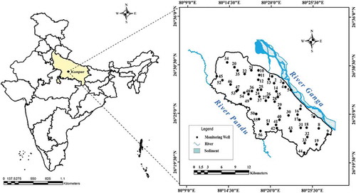
Figure 2. Locations of calibration, testing and discarded sites used for (a) spatial models and (b) temporal models.

3.2 Data processing for temporal models

3.2.1 Pre-processing

Standardization of data was done by subtracting the mean and dividing by the standard deviation. The dataset was thus made to have a mean of 0 and variance of 1 (Wang et al. 2006). This process is also termed deseasonalization. It is done to remove cyclicity or periodicity present in data.

The data were rescaled to values lying in the interval [−1, 1]. This interval was chosen due to the tan-sigmoid transfer function (discussed later in the paper). The tan-sigmoid transfer function is bounded in nature. For rescaling of data, the following formula was used:

(1)

3.2.2 Post-processing

The model outputs were reversely transformed to obtain the results in the original form. For post-processing of data, seasonalization of the data was performed. This is the reverse process to standardization. It is done to bring back the cyclicity or periodicity in the pre-processed data. Rescaled results were scaled back to the original form to get the final results.

3.3 Temporal models used in the study

3.3.1 Artificial neural networks

An ANN discovers the relationship between a set of inputs and desired outputs without giving any information about the actual processes involved (Haykin 1994)). For the present study, a single hidden layer feedforward was used for time series modelling and forecasting of groundwater level. In the present ANN model, seven types of input patterns were used. The input-output pattern is shown below:

Table

Input	Output

Here are the groundwater levels of the tth, (t − 1)th, (t − 2)th, (t − 3)th, … months, respectively (Wong et al. 2010). Out of these seven types of input patterns, the third input pattern was used for final evaluation because it gives the most accurate target output. Hence, the input layer consists of three nodes. The hidden layer and output layer consist of five and one nodes, respectively. The tan-sigmoid transfer function was used for both the hidden layer and the output layer. The gradient descent with momentum back-propagation (GDM) algorithm was the training algorithm used. The GDM algorithm uses back-propagation to calculate derivatives of a performance cost function with respect to the weight and bias variables of the network. Each variable was adjusted according to the gradient descent with momentum. The equation used for the update of weights and bias is given by (Haykin 1994)):

(2)

where is the correction applied to the synaptic weight connecting neuron i to neuron j, α is the momentum parameter, η is the learning rate parameter and E is the error function.

The learning rate was 0.1 and the momentum was set to 0.9 for the present ANN model. The number of epochs used for ANN was 500 and they were selected by a trial-and-error method.

3.3.2 Least square support vector machine

Least square support vector machines (LS-SVMs) are a group of kernel-based learning methods. A LS-SVM finds the solution by solving a set of linear equations. We used a training set of N data points where represents a p-dimensional input vector and is a scalar measured output, which represents system output. Subscript i indicates the ith training pattern. In the present study, is the vector comprising p previous groundwater level step values, is the target groundwater level with one-month lead time and subscript i indicates the reference time from which p previous steps are counted (Suykens and Vandewalle 1999, Shabri and Suhartono 2012, Bhagwat and Maity 2013). The objective is to construct a function that represents the dependence of the output y on the input x. The form of the present function is:

(3)

where w is the weight vector and b is bias.

This regression model can be constructed using a nonlinear mapping function φ(·). The function φ(·) is a nonlinear function that maps the data into a higher, possibly infinite, dimensional feature space. LS-SVM involves equality constraints and works with a least square cost function. The optimization problem and the equality constraints are defined by:

subject to the equality constraints:

(4)

where is the random error and is a regularization parameter in optimizing the trade-off between minimizing the training errors and minimizing the model’s complexity.

The objective is to find the optimal parameters that minimize the prediction error of the regression model. The optimal model is chosen by minimizing the cost function where the errors, e_i, are minimized. Owing to the difficulties in solving this formulation, the Lagrange function is used to solve this problem:

(5)

The solution of Equation (5) can be obtained by partially differentiating with respect to w, b, e_i and α_i:

(6)

(7)

(8)

(9)

From the set of Equations (6–9), w and e can be eliminated and the estimated values of b and α_i, i.e. and , can be obtained by solving the linear system. Replacing w in Equation (3) by w from Equation (6), the kernel trick may be applied as follows:

(10)

Here the kernel trick refers to a way of mapping the observation to an inner product space, without actually computing the mapping, and it is expected that the observations will have a meaningful linear structure in that inner product space. Thus, the resulting LS-SVM model can be expressed as:

(11)

where is a kernel function.

In the present study, a radial basis function (RBF) was used. The nonlinear RBF kernel is defined as:

(12)

The symbol is the norm of the vector and thus is the Euclidean distance between the vectors x and x_i.

For the present study, groundwater level data from past months were used as inputs to get one-month advance predicted groundwater level data. The input–output pattern is same as in the ANN model used in this study. The output layer consists of one node. The hidden layer consists of a RBF. The optimization technique used in LS-SVM is the simplex method.

3.3.3 Genetic programming

Genetic programming (GP) uses a tree structure to present each expression. In this structure, different variables, functions and operators are located in the nodes, which are related by several branches. Two different sets are located in the nodes: (1) a terminal set that includes numerical and non-numerical variables and (2) a function set that involves arithmetic operators (±, ×, ÷), mathematical functions (e.g. sin, cos), Boolean operators (e.g. and, or), logical expressions (e.g. if-then-else) and other user-defined expressions (Sreekanth and Datta 2010, Fallah-Mehdipour et al. 2013). A GP mechanism starts with a randomly generated set of trees. The maximum number of generations and population size used in the present GP model are 8 and 10, respectively. The error criterion of each tree is calculated. The trees with least error values are selected using methods such as the roulette wheel or tournament method. The selected trees are prepared for the next iteration by two genetic operators: crossover and mutation. These two genetic operators are applied repeatedly till the termination. Figure 3 shows the crossover and mutation in GP. Figure 3(a) and (b) present the two parent trees that were crossed over to obtain the offspring trees (Fig. 3(c) and (d)). Figure 3(e) and (f) shows the structure of the tree before and after mutation.

Figure 3. Crossover and mutation in GP.

The present study used +, −, ×, ÷, ^, √, sin, cos, log functional sets. The terminal sets used in this model were ,… The term rand takes any value between 0 and 1. Absolute error between the value predicted by the individual program and the target value was taken as the fitness function for the present GP model. The terminal sets generated random populations. The present GP model used the “lexictour” sampling method. In this method a random number of individuals are chosen from the population and the best of them is chosen. If two individuals are found to be equally fit, the tree with fewer nodes is chosen as the best.

3.4 Data pre-processing for spatial models

The data processing involved in spatial models is described here.

The coordinates of the locations were rescaled to the interval [0, 100]. The rescaling of the coordinates was done by following method:

(13)

here and are the x- and y-coordinates of any location, and the subscripts min and max denote the minimum and maximum values, respectively, of the coordinate sets.

3.5 Spatial model used in the study: geostatistical kriging

In the present study, spatial analysis of groundwater level was done using ordinary kriging. Ordinary kriging (OK) is the most widely used geostatistical method. Given a variogram structure, OK estimates a value at a point in a region based on the data available in the neighbourhood of the estimation location. We consider the problem of estimating the value of groundwater level z at any unmonitored location u using n(u) number of z data available in the neighbourhood. The ordinary kriging estimator Z*(u) can be written as a linear combination of the n(u) random variables (RVs) Z(u_α) (Goovaerts 1997):

(14)

with:

(15)

where is the weight assigned to a realization of the RV Z(u_α). Error variance can be expressed as:

(16)

The estimation objective can be stated as minimization of the estimation or error variance (Equation 16) under the non-bias condition (Equation 15). This results in the ordinary kriging system with linear equations with equal number of unknowns (Goovaerts 1997):

(17)

where C() is the covariance. The resulting minimum error variance can be written as (Goovaerts 1997):

(18)

Covariance and the variogram are related by (Isaaks and Srivastava 1989):

(19)

Kriging systems are generally solved in terms of covariances, due to computational efficiency (Goovaerts 1997).

3.6 Overall methodology and performance indicators

Groundwater level data from different monitoring wells have been segregated into time series of groundwater level data for different spatial locations. These data were used in the different temporal models (ANN, GP and LS-SVM) to give one-month lead-time temporal prediction. Groundwater level data (, where is groundwater level at the ith temporal point and the jth location) for different temporal points used in the spatial model (geostatistical kriging) gave spatial predictions at different unknown spatial locations. Subsequently the temporal predictions given by different temporal models for different spatial locations were used in the spatial model to give space–time predictions at the desired locations. The overall methodology used in this study is shown in Figure 4.

Figure 4. Schematic diagram of overall methodology used in the study.

The different performance indicators used in the present study to evaluate the effectiveness of the models are defined in Table 1. The average absolute relative error (AARE) statistics measures the effectiveness of a model in terms of its ability to accurately predict data from a calibrated model (Jain and Srinivasulu 2004). The correlation coefficient (R) measures the strength of correlation between the observed values and the predicted values. Its value ranges between −1 and +1. A value closer to 1 indicates good correlation while 0 indicates no correlation at all. The coefficient of efficiency (E) (Nash and Sutcliffe 1970) compares the predicted and the observed values and evaluates the capability of the model to explain total variance in the dataset. A positive value of normalized mean bias error (NMBE) indicates an overall over-prediction of values, while a negative value an overall under-prediction. Better model performance is indicated by a lower value of root mean square error (RMSE) and normalized root mean square error (NRMSE). MATLAB was used for writing the code for kriging interpolation. The outputs obtained from MATLAB were used to prepare maps in ArcGIS.

Table 1. Performance indicators.

Performance indicator	Equation
Average absolute relative error	AARE =
Correlation coefficient
Coefficient of efficiency
Normalized mean bias error
Root mean square error	RMSE =
Normalized root mean square error

N is the total number of predicted groundwater levels; and are the predicted groundwater level and the observed groundwater level at a certain spatial location u and time t.

4 Results and analysis

The groundwater level data for different well sites were subjected to the different pre-processing procedures before being used for modelling purposes. The results obtained from the models underwent post-processing steps as described in the previous sections. The results obtained from the temporal models, spatial model and hybrid models used for space–time modelling are discussed in the following sections.

4.1 Temporal prediction of groundwater level

The ANN, LS-SVM and GP models prepared for the present study were used for prediction of one-month advance groundwater level. The models were used to predict groundwater level of the well sites for the temporal testing period (January–June 2011). For a better comparison, the prediction results were plotted alongside the observed data. The plots for the testing well sites are shown in Figure 5(a)–(e). Comparison between temporal predicted data and observed data identified the capability of the model in detecting the trend of groundwater level fluctuations.

Figure 5. Comparison between observed and predicted groundwater level data with different temporal models for monitoring wells: (a) Site 5, (b) Site 32, (c) Site 34, (d) Site 39 and (e) Site 56.

The deviation in the trend was found from the error statistics values (AARE, RMSE, R, E, NMBE and NRMSE). Table 2 presents the calibration (training) and testing performance indicator values obtained for all three models in predicting one-month ahead water level at testing sites. From Table 2, it is clear that the GP model shows the least deviation from the observed data for testing. The GP model, therefore, can be considered as the best model for predicting temporal groundwater level in the study area. The difference between the error values predicted by other models, however, is not significant. Hence, the other models (ANN and LS-SVM) cannot be discarded for further studies.

Table 2. Performance indicators for different temporal models. The lowest testing error values for the well sites are shown in bold.

Temporal models	Performance indicators
	AARE	RMSE	R	E	NMBE	NRMSE
Training
ANN	0.3053	0.6954	0.9949	0.9898	−0.0332	0.0064
LS-SVM	0.1803	0.4381	0.998	0.996		0.004
GP	0.2562	0.7924	0.9934	0.9868	0.0281	0.0073
Testing
ANN	0.4743	0.855	0.9939	0.9855	0.3117	0.0079
LS-SVM	0.4495	0.8229	0.9945	0.9866	0.3243	0.0076
GP	0.2416	0.3839	0.9987	0.9971	0.127	0.0036

4.2 Spatial prediction of groundwater level

The spatial model for prediction used ordinary kriging. This model used the groundwater level data from 35 wells for calibration. The predictions of groundwater level at monitoring well sites were done for January–June 2011. The experimental semi-variograms were calculated for all the calibration groundwater level data, on actual data with a spatial distance of 3.2 km and 10 spatial lags. The spatial lag tolerance was considered to be 1. The experimental semi-variograms were fitted with the combination of the nugget effect and power model () with , and . Omni-directional semi-variograms were considered in the present study. A plot of experimental fitted semi-variograms for June 2011 is given as an example in Figure 6. The spatial model was calibrated with the dataset from March 2006 to December 2010. The groundwater level data were subsequently predicted with ordinary kriging at the spatial testing sites (monitoring well sites 3, 24, 32, 35 and 56). The differences between predicted and observed data for these testing well sites are presented in Table 3. The errors thus calculated showed little deviation for different months. However, the errors were not very high, but were higher when compared to the errors obtained in temporal models. These higher values of error statistics (AARE and RMSE) obtained from the spatial and space–time models may be due to the unavailability of enough neighbouring well sites.

Table 3. Performance indicators for the spatial model for the period January–June 2011.

Spatial models	Performance indicators
	AARE	RMSE	R	E	NMBE	NRMSE
Training
			0.9999	0.9968
Testing
Jan	1.9228	2.2391	0.8933	0.774	0.2889	0.0203
Feb	2.0032	2.3295	0.8825	0.7607	0.1676	0.0211
Mar	1.9002	2.1773	0.9003	0.7939	0.3000	0.0198
Apr	1.9076	2.1702	0.9047	0.8028	0.3856	0.0197
May	1.9449	2.2013	0.9041	0.7986	0.4608	0.0201
Jun	1.822	2.1679	0.9069	0.7913	0.3808	0.0198

Figure 6. Example of experimental semi-variogram for June 2011 fitted with the combination of the nugget effect and power model.

4.3 Space–time prediction of groundwater level

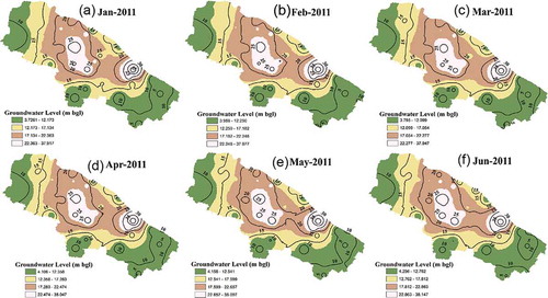
The space–time prediction models were prepared using the hybrid models of geostatistical kriging with the ANN, LS-SVM and GP models. For the prediction, 35 monitoring well sites (the same sites as used in the spatial model) were used for calibrating the models. The datasets of five well sites were used for testing purposes (the same sites as used in the spatial model). Experimental semi-variogram points corresponding to groundwater levels showed an increasing trend with lag distance. Thus, a combination of the nugget effect and power model was utilized as the theoretical variogram model. Table 4 gives the semi-variogram structures for the different hybrid models. Figure 7(a)–(c) shows the experimental semi-variograms fitted with the combination of models. These hybrid models predicted the groundwater level for the testing well sites for the testing period January–June 2011. Spatial maps (Figs. 8, 9 and 10) were drawn for each one-month ahead water level to identify the variation in the results predicted by different space–time models. The training and testing errors obtained for the three temporal models and one spatial model are presented in Tables 2 and 3, respectively. Performance indicators obtained for different space–time models are presented in Table 5. The hybrid model of geostatistical kriging and GP (GP–kriging) shows the lowest AARE, RMSE, NMBE and NRMSE errors and the maximum correlation coefficient (R) values for most of the months compared with the other hybrid models. The performances by the other hybrid models were not significantly different. Predictability of all the hybrid models was found to be similar.

Table 4. Derived theoretical semi-variogram model.

Semi-variogram type	Semi-variogram structure
Spatial	1 Nug(0) + 10Pow(0.5)

Note:

Table 5. Performance indicators obtained for different space–time models.

Month	Performance indicators
	ANN–kriging						LS-SVM–kriging						GP–kriging
	AARE	RMSE	R	E	NMBE	NRMSE	AARE	RMSE	R	E	NMBE	NRMSE	AARE	RMSE	R	E	NMBE	NRMSE
Jan 11	1.8691	2.2152	0.8987	0.7788	0.2969	0.0201	1.8116	2.1863	0.9033	0.7845	0.2498	0.0198	1.834	2.2166	0.9008	0.7785	0.2364	0.0201
Feb 11	2.041	2.4176	0.8811	0.7423	0.3244	0.0219	1.9994	2.3497	0.8851	0.7565	0.2967	0.0213	2.0607	2.3956	0.8791	0.7469	0.3234	0.0217
Mar 11	1.9744	2.2992	0.8959	0.7702	0.4929	0.0209	1.9448	2.2326	0.8991	0.7833	0.4768	0.0203	1.939	2.2138	0.8984	0.787	0.4131	0.0201
Apr 11	2.0595	2.3528	0.8937	0.7682	0.619	0.0214	2.1117	2.4455	0.8885	0.7496	0.6669	0.0222	1.9735	2.2383	0.8999	0.7902	0.4733	0.0204
May 11	2.0284	2.3584	0.9019	0.7688	0.8577	0.0215	2.1476	2.5672	0.8899	0.726	0.9653	0.0234	1.9139	2.2014	0.9094	0.7986	0.6602	0.0201
Jun 11	2.0227	2.3816	0.8947	0.7481	0.8032	0.0217	2.2176	2.6947	0.8749	0.6775	0.9441	0.0246	1.9063	2.2079	0.9018	0.7835	0.5084	0.0201

Figure 7. Examples of experimental semi-variograms for June 2011 fitted with the combination of the nugget effect and power model for different spatio-temporal models: (a) ANN–kriging, (b) LS-SVM–kriging, and (c) GP–kriging.

Figure 8. Spatial maps obtained for the study area from the ANN–kriging model.

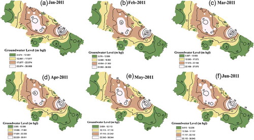
Figure 9. Spatial maps obtained for the study area from the LS-SVM–kriging model.

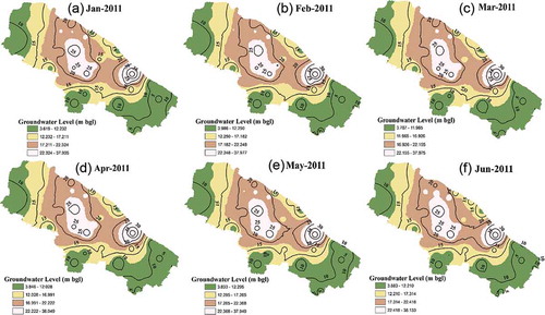
Figure 10. Spatial maps obtained for the study area from the GP–kriging model.

5 Conclusions

In order to identify the best space–time model for groundwater level forecasting in the study area, three hybrid models were developed. Kriging in conjunction with ANN, LS-SVM and GP models was used to develop three space–time models. The ANN and LS-SVM models used optimization techniques that cannot guarantee global optimum solutions. The solutions can be expected to be very close to the global optimum. On the other hand, GP does not use any optimization techniques; it uses a tree structure to present each expression, and finds the best individual tree structure over a number of generations that can most accurately define the target output. The spatial variation of the groundwater levels throughout the study area was interpreted by kriging. The space–time models developed in the present study were compared with each other. Space–time models predicted one-month ahead groundwater level for the study area. Spatial maps were developed using these predicted values. The maps thus prepared showed very little variation in their groundwater level pattern. The efficiency of the models was then judged from the performance indicators: average absolute relative error (AARE), root mean square error (RMSE), correlation coefficient (R), coefficient of efficiency (E), normalized mean bias error (NMBE) and normalized root mean square error (NRMSE). All the models showed nearly equal errors, which suggests that all the models developed for the present study were almost equally efficient. However, the most satisfactory results were obtained for the GP–kriging model, with the lowest AARE, RMSE, NMBE and NRMSE and the maximum R values for most months compared with the other hybrid models. The evaluation results with the small dataset available demonstrate the potential applicability of the proposed framework for predicting space–time groundwater levels.

Disclosure statement

No potential conflict of interest was reported by the authors.

References

- Ahmadi, S.H. and Sedghamiz, A., 2007. Geostatistical analysis of spatial and temporal variations of groundwater level. Environmental Monitoring and Assessment, 129, 277–294. doi:10.1007/s10661-006-9361-z
- Babovic, V. and Keijzer, M., 2002, Rainfall runoff modelling based on genetic programming. Nordic Hydrology, 33, 331–343.
- Bhagwat, P.P. and Maity, R., 2012, Multistep-ahead river flow prediction using LS-SVR at daily scale. Journal of Water Resource and Protection, 2012 (4), 528–539. doi:10.4236/jwarp.2012.47062
- Bhagwat, P.P. and Maity, R., 2013, Hydroclimatic streamflow prediction using least square-support vector regression. ISH Journal of Hydraulic Engineering, 19 (3), 320–328. doi:10.1080/09715010.2013.819705
- Bhat, S., et al., 2015, Geostatistics-based groundwater-level monitoring network design and its application to the Upper Floridan aquifer, USA. Environmental Monitoring and Assessment, 187 (1), 4183. doi:10.1007/s10661-014-4183-x
- Chung, J.W. and Rogers, J.D., 2012, Interpolations of groundwater table elevation in dissected uplands. Ground Water, 50 (4), 598–607. doi:10.1111/j.1745-6584.2011.00889.x
- Daliakopoulos, I.N., Coulibaly, P., and Tsanis, I.K., 2005. Groundwater level forecasting using artificial neural networks. Journal of Hydrology, 309, 229–240. doi:10.1016/j.jhydrol.2004.12.001
- Dash, N.B., et al., 2010. Hybrid neural modeling for groundwater level prediction. Neural Computing and Applications, 19, 1251–1263. doi:10.1007/s00521-010-0360-1
- Dhar, A., 2013, Geostatistics-based design of regional groundwater monitoring framework. ISH Journal of Hydraulic Engineering, 19 (2), 80–87. doi:10.1080/09715010.2013.787713
- Dhar, A., Sahoo, S., and Sahoo, M., 2015. Identification of groundwater potential zones considering water quality aspect. Environmental Earth Sciences, 74, 5663–5675. doi:10.1007/s12665-015-4580-7
- Fallah-Mehdipour, E., Haddad, O.B., and Marino, M.A., 2013, Prediction and simulation of monthly groundwater levels by genetic programming. Journal of Hydroenvironment Research, 7, 253–260.
- Goovaerts, P., 1997. Geostatistics for natural resources evaluation. New York: Oxford University Press.
- Haykin, S., 1994. Neural networks. New York: Macmillan College Publishing Company.
- Hwang, S.H., Ham, D.H., and Kim, J.H., 2012, Forecasting performance of LS-SVM for nonlinear hydrological time series. KSCE Journal of Civil Engineering, 16 (5), 870–882. doi:10.1007/s12205-012-1519-3
- Isaaks, E.H. and Srivastava, R.M., 1989. An introduction to applied geostatistics. New York: Oxford University Press.
- Jain, A. and Srinivasulu, S., 2004. Development of effective and efficient rainfall runoff models using integration of deterministic, real-coded genetic algorithms and artificial neural network techniques. Water Resources Research, 40, W04302. doi:10.1029/2003WR002355
- Jha, M.K. and Sahoo, S., 2015. Efficacy of neural network and genetic algorithm techniques in simulating spatio-temporal fluctuations of groundwater. Hydrological Processes, 29, 671–691. doi:10.1002/hyp.v29.5
- JNNURM, 2006. Kanpur City development plan. Jawaharlal Nehru National Urban Renewal Mission (JNNURM). JPS Associates (P) Ltd. Consultants. Available from: http://jnnurm.nic.in/wp-content/uploads/2010/12/CDP_Kanpur.pdf [ Accessed 22 May, 2014].
- Kholghi, M. and Hosseini, S.M., 2009. Comparison of groundwater level estimation using neuro-fuzzy and ordinary kriging. Environmental Modeling & Assessment, 14, 729–737. doi:10.1007/s10666-008-9174-2
- Kitanidis, P.K., 1997. Introduction to geostatistics: applications in hydrogeology. Cambridge: Cambridge University Press.
- Lallahem, S., et al., 2005. On the use of neural networks to evaluate groundwater levels in fractured media. Journal of Hydrology, 307, 92–111. doi:10.1016/j.jhydrol.2004.10.005
- Machiwal, D., et al., 2012, Modelling short-term spatial and temporal variability of groundwater level using geostatistics and GIS. Natural Resources Research, 21 (1), 117–136. doi:10.1007/s11053-011-9167-8
- Nash, J.E. and Sutcliffe, J.V., 1970, River flow forecasting through conceptual models part I - A discussion of principles. Journal of Hydrology, 10 (3), 282–290. doi:10.1016/0022-1694(70)90255-6
- Nayak, P.C., Rao, Y.R.S., and Sudheer, K.P., 2006. Groundwater level forecasting in a shallow aquifer using artificial neural network approach. Water Resources Management, 20, 77–90. doi:10.1007/s11269-006-4007-z
- Nourani, V., Mogaddam, A.A., and Nadiri, A.O., 2008. An ANN-based model for spatiotemporal groundwater level forecasting. Hydrological Processes, 22, 5054–5066. doi:10.1002/hyp.v22:26
- Samsudin, R., Saad, P., and Shabri, A., 2011. River flow time series using least squares support vector machines. Hydrology and Earth System Sciences, 15, 1835–1852. doi:10.5194/hess-15-1835-2011
- Shabri, A. and Suhartono, 2012, Streamflow forecasting using least-squares support vector machines. Hydrological Sciences Journal, 57 (7), 1275–1293. doi:10.1080/02626667.2012.714468
- Sheta, A.F. and Mahmoud, A., 2001. Forecasting using genetic programming. In Proceedings of the 33rd Southeastern symposium on system theory. Athens, OH, 343–347. doi:10.1109/SSST.2001.918543
- Shiri, J., et al., 2013. Predicting groundwater level fluctuations with meteorological effect implications- a comparative study among soft computing techniques. Computers & Geosciences, 56, 32–44. doi:10.1016/j.cageo.2013.01.007
- Sreekanth, J. and Datta, B., 2010. Multi-objective management of saltwater intrusion in coastal aquifers using genetic programming and modular neural network based surrogate models. Journal of Hydrology, 343, 245–256. doi:10.1016/j.jhydrol.2010.08.023
- Suykens, J.A.K. and Vandewalle, J., 1999. Least squares support vector machine classifiers. Neural Processing Letters, 9, 293–300. doi:10.1023/A:1018628609742
- Ta’any, R., Tahboub, A., and Saffarini, G., 2009, Geostatistical analysis of spatiotemporal variability of groundwater fluctuations in Amman-Zarqa basin, Jordan: a case study. Environmental Geology, 57 (3), 525–535. doi:10.1007/s00254-008-1322-0
- Tapoglou, E., et al., 2014. A spatio-temporal hybrid neural network-kriging model for groundwater level simulation. Journal of Hydrology, 519, 3193–3203. doi:10.1016/j.jhydrol.2014.10.040
- Trichakis, I.C., Nikolos, I.K., and Karatzas, G.P., 2011, Artificial Neural Network (ANN) based modelling for karstic groundwater level simulation. Water Resources Management, 25 (4), 1143–1152. doi:10.1007/s11269-010-9628-6
- Varouchakis, E.A. and Hristopulos, D.T., 2013a. Improvement of groundwater level prediction in sparsely gauged basins using physical laws and geographic features as auxiliary variables. Advances in Water Resources, 52, 34–49. doi:10.1016/j.advwatres.2012.08.002
- Varouchakis, E.A. and Hristopulos, D.T., 2013b. Comparison of stochastic and deterministic methods for mapping groundwater level spatial variability in sparsely monitored basins. Environmental Monitoring Assessment, 185, 1–19. doi:10.1007/s10661-012-2527-y
- Wang, W., et al., 2009. A comparison of performance of several artificial intelligence methods for forecasting monthly discharge time series. Journal of Hydrology, 374, 294–306. doi:10.1016/j.jhydrol.2009.06.019
- Wang, W., et al., 2006. Forecasting daily streamflow using hybrid ANN models. Journal of Hydrology, 324, 383–399. doi:10.1016/j.jhydrol.2005.09.032
- Wong, W.K., Xia, M., and Chu, W.C., 2010. Adaptive neural network model for time-series forecasting. European Journal of Operational Research, 201, 807–816. doi:10.1016/j.ejor.2010.05.022