Hydrological simulation of the Betwa River basin (India) using the SWAT model

ABSTRACT

A seasonal water budget analysis was carried out to quantify various components of the hydrological cycle using the Soil and Water Assessment Tool (SWAT) model for the Betwa River basin (43 500 km²) in central India. The model results were satisfactory in calibration and validation. The seasonal water budget analysis showed that about 90% of annual rainfall and 97% of annual runoff occurred in the monsoon season. A seasonal linear trend analysis was carried out to detect trends in the water balance components of the basin for the period 1973–2001. In the monsoon season, an increasing trend in rainfall and a decreasing trend in ET were observed; this resulted in an increasing trend in groundwater storage and surface runoff. The winter season followed almost the same pattern. A decreasing trend was observed in summer season rainfall. The study evokes the need for conservation structures in the study area to reduce monsoon runoff and conserve it for basin requirements in water-scarce seasons.

EDITOR Z.W. Kundzewicz

ASSOCIATE EDITOR F. Hattermann

KEYWORDS:

• Hydrological modelling
• water balance
• Betwa basin
• SWAT model

1 Introduction

The hydrological cycle is a system that is fairly easy to grasp and understand, although it is far from easy to quantify processes in the system. Due to the complexity associated with hydrological processes, numerous models have been developed in the past to assist in understanding the hydrological system (Arnold and Allen 1996). Hydrological models, such as the Areal Non-Point Source Watershed Environment Response Simulation (ANSWERS; Beasley et al. 1977), Agricultural Non-Point Source Pollution (AGNPS; Young et al. 1995), Water Erosion Prediction Project (WEPP; Laflen et al. 2004) and Soil and Water Assessment Tool (SWAT; Arnold et al. 1993) are used extensively for water resources management. Among them, the SWAT model has been used extensively by several researchers globally in the past (Srinivasan et al. 1993, 1998, Srinivasan and Arnold 1994, Cho et al. 1995, Rosenthal et al. 1995, Peterson and Hamlett 1998, Cao et al. 2006, Rouhani et al. 2007, Thampi et al. 2010, El-Sadek et al. 2011, Murty et al. 2014) and this model has shown promising results.

The SWAT model underlies the ArcSWAT interface, in which ArcGIS is used to provide a geographical analysis that is fed into the SWAT model and provides hydrological outputs. Tripathi et al. (1999a, 1999b) estimated the daily and monthly runoff and sediment yield from the Nagwan watershed in Eastern India using the SWAT model. Shrivastava et al. (2004) tested the SWAT model on a daily and a monthly basis for estimating surface runoff and sediment yield from a small watershed, Chhokeranala in eastern India. Li et al. (2009) used the SWAT model satisfactorily in the upper reaches of the Heihe River basin in China. Rouhani et al. (2007) calibrated and validated the SWAT model with respect to the total flow and low flow. Their study revealed that SWAT is unbiased for high and low flows. Cao et al. (2006) adopted a multi-variable and multi-site approach for calibration and validation of the SWAT model for the Motueka catchment in New Zealand. Thampi et al. (2010) applied the SWAT model to the 2530 km² Chaliyar River basin in Kerala, India, to investigate the influence of scale on the model parameters. The results indicated that there may be greater uncertainty in SWAT streamflow estimates as the size of the watershed increases.

Hydrological models offer an inexpensive tool to analyse the performance of a hydrological system. Different hydrological variables (e.g. contribution of baseflow/interflow, interception etc.) may be difficult to obtain; therefore, models are employed to generate them. In the present study, the SWAT model has been used to study and quantify the seasonal water balance of the Betwa River basin, India, for which only monthly streamflow data are available. The SWAT model is a process-based, spatially-distributed and continuous model capable of simulating water balance, taking into account rainfall, evapotranspiration, surface and subsurface runoff and deep aquifer recharge; runoff partitioning into surface and subsurface runoff is based on the curve number (CN) method and a kinematic percolation model (Arnold et al. 1998, Nunes and Seixas 2011).

A river basin is a hydrologically self-contained area and a natural unit for water resources planning (National Water Policy 2012). Therefore, understanding the water balance of a basin is of profound importance. The catchment area of the Betwa River basin falls under the jurisdiction of two states: Uttar Pradesh and Madhya Pradesh in India. The population of Uttar Pradesh (approx. 199 million) is the highest of the states in India, with a growth rate of 20.10% in the period 2001–2011. The population of Madhya Pradesh (approx. 72 million) is greater than the combined population of Afghanistan, Australia and Sri Lanka. In the last decade (2000–2010), Madhya Pradesh has added a population of more than that of Greece, with a growth rate of 20.30% (Census of India 2011). The increasing population of these states is pushing the natural limits of the water resources to alarmingly low levels. The ability to meet the fundamental needs of the populations and ensure environmental protection will be increasingly threatened if water resources are not managed properly. The region, though historically important, continues to be highly underdeveloped due to poor management of irrigation facilities. The rainfall is scanty, uncertain and unevenly distributed; land degradation has taken place and may further increase due to continuing deforestation (Chaube et al. 2011, Suryavanshi et al. 2014). Fertile alluvial plains in the north coupled with irregular famines have resulted in great demand for more accurate measurements of rainfall and discharge (Ahlawat 2010).

It is evident that limited information on application of the SWAT model for basin-level study is available for the Indian context in general and the Betwa River basin in particular. In India, topographical conditions, soil conditions, rainfall patterns and cultivation practices are different from those in the other parts of the world (Pandey et al. 2008). Therefore, it is important to evaluate physically-based models such as SWAT for Indian basins. Hence, the present study was carried out with the explicit objective of calibration, sensitivity analysis, validation and evaluation of the SWAT model for analysing the water balance components under Indian conditions for the Betwa basin.

2 Materials and methods

2.1 Study area

The Betwa basin (77°10ʹ–80°20ʹE; 22°54ʹ–26°05ʹN), located in central India, was selected as the study area (Fig. 1(a)). Its elevation ranges from 106 to 706 m above mean sea level (a.m.s.l.).

Figure 1. (a) Location map of the Betwa basin and (b) location of meteorological stations in the basin.

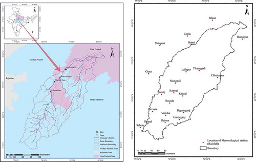
The Betwa River originates near Barkhera village in the Raisen district of Madhya Pradesh at about 576 m a.m.s.l. and discharges into the Yamuna River near Hamirpur in Uttar Pradesh at about 106 m a.m.s.l. The total length of the river from its origin to confluence is 590 km, of which 232 km lies in Madhya Pradesh and the remaining 358 km in Uttar Pradesh. The climate of the Betwa basin is moderate, the air being mostly dry except during the southwest monsoons (Chaube 1988). The Agricultural Informatics Division of the National Informatics Centre, Ministry of Information and Communication Technology, Government of India (http://dacnet.nic.in) has proposed wheat, paddy, maize and sorghum as the most suitable crops in the region.

2.2 Data collection and analysis

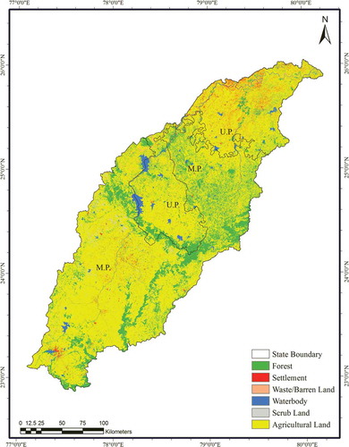
Historical daily rainfall data for 28 years (1973–2001) were collected (IMD, Pune and State Data Centre, Bhopal) from 18 raingauge stations (Chhatarpur, Hamirpur, Jalaun, Shivpuri, Jhansi, Tikamgarh, Banda, Bhopal, Raisen, Vidisa, Basoda, Begumganj, Berasia, Chanderi, Khurai, Kurwai, Mungauli and Sironj) located in the Betwa basin (Fig. 1(b)). Other meteorological data, including maximum and minimum air temperature, solar radiation, relative humidity and minimum and maximum sunshine hours, were collected from different meteorological observatories. Beside these, discharge data (monthly basis) at the outlet of the Basoda gauging site (1980–2001) and the Rajghat gauging site (1980–1985) were also collected from the State Data Centre, Bhopal. Cloud-free digital data from Landsat imagery with 30 m spatial resolution (http://glcf.umd.edu/data/) for the year 2001 were used to generate the land-use/land-cover map of the Betwa basin. The Landsat data were in three electromagnetic spectral bands (Band 1: 0.63–0.69 μm; Band 2: 0.75–0.90 μm; and Band 3: 1.55–2.35 μm). The supervised classification, one of the most common land-use classification methods, was used in this study. The classification was carried out using ground control points, collected with the help of hand-held GPS during field visits to the river basin in November 2010. Each pixel in the image dataset was then categorized into the land-use class it most closely resembled. Overall classification accuracy and kappa coefficient (κ) of 78.11% and 0.74, respectively, were obtained in the present study. The classified land-use/land-cover classes were forest, waste/barren land, scrubland, agricultural land, settlements and water body. The area occupied by each land-use/land-cover class is presented in Figure 2.

Figure 2. Land-use map of the Betwa basin.

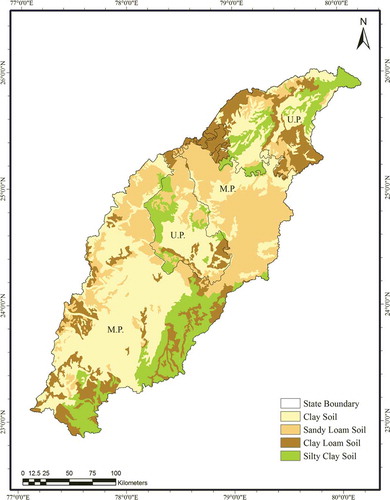
The Betwa basin falls under the Vindhyan Sandstone, Deccan Traps and Bundelkhand Granite. Based on the data obtained from National Bureau of Soil Survey and Land Use Planning (NBSSLUP), Nagpur, soils of the basin are classified as Clay, Silty Clay, Clay Loam and Sandy loam (Fig. 3). The physical and chemical properties of the soils are taken from Soils of Madhya Pradesh (NBSS publication 59) and are presented in Table 1. In this study, Advanced Space-borne Thermal Emission and Reflection (ASTER), elevation data were used for topographical analysis of the basin.

Table 1. Physical and chemical properties of the soils in the Betwa basin. MBD: moist bulk density; OCC: organic carbon content; SHC: soil hydraulic conductivity.

Soil property	Clay				Clay loam		Sandy loam		Silty clay
	Layer 1	Layer 2	Layer 3	Layer 4	Layer 1	Layer 2	Layer 1	Layer 2	Layer 1	Layer 2	Layer 3	Layer 4	Layer 5	Layer 6
Depth (mm)	140	280	280	600	60	80	100	120	110	290	300	350	300	350
MBD (Mg/m^3)	1.32	1.43	1.48	1.53	1.47	1.71	1.70	1.70	1.35	1.43	1.53	1.57	1.58	1.58
OCC (%)	0.70	0.60	0.50	0.20	1.65	1.56	1.42	1.36	0.48	0.36	0.30	0.24	0.24	0.21
Clay (%)	52.10	55.30	64.20	65.10	34.20	37.1	14.20	35.70	46.40	48.60	49.80	48.30	43.1	38.50
Silt (%)	32.30	27.30	27.10	19.80	38.10	22.40	22.30	20.70	43.20	44.80	45.80	44.30	50.20	48.10
Sand (%)	15.60	17.00	8.70	15.10	22.70	40.50	63.50	43.60	10.40	6.66	4.20	7.40	6.70	13.40
SHC (mm/h)	11.45	11.45	11.45	5.60	29.50	29.50	10.40	10.40	12.10	12.10	12.10	4.30	4.30	4.30
USLE K factor	0.20	0.17	0.12	0.12	0.28	0.26	0.55	0.30	0.25	0.24	0.23	0.24	0.29	0.34

Figure 3. Soil map of the Betwa basin.

2.3 SWAT model set-up for the Betwa basin

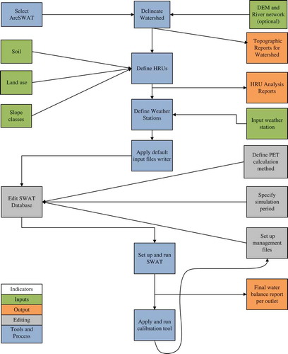
The SWAT model set-up was carried out using ArcSWAT2009.93.7a software (Fig. 4). The interface helped in watershed parameterization and model input. The input parameters of the model were extracted from the satellite imagery, DEM analysis, soil maps and field observations. The stream network was generated by use of a threshold area that defines the origin of a stream. The delineation scheme with moderate level of subdivision gives the best modelling efficiency (Gong et al. 2010). In this study, the threshold value is considered as 12 000 ha. Hydrological response units (HRUs) were created using land-use/land-cover, soil and slope layers. A total of 35 sub-basins and 2717 HRUs were created. For the entire Betwa River basin, 15 weather stations were used for climatic data input. Sensitivity analysis was performed to determine key parameters required for calibration. Sensitivity analysis was conducted using a combined method of the Latin hypercube one-factor-at-a-time (LH-OAT) method, as proposed by Morris (1991). The monthly calibration was carried out using manual adjustment of input parameters to attain satisfactory agreement between simulated and observed discharge data (1980–1990). Simulation accuracy was checked using a validation process. In this process, the model was operated with input parameters set during the calibration process without any further change, and the results were analysed with the remaining observational data. The model was validated with observed discharge data from the Basoda gauging site (1991–2001). Ideally, for large river basins the validation process has to be multi-site. Thus, the model was also validated at the Rajghat site for January 1980 to July 1985.

Figure 4. Workflow diagram for set-up and running of the SWAT model (Lewarne 2009).

2.4 Criteria for model evaluation

For scientifically sound model calibration and validation, a combination of different efficiency criteria is recommended (Krause et al. 2005). In this study, the following statistical criteria were used to evaluate model performance: the coefficient of determination, R² (Willmot 1981, Legates and McCabe 1999); the Nash-Sutcliffe efficiency coefficient, E_NS (Nash and Sutcliffe 1970); the index of agreement, d (Willmot 1981); modified forms of the Nash-Sutcliffe coefficient, E, and index of agreement, d1, (Krause et al. 2005); percentage bias, PBIAS (Gupta et al. 1999); and root mean square error (RMSE) of observations standard deviation ratio, RSR (Legates and McCabe 1999, Chu and Shirmohammadi 2004, Singh et al. 2004, Vasquez-Amabile and Engel 2008), as given by Equations (1)–(7), respectively, where Y_i^obs is the ith observed data point, is the mean of observed data, Y_i^sim is the ith simulated value, is the mean model simulated value, and N is the total number of events:

(1)

(2)

(3)

(4)

(5)

(6)

(7)

3 Results and discussion

3.1 Model pre-calibration

The pre-calibrated model results for runoff are presented in Figure 5. The values of the pre-calibrated runoff hydrograph (Fig. 5) are continuously under-predicted compared to the measured runoff hydrograph for all the years of simulation. The observed and simulated monthly runoff values for the pre-calibration period (along with the 1:1 line) are presented in Figure 6. It is observed that the simulated runoff values are distributed almost continuously below the 1:1 line (Fig. 6), indicating that the model under-predicts the values of runoff (except for some small flow values). Although the value of R² (Table 2) is quite high (0.91), it has to be noted that R² estimates the combined dispersion against the single dispersion of the observed and predicted series, which is one of the major drawbacks of R² if it is considered alone. A model that systematically over- or under-predicts all the time will still result in good R² values close to 1.0, even if all its predictions are wrong (Krause et al. 2005).

Table 2. Statistical analysis of observed and simulated monthly discharge (pre-calibrated) at Basoda for the period 1980–1990.

Statistical parameter	Discharge (m^3/s)
	Observed	Simulated
Mean	213.96	152.64
Standard deviation, SD	311.91	236.54
Maximum	1447.60	1126
Count	132	132
Coefficient of determination, R^2	0.91
Nash-Sutcliffe efficiency, ENS	0.77
Index of agreement, d	0.92
Modified Nash-Sutcliffe coefficient, E	0.37
Modified index of agreement, d1	0.76
Percentage bias, PBIAS	30.44
RMSE-observations standard deviation ratio, RSR	0.47

Figure 5. Pre-calibrated observed and simulated monthly discharge at Basoda for the period 1980–1990.

Figure 6. Comparison between the pre-calibrated observed and simulated monthly discharge at Basoda for the period 1980–1990.

For pre-calibrated runoff, E_NS was calculated as 0.77, which is fairly high and can be judged a good result. However, the largest disadvantage of E_NS is that the differences between observed and predicted values are calculated as squared values. As a result, larger values in a time series are strongly overestimated, whereas lower values are neglected (Legates and McCabe 1999). For the quantification of runoff predictions this leads to an overestimation of model performance during peak flows and an underestimation during low-flow conditions. Similar to R², the E_NS is not very sensitive to systematic model over- or under-prediction, especially during low-flow periods (Krause et al. 2005). The value of d was calculated as 0.92, which is quite high for a pre-calibrated model. Krause et al. (2005) suggested that relatively high values of d (> 0.65) may be obtained even for poor model fits because d is not sensitive to systematic model over- or under-prediction. To overcome the insensitivity of E_NS, R² and d, several other evaluation criteria were selected, such as E and d1, PBIAS and RSR.

In the present study, the input parameters required by the model were obtained from direct field and laboratory measurements, the literature (Neitsch et al. 2004), remote sensing, GIS and through the calibration process of the models, where selected model parameters were adjusted within a required range and the discrepancies between the measured and model predictions could be minimized (Donigian and Rao 1990). Parameters such as plant uptake compensation factor, soil evaporation compensation factor, groundwater delay, and effective hydraulic conductivity in the main channel alluvium were taken into consideration for calibration of the model. Different values between the lower and upper limits were chosen and the model was run to simulate runoff. Since many of the input parameters were available for the basin, they were not calibrated (Suryavanshi 2012).

3.2 Sensitivity analysis

In this study, a LH-OAT method, which is incorporated in the model, was used to perform sensitivity analysis. The analysis was carried out based on the objective function of the SSQ (sum of the squares of the residuals) for 26 model parameters and 10 intervals of LH sampling. After set-up of the SWAT model and incorporation of all the input parameters, simulations and sensitivity analysis were carried out for the years 1976–2001. The results indicate the parameters that were the most crucial for the study area, namely: curve number (CN), soil evaporation compensation factor (ESCO), soil available water capacity (SOL_AWC), soil depth (SOL_Z), threshold depth of water in the shallow aquifer for “revap” (REVAPMN), threshold depth of water in the shallow aquifer required for return flow (GWQMN), effective hydraulic conductivity in main channel (Ch_K₂), groundwater recession factor (ALPHA_BF), plant uptake compensation factor (EPCO), Manning’s n for the main channel (CH_N₂), groundwater delay time (GW_DELAY), surface runoff lag coefficient (SURLAG), saturated hydraulic conductivity (SOL_K) and groundwater revap coefficient (GW_REVAP) (Table 3).

Table 3. Sensitivity ranking of the SWAT model parameters.

Parameter	Sensitivity rank
CN	1
ESCO	2
SOL_AWC	3
SOL_Z	4
REVAPMN	5
GWQMN	6
CH_K2	7
ALPHA_BF	8
EPCO	9
CH_N2	10
GW_DELAY	11
SURLAG	12
SOL_K	13
GW_REVAP	14

Sensitivity analysis indicated the overall importance of all parameters in determining the runoff of the study area. Parameters CN, EPCO, ESCO, ALPHA_BF and GW_DELAY were found to be the most sensitive parameters towards the model outputs. All the parameters generally govern the surface and subsurface hydrological processes and stream routing. These results illustrate how parameter sensitivity is site specific and depends on land use, topography and soil types compared to other studies.

3.3 Model calibration

The successful application of a hydrological model depends on how well the model is calibrated (Gupta et al. 1999). In this study, manual calibration was performed for the Betwa River basin using observed monthly runoff measured at the Basoda outlet for the years 1980–1990. The first 3 years (1973–1975) of the modelling period were reserved for model “warm-up” in order to make a model to realistically set-up the states of its internal hydrological compartments, i.e. groundwater storage, soil moisture content, etc. Parameters were modified by replacement, by addition of an absolute change, and by multiplication of a relative change depending on the nature of the parameter. However, a parameter was never allowed to go beyond the pre-defined absolute parameter ranges during the calibration process.

Manual calibration involves manual adjustment of the SWAT model parameters through a trial-and-error approach, until acceptable simulation is achieved. The input variables used for model calibration were: CN, EPCO, ESCO, ALPHA_BF, GW_DELAY, Ch_K₂, Manning’s n for the main channel and SURLAG (Table 4).

Table 4. Parameters used for calibration of the SWAT model.

Parameter	Range	Value taken	Process
Curve number, CN	35–98	5% increase	Runoff
Plant uptake compensation factor, EPCO	0–1	0.90	Evaporation
Soil evaporation compensation factor. ESCO	0–1	0.85	Evaporation
Baseflow alpha factor, ALPHA_BF	0–1	0.50	Groundwater
Groundwater delay time, GW_DELAY	0–50	15	Groundwater
Effective hydraulic conductivity in main channel alluvium, CH_K2	0.01–150	25	Channel
Manning’s n for the main channel (CH_N2)	0.008–30	0.025	Channel
Surface runoff lag coefficient (SURLAG)	0–10	2	Runoff

As land-use/land-cover change is not considered in this study, adjustments were made to the CN values to account for land-use and land-cover changes. The SCS curve number is one of the driving factors for land use, soil permeability and antecedent soil moisture conditions. It has been observed that increasing CN decreases infiltration and baseflow and thus increases hydrograph spikes. For this study, a 5% increment was considered for CN.

The amount of water consumed by a plant depends on the amount of water required by the plant for evapotranspiration (ET) and the amount of water available in the soil. If the upper layers in the soil profile do not contain enough water to meet the potential water uptake, the model allows lower layers to compensate (Neitsch et al. 2004). The plant uptake compensation factor (EPCO) ranges from 0.01 to 1. As EPCO approaches 1, the model allows water uptake demand to be met by lower layers in the soil. In this study, the chosen value of EPCO was 0.90.

The soil evaporation compensation factor (ESCO) allows the user to modify the distribution used to meet soil evaporated demand to account for the effect of capillary action, crusting and cracks. Normal values of ESCO range between 0.01 and 1. The calibrated value of ESCO was 0.85. It was observed that the higher the value of ESCO, the lesser evaporation and hence more runoff.

The baseflow recession constant (ALPHA_BF) is a direct index of groundwater flow response to changes in recharge (Smedema and Rycroft 1983). The baseflow alpha ranges between 0 and 1. The calibrated baseflow value of the alpha factor was 0.50. However, during calibration of the model, it was observed that, with the increase in ALPHA_BF, there was an increase in the runoff, particularly during peak flow. However, baseflow was reduced considerably during the dry season.

Water that moves past the lowest depth of the soil profile by percolation or bypass flow enters and flows through the vadose zone before becoming shallow aquifer recharge (Neitsch et al. 2004). Groundwater delay time (GW_DELAY) is the time lag between water exiting the soil profile and entering the shallow aquifer. It depends on depth to the water table and the hydraulic properties of the geological formations in the vadose and groundwater zones. During calibration of the model, it was observed that a lower value of GW_DELAY indicated the smooth small contribution of groundwater to baseflow and thus increased surface runoff. The calibrated value of GW_DELAY was found to be 15 days.

Lane (1983) suggested hydraulic conductivity values for various bed materials. Accordingly, the present study area falls under Category 4 (Moderate loss rate), with bed material characteristics of high silt–clay content. Keeping this in mind, the calibrated value of hydraulic conductivity was considered to be 25 mm/h.

The value of Manning’s n is determined from the values of factors that affect the roughness of channels and flood plains. During field visits on November 2010, it was observed that the flood channel was covered with a few trees, stones and brush. The value of Manning’s n for the main channel for a natural stream with few trees, stones or brush is between 0.025 and 0.065 (Chow 1959). The calibrated value of n was 0.025.

The Betwa River basin has a large sub-basin area. The time of concentration in such a river basin is generally greater than 1 day (only a portion of the surface runoff will reach the main channel on the day it is generated). For a given time of concentration, as the surface runoff lag coefficient (SURLAG) decreases, more water is held in storage. The delay in release of surface runoff will smooth the streamflow hydrograph simulated in the reach. The calibrated value for SURLAG was 2.

For calibration of the SWAT model, observed monthly streamflow data obtained at the Basoda site (outlet no. 29) were compared with the model simulated streamflow data (Figs 7 and 8). For calibration purposes, model simulation was performed for an 11-year period (1980–1990). It is seen in Figure 7 that the peak values of the simulated runoff for the years 1982, 1983, 1986 and 1987 generally match the observed runoff closely, although often at different magnitudes. During the initial stages of the monsoon (1987/88), the model over-predicted the runoff, whereas, after advancement of the monsoon, the model slightly under-predicted runoff (1980, 1981, 1984, 1988–1990). This may be due to (a) overestimation of the baseflow during the early monsoon, and (b) slightly lower assignment of CN. Other possible reasons for lower prediction of runoff may be the lower density of meteorological stations (data) at higher-altitude areas from which higher runoff is generally expected. Understandably, climate information represents the main forcing data for a hydrological model (Hattermann et al. 2005). The observed and simulated monthly runoff for the calibration period (along with the 1:1 line) are shown in Figure 8. It can be observed that the simulated runoff values are distributed uniformly about the 1:1 line for lower values of observed runoff (Fig. 8). For high values of observed runoff, simulated values are slightly below the 1:1 line, indicating that the model under-predicts the high values of runoff. A high value (0.88) of R² indicates a close relationship between the observed and simulated runoff. Further, the efficiency of the model for simulated runoff was tested by statistical analysis, as presented in Table 5. A high value of E_NS of 0.87 indicates that there is a good agreement between the observed and simulated runoff during the calibration period. The ranges of d, E and d1 are similar to that of R² and lie between 0 (no correlation) and 1 (perfect fit), with values of 0.97, 0.78 and 0.91, respectively. The optimal value of PBIAS is 0.0, with low values indicating accurate model simulation. Positive values indicate model under-estimation bias, and negative values indicate model over-estimation bias (Gupta et al. 1999). In this study, the value of PBIAS was found to be 4.11. According to Van Liew et al. (2007), this value is rated as “very good” for calibration. The RSR varies from the optimal value of 0, which indicates zero RMSE or residual variation and, therefore, perfect model simulation, to a large positive value. The lower the value of RSR, the lower is the RMSE and the better is the model simulation performance (Krause et al. 2005). After calibration, the RSR value was found to be 0.35, which is a “very good” rating. Thus, the results indicate that the overall prediction of monthly surface runoff by the SWAT model for the calibration period was satisfactory and, therefore, could be accepted for further analysis.

Table 5. Statistical analysis of observed and simulated monthly discharge (calibrated) at Basoda for the period 1980–1990.

Statistical parameter	Discharge (m^3/s)
	Observed	Simulated
Mean	213.96	215.52
Standard deviation, SD	311.91	262.09
Maximum	1447.60	1379
Count	132	132
Coefficient of determination, R^2	0.91
Nash-Sutcliffe efficiency, ENS	0.84
Index of agreement, d	0.95
Modified Nash-Sutcliffe coefficient, E	0.77
Modified index of agreement, d1	0.90
Percentage bias, PBIAS	1.79
RMSE-observations standard deviation ratio, RSR	0.39

Figure 7. Observed and simulated monthly discharge (calibrated) at Basoda for the period 1980–1990.

Figure 8. Comparison between the observed and simulated monthly discharge at Basoda for the period 1980–1990 for model calibration.

3.4 Model validation

In order to utilize the calibrated SWAT model for predicting the water balance, the model was validated on an independent validation period (1991–2001) with observed runoff data for the Basoda gauging site and the Rajghat site (January 1980–July 1985).

3.4.1 Basoda gauging site

The observed and simulated monthly discharges at the Basoda site for the validation period (1991–2001) were compared graphically, as shown in Figure 9. It is evident from Figure 9 that simulated and observed monthly discharges are in good agreement in all 11 years for the Basoda site. The simulated peaks are marginally under-predicted from the measured peaks for the months of August–September 1994, August–September 1996, September 1997 and July 2000, and for the lower magnitudes of discharge the model over-predicted for January–May 1991, January–May 1992, March–May 1998 and March–May 2000. Figure 10 presents scattergrams comparing the simulated discharge with observed values, along with the 1:1 line, for 1991–2001. It can be seen that most of the compared points are evenly distributed for lower magnitudes of discharge, but the simulated values are slightly below the 1:1 line (Fig. 10) for higher discharge values, indicating that the model under-predicted the high values of discharge.

Figure 9. Observed and simulated monthly discharge at Basoda for the period 1991–2001 for model validation.

Figure 10. Comparison between the observed and simulated monthly discharge at Basoda for the period 1900–2001 for model validation.

The descriptive statistics for observed and simulated monthly discharge for all the years are shown in Table 6. At the Basoda site, for model validation the R² and E_NS were found to be 0.91 and 0.88, respectively, which reflects a close agreement between the simulated and observed monthly discharge for the years 1991–2001. The values of d, E and d1 were 0.96, 0.72 and 0.85, respectively.

Table 6. Statistical analysis of observed and simulated monthly discharge at Basoda for the period 1991–2001: model validation.

Statistical parameter	Discharge (m^3/s)
	Observed	Simulated
Mean	240.97	235.88
Standard deviation, SD	351.84	280.59
Maximum	1481.40	1231
Count	132	132
Coefficient of determination, R^2	0.91
Nash-Sutcliffe efficiency, ENS	0.88
Index of agreement, d	0.96
Modified Nash-Sutcliffe coefficient, E	0.72
Modified index of agreement, d1	0.85
Percentage bias, PBIAS	2.11
RMSE-observations standard deviation ratio, RSR	0.33

The value of PBIAS was found to be 2.11, which reflects a very good tendency of data for validation. The RSR was 0.33, which can be termed “very good”.

3.4.2 Rajghat gauging site

The hydrograph of simulated and observed monthly discharge at the Rajghat site for model validation is presented in Figure 11. It can be seen that the peak flow simulated by the SWAT model is slightly lower than the observed discharge for August 1982 and September 1983 (Fig. 11). However, the model over-predicts the lower discharge for March–May 1982 and April–May 1984. Observed and simulated monthly discharge at Rajghat for the validation period, along with the 1:1 line, are shown in Figure 12. The simulated discharge values are distributed uniformly about the 1:1 line for lower values of observed discharge (Fig. 12). For high values of observed discharge, the simulated values are slightly below the 1:1 line, indicating that the model under-predicts the high values of discharge. However, a high value of coefficient of determination (R² = 0.92) indicates a close relationship between observed and simulated discharge.

Figure 11. Observed and simulated monthly discharge at Rajghat for the period January 1980–July 1985 for model validation.

Figure 12. Comparison between the observed and simulated monthly discharge at Rajghat for the period January 1980–July 1985 for model validation.

The descriptive statistics for observed and simulated monthly discharge for all the years are shown in Table 7. At Rajghat, during validation, the values of R² and E_NS were 0.92 and 0.82, respectively, which reflects a close agreement between the simulated and observed monthly discharge for the given years. The values of d, E and d1 were 0.93, 0.54 and 0.68, respectively. The value of PBIAS was 9.89, which reflects a “very good” tendency (PBIAS < ±10) of data for validation. The RSR was 0.41 (0.00 < RSR < 0.50), which is a “very good” rating.

Table 7. Statistical analysis of observed and simulated monthly discharge at Rajghat for the period January 1980–July 1985: model validation.

Statistical parameter	Discharge (m^3/s)
	Observed	Simulated
Mean	405.36	445.49
Standard deviation, SD	939.24	613.35
Maximum	4988.66	3418
Count	67	67
Coefficient of determination, R^2	0.92
Nash-Sutcliffe efficiency, ENS	0.82
Index of agreement, d	0.93
Modified Nash-Sutcliffe coefficient, E	0.54
Modified index of agreement, d1	0.68
Percentage bias, PBIAS	9.89
RMSE-observations standard deviation ratio, RSR	0.41

Thus, satisfactory model performance during validation at both the Basoda and the Rajghat sites encourages the applicability of the SWAT model for analysis of water balancing components of the Betwa basin.

3.5 Water balance analysis of the Betwa basin

Analysis was carried out to evaluate the seasonal and yearly water balance of the Betwa basin for the period 1976–2003 (28 years). For the seasonal water balance analysis, the water year (i.e. 1 June to 31 May) was classified into three seasons of four months each: Season I corresponds to the monsoon season, i.e. June–September; Season II corresponds to the winter season, i.e. October–January; and Season III corresponds to the summer season, i.e. February–May.

The water balance of the Betwa basin, consisting of various components of the simulated hydrological processes in the study area, is presented in Table 8.

Table 8. Seasonal and annual water balance and their linear trends in the basin.

	Rainfall		SURQ		GWQ		ET
	Annual average	Change	Annual average	Change	Annual average	Change	Annual average	Change
	(mm)	(mm/year)	(mm)	(mm/year)	(mm)	(mm/year)	(mm)	(mm/year)
Season I	1016	1.354	395	2.298	159	1.949	413	−3.18
Season II	65	−1.94	9	−0.855	8	−1.22	87	0.45
Season III	42	−0.645	2	−0.001	1	0.003	70	−3.29
Year	1123	−1.232	406	1.442	168	0.731	570	−6.02

3.5.1 Season I: monsoon season

It can be observed from Table 8 and Figure 13 that about 90% (1016 mm) of annual rainfall (1123 mm) occurs during Season I. Of the total yearly runoff of 406.4 mm (which is 36.2% of precipitation), 395.23 mm (97% of total) occurs in the monsoon season.

Figure 13. Water balance for Season I (June–September) in the Betwa basin for 1976–2003.

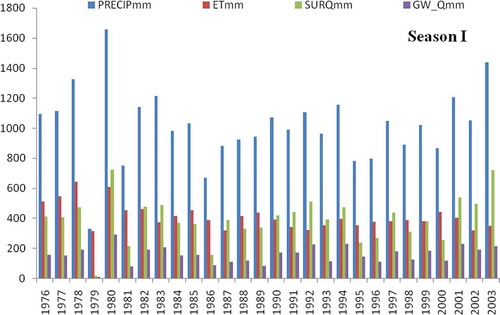
The Betwa is a rain-fed river, so the hydrology of the Betwa basin is greatly influenced by rainfall. The river swells up and floods occur during the rainy season and it dries up in the summer (Betwa River Board 1979). Therefore, if the water is not stored in the monsoon season, famine-like conditions are created during the remaining part of the year. Groundwater percolation was almost 94% of the yearly groundwater contribution. The ET contribution in the monsoon season was found to be 73% of yearly ET. Evapotranspiration has a large impact on water and forest resources and the distribution and abundance of these resources are governed by the volume and seasonality of available moisture (Neilson et al. 1992).

3.5.2 Season II: winter season

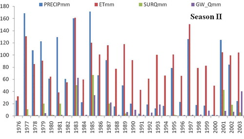
Season II is a lean season with an average rainfall of only 65 mm (Table 8 and Fig. 14). Of this rainfall, runoff is about 15%. The runoff in Season II is about 2% of the yearly runoff. The groundwater contribution is 13.36%, which is only 5% of the yearly groundwater contribution. Being a rain-fed river (with no contribution from glacier-melt runoff), the rabi (winter crop) season is adversely affected due to the reduced availability of water for crops. It should be noted that the geological features of the area and the economic conditions of the people mean that cultivators are unable to install tube wells, shallow wells or tanks using their own resources. The ET contribution in Season II was found to be 15% of the yearly ET.

Figure 14. Water balance for Season II (October–January) in the Betwa basin for 1976–2003.

3.5.3 Season III: summer season

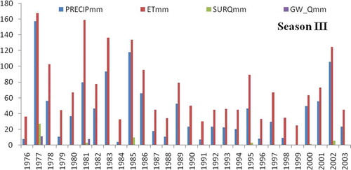
In Season III, the rainfall is scant and uncertain. Only 42 mm of rainfall occurs between February and May (Table 8 and Fig. 15). About 4% of this rainfall is runoff. The runoff in Season III is about 1% of the yearly runoff. Groundwater percolation in Season III is 1.68%, which is only 1% of the yearly groundwater contribution. However, the ET contribution in Season III was about 12% of yearly ET.

Figure 15. Water balance for Season III (February–May) in the Betwa basin for 1976–2003.

3.5.4 Yearly water balance

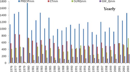
It can be observed that of 1123 mm annual average rainfall, 36% flows out as surface runoff from the study area (Table 8 and Fig. 16). The annual average groundwater contribution is 14%. On average, ET accounts for about 50% of annual precipitation. The Betwa basin is an agriculture-dominated basin (76% of basin area); however, the economic condition of the large population that depends on agriculture remains under-privileged due to agro-climatic conditions and poor management of water resources. Appropriate best management practices such as strip cropping, grassed waterways and vegetative filter strips could be implemented for better water management.

Figure 16. Yearly water balance in the Betwa basin for the period 1976–2003.

3.6 Trend analysis of water balancing parameters using linear regression

A linear trend analysis was carried out (Table 8) to detect trends in different water balance components of the basin in the period 1973–2001. For Season I, an increasing trend was observed in rainfall and a decreasing trend was observed in ET. This increase in rainfall and decrease in ET results in an increasing trend in groundwater storage and surface runoff. In Season II, an increasing trend was observed in ET and a decreasing trend in rainfall, runoff and groundwater contribution. In Season III, a decreasing trend was observed in rainfall. This is reflected in a decreasing trend of ET. The magnitude of changes in runoff and groundwater contribution is very small in Season III and can be neglected and reported as “no trend”. On a yearly basis, it was observed that there is a decreasing trend in rainfall and in ET in the basin, while an increasing trend was observed in runoff and in groundwater contribution. The increase in runoff and groundwater storage was primarily due to reduction in the ET losses from the basin. Explicitly, rainfall and ET are governing factors of surface and groundwater hydrology. Suryavanshi et al. (2014) reported on the annual and seasonal trends of rainfall, the number of rain days, PET and minimum and maximum temperatures for the Betwa basin. They reported that several of the meteorological stations exhibited a decreasing trend in annual and seasonal precipitation, and seasonal and yearly rain days. A number of stations showed an increasing trend in minimum temperature. Their study indicated warmer and dryer conditions in the basin.

3.7 Future scope of the study

To circumvent the problem of uneven distribution of water in the Betwa basin, an ambitious plan has been prepared (in the recent past) for interlinking the Betwa and Ken basins. The Ken–Betwa Link Project (KBLP) is one of the 30 river links proposed by National Water Development Agency (NWDA), which aims to provide additional water to areas in the lower part of the Betwa basin from the adjacent Ken basin. While no links have been built to date, the KBLP is being pursued as the pilot project of a national programme for the interlinking of rivers.

The inter-basin transfer is likely to result in a change in hydrological regime of the Betwa basin. While ambitious plans for interlinking of river basins are debated, there is a need for scientific analysis of the long-term changes likely to result from inter-basin transfer of water. Such studies require thorough understanding of the water balance and climate change in the area. To this end, the present study can be successfully adopted for further analysis of changes in hydrological regimes of the Betwa basin due to river interlinking in a changing climate. The calibrated SWAT model has the efficacy to address a wide range of river basin problems at different spatial and temporal scales. The study on the Betwa basin can further be utilized to study long-term changes in hydro-meteorological variables of the basin, as well as the long-term trends of its water balance components, before and after implementation of the KBLP.

4 Summary and conclusions

In the present study, the SWAT model is appraised to be a fair model for water balance studies in an agriculture-dominated basin. The SWAT model was applied to analyse the seasonal water budget for the Betwa River basin in central India. The under-estimation of runoff by the pre-calibrated SWAT model may be due to imprecise estimation of hydrological conditions in the soil profiles. For model evaluation, the Nash-Sutcliffe coefficient, the index of agreement and the coefficient of determination were found deficient, as these efficiency criteria can produce high values even with undesirable model results. Nevertheless, each of the criteria has explicit advantages and disadvantages, which have to be taken into consideration for model evaluation. In the study area, curve number was found to be the most sensitive parameter to the output, followed by the soil evaporation compensation factor, soil available water capacity and soil depth. The sensitivity analysis indicated the importance of all parameters (surface, subsurface and stream routing) in determining the streamflow. The results of the SWAT model were found to be satisfactory in its calibration and validation. The hydrological assessment showed that about 90% of annual rainfall in the Betwa basin occurs during the monsoon season. About 97% of the yearly runoff occurs in the monsoon season. If this water is not stored during the monsoon months, famine-like conditions may happen during the remaining part of the year. This necessitates the need for conservation structures, such as check dams, farm ponds, tanks, stop dams, rock fill dams, percolation tanks and vegetative barriers, in the study area to reduce monsoon runoff and conserve water for basin requirements in the winter and summer periods. The hydrology of the Betwa River basin was also influenced by evapotranspiration. During the monsoon season, rainfall exceeded evapotranspiration, while evapotranspiration was greater than rainfall in the rest of the year. The evapotranspiration contribution in the monsoon season was found to be 73% of yearly evapotranspiration, making evapotranspiration an important factor in the water budget in the basin. The groundwater contribution in the monsoon season was found to be about 94% of the yearly value. Nevertheless, the geological features of the area and economic condition of the people limit the use of tube wells, shallow wells or tanks by their own resources. Linear trend analysis of water balance components showed that in Season I an increasing trend in rainfall and decreasing trend in ET resulted in an increasing trend in groundwater storage and surface runoff. Season II followed the same pattern; however, with an increasing trend in ET and a decreasing trend in rainfall, runoff and groundwater contributions. In Season III, a decreasing trend in rainfall was observed, which was reflected in a decreasing trend of ET. Nevertheless, no trend was found in runoff and groundwater contribution in Season III. On a yearly basis, it was observed that there was a decreasing trend in rainfall and in ET, while an increasing trend was observed in runoff and in groundwater contribution. Reduction in ET losses results in an increasing trend in runoff and groundwater storage. As Betwa River is a rain-fed river with no contribution from snowmelt, the winter and summer seasons are highly affected by reduced water availability for crops and municipal use. Irrigation infrastructure assets in the basin are in a poor state, probably due to inadequate focus on operations and maintenance. The infrastructure needs to be re-evaluated for proper water management. Appropriate best management practices such as strip cropping, grassed waterways and vegetative filter strips could also be employed for better water management in the basin.

Disclosure statement

No potential conflict of interest was reported by the authors.

References

- Ahlawat, R., 2010. Space–time variation in rainfall and runoff: upper Betwa. World Academy of Science, Engineering and Technology, 71, 675–681.
- Arnold, J.G., et al., 1998. Large area hydrologic modelling and assessment part I: model development. Journal of American Water Resources Association, 34 (1), 73–81. doi:10.1111/j.1752-1688.1998.tb05961.x
- Arnold, J.G. and Allen, P.M., 1996. Estimating hydrologic budgets for three Illinois watersheds. Journal of Hydrology, 176 (1–4), 57‐77. doi:10.1016/0022-1694(95)02782-3
- Arnold, J.G., Allen, P.M., and Bernhardt, G., 1993. A comprehensive surface-groundwater flow model. Journal of Hydrology, 142, 47–69. doi:10.1016/0022-1694(93)90004-S
- Beasley, D.B., Monke, E.J., and Huggins, L.F., 1977. ANSWERS: a model for watershed planning. Purdue Agricultural Experimental Station Paper No. 7038. West Lafayette, Indiana: Purdue University.
- Betwa River Board, 1979. Rajghat dam project report. Vol. I and II. Jhansi: Betwa River Board.
- Cao, W., et al., 2006. Multi-variable and multi-site calibration and validation of SWAT in a large mountainous catchment with high spatial variability. Hydrological Processes, 20, 1057–1073. doi:10.1002/(ISSN)1099-1085
- Census of India, 2011. Population count, growth rate and density. http://censusindia.gov.in/2011-prov-results/data_files/mp/04population.pdf%2050%20No23.4.pdf [ Accessed 28 April 2015].
- Chaube, U.C., 1988. Model study of water use and water balance in Betwa basin. Journal of Institute Engineers, India, Civil Engineering Division, 69, 169–173.
- Chaube, U.C., et al., 2011. Synthesis of flow series of tributaries in upper Betwa basin. International Journal of Environmental Sciences, 1 (7), 1459–1475.
- Cho, S.M., et al., 1995. GIS-based water quality model calibration in the Delaware river Basin. ASAE Microfiche No. 952404. St Joseph, MI: American Society of Agricultural Engineers.
- Chow, V.T., 1959. Open-channel hydraulics. New York: McGraw-Hill.
- Chu, T.W. and Shirmohammadi, A., 2004. Evaluation of the SWAT model’s hydrology component in the piedmont physiographic region of Maryland. Transactions of the American Society of Agricultural Engineers, 47 (4), 1057–1073. doi:10.13031/2013.16579
- Donigian, A.S. Jr. and Rao, P.S.C., 1990. Selections, application, and validation of environmental model. In: D.G. Decoursey, ed. Water quality modeling of agricultural nonpoint sources, Part 2 (Proceedings of an International Symposium 19–23 June 1988 Logan, UT. US Department of Agriculture – Agricultural Research Service, USDA-ARS Report no. ARS-81, 577–604.
- El-Sadek, A., et al., 2011. Alternative climate data sources for distributed hydrological modelling on a daily time step. Hydrological Processes, 25 (10), 1542–1557. doi:10.1002/hyp.v25.10
- Gong, Y., et al., 2010. Effect of watershed subdivision on SWAT modelling with consideration of parameter uncertainty. Journal of Hydrologic Engineering, 15 (12), 15–22.
- Gupta, H.V., Sorooshian, S., and Yapo, P.O., 1999. Status of automatic calibration for hydrologic models: comparison with multilevel expert calibration. Journal of Hydrologic Engineering, 4 (2), 135–143. doi:10.1061/(ASCE)1084-0699(1999)4:2(135)
- Hattermann, F.F., et al., 2005. Runoff simulations on the macroscale with the ecohydrological model SWIM in the Elbe catchment - validation and uncertainty analysis. Hydrological Processes, 19, 693–714. doi:10.1002/(ISSN)1099-1085
- Krause, P., Boyle, D.P., and Base, F., 2005. Comparison of different efficiency criteria for hydrological model assessment. Advances in Geosciences, 5, 89–97. doi:10.5194/adgeo-5-89-2005
- Laflen, J.M., Flanagan, D.C., and Engel, B.A., 2004. Soil erosion and sediment yield prediction accuracy using WEPP. Journal of American Water Resources Association, 40 (2), 289–297. doi:10.1111/j.1752-1688.2004.tb01029.x
- Lane, L.J., 1983. Transmission losses. In: National engineering handbook hydrology, Section 4.
- Legates, D.R. and McCabe, G.J., 1999. Evaluating the use of goodness-of-fit measures in hydrologic and hydroclimatic model validation. Water Resources Research, 35 (1), 233–241. doi:10.1029/1998WR900018
- Lewarne, M., 2009. Setting up hydrological model for the Verlorenvlei catchment. Thesis (PhD). Stellenbosch University, South Africa.
- Li, Z., et al., 2009. Parameter estimation and uncertainty analysis of SWAT model in upper reaches of the Heihe river basin. Hydrological Processes, 23, 2744–2753. doi:10.1002/hyp.v23:19
- Morris, D., 1991. Factorial sampling plans for preliminary computational experiments. Technometrics, 33 (2), 161–174. doi:10.1080/00401706.1991.10484804
- Murty, P.S., Pandey, A., and Suryavanshi, S., 2014. Application of semi-distributed hydrological model for basin level water balance of the Ken basin of Central India. Hydrological Processes, 28 (13), 4119–4129. doi:10.1002/hyp.v28.13
- Nash, J.E. and Sutcliffe, J.V., 1970. River flow forecasting through conceptual models, Part 1 - a discussion of principles. Journal of Hydrology, 10 (3), 282–290. doi:10.1016/0022-1694(70)90255-6
- National Water Policy, 2012. Draft recommended by national water board, Ministry of Water Resources. http://mowr.gov.in/writereaddata/linkimages/DraftNWP2012_English9353289094.pdf [ Accessed 20 September 2012].
- Neilson, R.P., King, G.A., and Koerper, G., 1992. Toward a rule based biome model. Landscape Ecology, 7, 27–43. doi:10.1007/BF02573955
- Neitsch, S.L., et al., 2004. Soil and water assessment tool input/output file documentation. College Station, TX: Texas Water Resources Institute.
- Nunes, J.P. and Seixas, J., 2011. Modelling the impact of climate change on water balance and agriculture and forestry productivity in southern Portugal using SWAT. CAB International, Soil Hydrology, Land Use and Agriculture. doi:10.1079/9781845937973.0366
- Pandey, A., et al., 2008. Runoff and sediment yield modeling from a small agricultural watershed in India using the WEPP model. Journal of Hydrology, 348, 305–319. doi:10.1016/j.jhydrol.2007.10.010
- Peterson, J.R. and Hamlett, J.M., 1998. Hydrological calibration of the SWAT model in a watershed containing fragipan soils. Journal of American Water Resources Association, 34 (3), 531–544. doi:10.1111/j.1752-1688.1998.tb00952.x
- Rosenthal, W.D., Srinivasan, R., and Arnold, J.G., 1995. Alternative river management using a linked GIS‑hydrology model. Transactions of the American Society of Agricultural Engineering, 38 (3), 783–790. doi:10.13031/2013.27892
- Rouhani, H., et al., 2007. Parameter estimation in semi-distributed hydrological catchment modeling using a multi-criteria objective function. Hydrological Processes, 21, 2998–3008. doi:10.1002/hyp.6527
- Shrivastava, R.K., Tripathi, M.P., and Das, S.N., 2004. Hydrological modeling of a small watershed using satellite data and GIS technique. Journal of Indian Society of Remote Sensing, 32 (2), 145–157. doi:10.1007/BF03030871
- Singh, J., Knapp, H.V., and Demissie, M., 2004. Hydrologic modeling of the Iroquois river watershed using HSPF and SWAT. Champaign, IL: Illinois State Water Survey. ISWS CR 2004-08. www.sws.uiuc.edu/pubdoc/CR/ISWSCR2004-08.pdf [ Accessed 10 March 2011].
- Smedema, L.K. and Rycroft, D.W., 1983. Land drainage: planning and design of agricultural drainage systems. London: Batsford.
- Srinivasan, R., et al., 1993. Hydrologic modeling of Texas Gulf basin using GIS. In: Proceedings of 2nd International GIS and Environmental Modeling, Breckinridge, CO. 213–217.
- Srinivasan, R., et al., 1998. Large area hydrologic modeling and assessment, Part II: model application. Journal of American Water Resources Association, 34 (1), 91–101. doi:10.1111/j.1752-1688.1998.tb05962.x
- Srinivasan, R. and Arnold, J.G., 1994. Integration of a basin scale water quality model with GIS. Water Resource Bulletin, 30 (3), 453–462. doi:10.1111/j.1752-1688.1994.tb03304.x
- Suryavanshi, S., 2012. Long term prediction of hydro-meteorological variables in Betwa basin. Unpublished thesis (PhD), Department of Water Resources Development and Management, Indian Institute of Technology, Roorkee, India.
- Suryavanshi, S., et al., 2014. Long term historic changes in climatic variables of Betwa basin, India. Theoretical and Applied Climatology, 117 (3–4), 403–418. doi:10.1007/s00704-013-1013-y
- Thampi, S.G., Raneesh, K.Y., and Surya, T.V., 2010. Influence of scale on SWAT model calibration for streamflow in a river basin in the humid tropics. Water Resources Management, 24, 4567–4578. doi:10.1007/s11269-010-9676-y
- Tripathi, M.P., Panda, R.K., and Raghuwanshi, N.S., 1999a. Estimation of sediment yield from a small watershed using SWAT model. In: Proceedings of the civil and environmental engineering conference on ‘New Frontiers and Challenges’, 8–12 November 1999 Bangkok, Thailand. Asian Institute of Technology, 87–96.
- Tripathi, M.P., Panda, R.K., and Raghuwanshi, N.S., 1999b. Runoff estimation from a small watershed using SWAT model. In: Proceedings of the international conference on ‘Water, Environment, Ecology, Socio-Economics and Health Engineering, Seoul, Korea, 18–21 October 1999, 143–152.
- Van Liew, M.W., et al., 2007. Suitability of SWAT for the conservation effects assessment project: a comparison on USDA-ARS experimental watersheds. Journal of Hydrologic Engineering, 12 (2), 173–189. doi:10.1061/(ASCE)1084-0699(2007)12:2(173)
- Vazquez-Amabile, G. and Engel, B.A., 2008. Fitting of time series models to forecast streamflow and groundwater using simulated data from SWAT. Journal of Hydrologic Engineering, 13 (7), 554–562. doi:10.1061/(ASCE)1084-0699(2008)13:7(554)
- Willmot, C.J., 1981. On the validation of models. Physical Geography, 2, 184–194.
- Young, R.A., Onstad, C.A., and Bosch, D.D., 1995. AGNPS: an agricultural nonpoint source model. In: V.P. Singh, ed. Computer models of watershed hydrology. Littleton, CO: Water Resources Publications.