Estimating mean residence time of karst groundwater in mountainous catchments of Western Himalaya, India

ABSTRACT

The mean residence time (MRT) of karst groundwater in three mountainous catchments of the Western Himalaya was estimated using multiple approaches: the tritium method, the sine wave model and tracer tests. Water samples were collected from precipitation, glacier melt, streams and karst springs for δ²H and tritium analysis during 2012 and 2013. High tritium values were observed in winter precipitation and low values in summer precipitation. The variation of tritium in karst springs was similar to that of the streams, whereas glacier melt showed lower tritium values. The MRT of cold karst springs was shorter than that of warm karst springs. The tracer breakthrough curves (TBC) retrieved for different springs suggested a short travel time for groundwater and possibly conduit flow. Deterioration of water quality and variation in flux magnitude are the two main practical consequences of the short travel time of karst groundwater in the region.

EDITOR D. Koutsoyiannis

ASSOCIATE EDITOR K. Heal

KEYWORDS:

• Western Himalaya
• Kashmir Valley
• MRT
• karst springs
• natural tracers
• tracer test

1 Introduction

The mean residence time (MRT), sometimes used synonymously for transit time distribution (TTD), is the average time that water spends travelling subsurface through an aquifer before it reaches the outlet, in either a vertical or a horizontal flow path (Maloszewski and Zuber 1982, DeWalle et al. 1997, Etcheverry and Perrochet 2000, Soulsby et al. 2000, Rodgers et al. 2005). The MRT is a fundamental hydraulic descriptor that provides useful information about water sources and mixing processes, potential flow pathways and storage capabilities within a particular catchment (McGuire et al. 2002, Dunn et al. 2007, Stewart et al. 2012, Kim and Jung 2014). The MRT reflects how catchments retain and release water and solutes, which in turn set biogeochemical conditions (McDonnell 2010, Hrachowitz et al. 2013), and is a key component of contaminant transport assessment and water resources management (Mahler and Massei 2007). The use of both injected and environmental tracers has received much attention in recent times for tracing large-scale water movement and demonstrating the range of MRT in karst aquifers (Soulsby et al. 2006, Worthington 2007, Lauber et al. 2014). In the Kashmir Valley, karst groundwater is regarded as an important source of clean water and a freshwater resource (Coward et al. 1972, Jeelani et al. 2014, Jeelani and Shah 2016). These aquifers are of major importance for the water supply of the region, in particular to meet the increasing demand for water for both drinking and agricultural purposes. Owing to increasing water demand and climate change, detailed knowledge of the MRT of karst springs is prerequisite. The present study is the first of its kind towards this effort, in which MRT of the karst groundwater in mountainous catchments of the Western Himalaya (India) was estimated using multiple approaches, including the tritium method, the sine wave model and an artificial tracer technique, so that the valuable groundwater resource from these fragile karst settings can be managed.

2 Study area

The study area lies between latitudes 33°16′–33°45′N and longitudes 75°09′–75°30′E, and covers an area of about 2200 km² including three mountainous catchments: Liddar (1243 km²), Kuthar (362 km²) and Bringi (595 km²) (Fig. 1). The altitude of the catchments ranges from 1600 to 5200 m a.m.s.l. The area experiences temperate climate with four distinct seasons: winter (December–February), spring (March–May), summer (June–August) and autumn (September–November), and receives average precipitation of about 1240 mm year⁻¹ (50 years of average precipitation data for 1964–2014 from Pahalgam weather station, 34°01′N, 75°19′E, 2132 m a.s.l.). Precipitation is mainly in the form of snow during winter and early spring and rain during the rest of the year. March normally receives the maximum monthly rainfall of the year (183 mm) and November the least (36 mm) at Pahalgam weather station. The average daily maximum temperature rises to 37°C in July, while the minimum temperature is as low as –5°C in January, with a mean annual temperature of 11°C. However, during the observation period (2013) the average daily temperature varied from 29°C to –2°C, which is higher than that observed over recent decades. Precipitation was recorded as highest in March (173 mm) and lowest in November (34 mm).

Figure 1. Study area showing the major drainage elevation and geographical location of sampling sites.

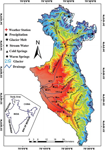
The geology of the catchments is dominated by Upper Palaeozoic and Triassic rocks. The Triassic rocks (carbonates) are surrounded by Palaeozoics (Panjal trap, sandstone and shale, mudstones, slates and phyllites) and are overlain by Pleistocene (Karewa Group) and recent alluvium (Middlemiss 1910, 1911, Wadia 1975). Groundwater discharge occurs through springs, hosted by the Triassic limestone at the contact between the limestone and alluvium (Jeelani 2008). There are two types of karst springs: cold and warm (Jeelani 2004). The water temperatures of cold and warm karst springs are in the ranges 9–14°C and 19–22ºC, respectively. The cold karst springs include Martandnag, Andernag (Liddar catchment), Achabalnag (Bringi catchment) and Daidnag (Kuthar catchment), whereas the warm karst springs include Malakhnag and Gujnag (Kuthar catchment). The discharge is high in cold karst springs (0.3–3 m³ s⁻¹) and low in warm karst springs (0.01–0.09 m³ s⁻¹). Maximum discharge in both cold and warm karst springs occurs during summer and minimum discharge during winter.

3 Methodology

Water samples were collected from precipitation, glacier melt, streams and karst springs in three mountainous catchments in the Western Himalaya: Liddar, Kuthar and Bringi (Fig. 1), for δ²H and tritium (³H) analysis during 2012 and 2013. One year (2013) of available data was used for ³H and two years (2012 and 2013) of data were used for δ²H. For δ²H, the event-based precipitation samples (n = 51) were collected as rain, except in winter when they were as snow, whereas the groundwater samples (n = 70) were collected fortnightly from the karst springs. For ³H, water samples were collected monthly from precipitation (n = 24), streams (n = 21), glacier melt (n = 9) and karst springs (n = 31). The samples from glacier melt were collected during the melting season only (June–November) near the glacier snout. The unfiltered water samples were collected in 10 mL and 500 mL HDPE bottles for δ²H and ³H, respectively. After they had been properly coded and labelled the samples were sent to the Isotope Hydrology Section, Bhabha Atomic Research Centre (BARC), Mumbai, for analysis.

The stable isotope of hydrogen (δ²H) was measured using a dual inlet isotope ratio mass spectrometer (PDZ Europa Geo 2020) by the gas equilibration method. Results for the stable isotopes are reported in the standard δ-notation (Coplen 1996), and are defined in relation to Vienna Standard Mean Ocean Water (VSMOW), as given by the following equation:

(1)

where R_sample represents the isotope ratio of the sample (²H/¹H or ¹⁸O/¹⁶O) and R_standard represents the corresponding ratio of the standard, VSMOW). The δ values are expressed in parts per thousand (per mil, ‰). In order to check the consistency in measurements, samples were analysed in duplicate in each cycle of measurements. Secondary standards used in the batch were pre-calibrated using the primary standards and pre-analysed samples procured from the International Atomic Energy Agency, Vienna (IAEA/WMO 1999). The δ²H values in per mil (‰) are reported relative to VSMOW. The precision of measurement for δ²H is ±0.5‰.

Tritium (³H) analysis was carried out using a liquid scintillation counter (Quantulus Model no. 1220-PerkinElmer) after electrolytic enrichment of samples (Gröning and Rozanski 2004). The tritium values were reported in tritium units (TU). One tritium unit is defined as one atom in 10^–18 atoms of ¹H, which is equivalent to a specific activity of 0.118 bq L⁻¹ of water. The accuracy of the tritium measurement was 0.5 TU. Some previously published data on δ²H (Jeelani et al. 2013) was also used. The MRT was estimated using the tritium method, the sine wave exponential model and tracer experiments.

3.1 Tritium method

The estimation of MRT of the karst groundwater is based on the fact that the tritium input into the groundwater is known, and that of residual tritium measured in the groundwater is the result of decay alone (Clark and Fritz 1997). The MRT was measured according to the following decay equation:

(2)

where a₀ is the initial tritium activity or the concentration in precipitation (input) and a_t is the residual activity concentration in groundwater (output) remaining after decay over time (t). The decay term λ is equal to ln₂ divided by half-life t_1/2. Using the half-life of tritium, t_1/2 = 12.43 years, the equation can be written as (Clark and Fritz 1997):

(3)

and then used in estimating the groundwater age.

3.2 Sine wave model

The monthly and seasonal δ²H values in precipitation and spring water/stream water (input and output signals) were used to estimate MRT of surface/subsurface water using the sine wave exponential model (Bliss 1970, Maloszewski et al. 1983, Burns and McDonnell 1998, Soulsby et al. 2000, McGuire et al. 2002, Rodgers et al. 2005, Jeelani et al. 2013, and others).

The model assumes that the isotopic attenuation reflects the MRT of transport from recharge through the entire flow system and that the recharge is uniformly distributed in time. The model is based on differences between heights of amplitudes of the δ²H variation of precipitation and spring water. Periodic regression analysis (Bliss 1970) was used to fit a seasonal sine wave model to the δ²H time series as:

(4)

where δ²H and X are the predicted and the annual mean measured δ²H, respectively, A is the δ²H annual amplitude (in ‰), c is the radial frequency of annual fluctuations (or 0.017214 rad d⁻¹), t is the time in days after the start of the sampling period, and θ is the phase lag or the time of annual peak δ²H (in radians). Further, Equation (4) can be reformulated using sine and cosine terms in a periodic regression analysis (Bliss 1970) as:

(5)

The estimated regression coefficients β_cos and β_sin are used to compute the amplitude of input and output signal. (√βcos2 +βsin2 were consequently the phase lag tanθ = [βcos /βsin]).

The MRT from the fitted sine wave in the input and output signals is estimated as:

(6)

where Az2 and Az1 are the amplitudes of precipitation and spring water and c is the radial frequency of annual fluctuation defined in the above equation.

3.3 Tracer method

Between August and October 2013, artificial tracer tests were carried out for only three of the major cold karst springs (Achabalnag, Martandnag and Andernag) of the Liddar and Bringi catchments, to estimate the travel time. The tracer tests were not performed for the other springs. A detailed description of the tracer tests is given in Table 1. The first tracer injection was made near Dewalgam village in the Bringi catchment, the second injection was above Mirhai village (near Langnai), Langinalla, in the Liddar catchment and the third at Zajipal, east Liddar. A calibrated portable fluorometer (GGUN-FL30; Albilla Neuchatel, Switzerland) (Schnegg 2002, 2003, Schnegg and Flynn 2002) was set up in each spring before tracer injection and remained on-site until tracer recovery ended. Backup sampling was also carried out every 30 min. The instrument is equipped with four optical components, which are selected according to the absorption–emission spectra of the chosen artificial dye. One of the axes is used to measure the water turbidity using the light source (LED) and other axes are used to measure the fluorescent dye concentrations. Dye concentration (µg L⁻¹) is determined by calibration with solutions of dye at various concentrations. In the present study, Rhodamine WT was used because of its low adsorption on the host rock as compared with other fluorescent dyes (Smart and Laidlaw 1977, Ptak and Strobel 1998).

Table 1. Description of tracer tests performed during 2013.

Location of injection point	Altitude(m a.s.l.)	Distance from spring to injection point (km)	Nature of injection point	Mass injected (kg)	Monitored springs (mean Q during tracer test)
Dewalgam	1940	14	Sink	1	Achabalnag (2.1 m^3 s^−1)
Near Langinai	3500	28	Sinking stream	2	Andernag (0.6 m^3 s^−1)
Zajipal	3500	39	Losing stream	2.5	Martandnag (0.74 m^3 s^−1)

4 Results and discussion

4.1 Variation of tritium in precipitation, glacier melt, streams and karst springs

The tritium values in precipitation ranged from 13.2 to 22.7 TU with an average of 17 TU. The highest tritium values were observed in snow (20.8–22.7 TU) and the lowest in rain (13.2–22.1 TU) with an average of 21.6 and 18 TU, respectively (Fig. 2). High tritium values in snow, i.e. winter precipitation, are attributed to longer transportation of airmass. The low tritium values in rain, the main form of precipitation from March to November in the study area, could be attributed to either local moisture or other sources of airmass from a shorter distance. Spatially, higher tritium values in precipitation were observed at higher elevations (e.g. 3500 m a.m.s.l.: 22.7 TU) and lower ones near the valley floor (e.g. 1600 m a.m.s.l.: 13.2 TU) (Fig. 3). The steadily increasing trend of tritium values with increased altitude could be attributed to atmospheric effects, as the stratosphere is the main reservoir of both natural and bomb-produced tritium (IAEA 1967, Rozanski et al. 1991). At higher elevations, the smaller ground surface to stratosphere distance means higher tritiated water vapour content, which steadily decreases towards lower elevations due to dilution or mixing with lower tritiated air mass (Bradley and Stout 1970). This is supported by the good correlation (R² = 0.83), with corresponding p values (p < 0.008), between average annual tritium values for precipitation collected at various stations and altitudes.

Figure 2. Box and whisker plot showing the minimum, 25th percentile, median, 75th percentile and maximum concentration of tritium in catchment waters.

Figure 3. Relationship between tritium values of individual precipitation samples and altitude.

Temporally, higher tritium values (18.3–22.7 TU) were observed from November to May and lower values (13–17 TU) from June to October (Fig. 4). It is pertinent to mention here that the regional climate of the Western Himalaya is dominated by the Western Disturbances (WDs) originating from the Mediterranean Sea and Indian summer monsoons (ISM) originating from the Bay of Bengal and the Arabian Sea. The WDs cause heavy precipitation (>50% of annual precipitation in winter) in the Western Himalaya from December to May (Pisharoty and Desai 1956, Agnihotri and Singh 1982), while the ISMs bring precipitation from August to October. The higher tritium values from November to May reflect continental sources of air mass and longer transportation of the WDs. The lower tritium values from June to October reflect shorter transport and marine sources of the ISM. The air masses of marine origin have lower tritium input, whereas air masses coming from the continental landmass have higher concentrations of tritium (Rozanski et al. 1991, Ehhalt et al. 2002).

Figure 4. Monthly variation of tritium concentration in precipitation, streams, karst springs and glacier melt for the year 2012/13.

A high tritium value was also observed in one precipitation event in August, which suggested a source of tritium other than the ISM. This high value of tritium in August could be due to (a) vapour left in the atmosphere due to a change in source of air mass after a July rain event; (b) the influence of local moisture with possible effects of moisture recycling by evaporation from local surface water bodies known to enrich the tritium input in precipitation (Warrier et al. 2013); or (c) intense and strong mixing of air masses and re-evaporation of moisture from the continents (Warrier 2010), which also provides higher tritium input in precipitation (Scholz et al. 1970, Ehhalt et al. 2002).

The shift and reversal in the source of air masses during the WD and the ISM is also supported by d-excess of the precipitation. The d-excess values are higher from December to May (16–33‰) than from June to October (–4‰ to 13‰). High average d-excess is attributed to the moisture brought by WDs from the Atlantic Ocean/Mediterranean Sea/Caspian Sea (Jeelani et al. 2013), while the lower d-excess (<15‰) in July, August and September indicates the moisture brought by the ISMs (Kumar et al. 2010). The higher d-excess values (17–28‰, with an average of 22.5‰) of the precipitation event in August may be attributed to the WD as a source of precipitation. As the tritium data of only one precipitation event is available for August, more frequent sampling is required to understand the sources of precipitation.

4.1.1 Glacier melt

The tritium concentration in glacier melt varied in the range 8–12.7 TU, with a mean of 10 TU (Fig. 2). Although glaciers are characterized by low tritium values, the highly variable tritium observed in the glaciers of the study area indicates the addition/mixing of recent precipitation. Generally, the Himalayan glaciers are mixtures of old and new precipitation and even contain recent rain/snow trapped in the glacier. High tritium values in glacier melt were observed in June (12.7 TU) and low ones in August (8 TU) (Fig. 4). The higher tritium values in June/July suggest that the glacial melt collected at the snout is a mixture of winter accumulated recent precipitation and glacier melt. The lower tritium value for August/September is therefore a real representation of the glacier, as the recent snow of the preceding winter was almost completely exhausted by August. It is important to mention here that the glacier samples were taken at the snout as meltwater, which reflects the overall melting behaviour within the catchments of the glacier.

4.1.2 Stream water

Tritium concentration in stream waters varied in the range 11–16.8 TU, with an average of 13.2 TU (Fig. 2). The higher tritium values were observed from March to July (14.5–16.8 TU), when the melting of snow dominantly contributes the streamflow (Jeelani et al. 2013, 2016) and the lower ones from December to February (11–13 TU) (Fig. 4) when the baseflow/groundwater dominantly contributes to the streamflow (Jeelani et al. 2013). This suggests that higher tritium characterized in the snow is reflected in stream water from March to July with a lag of two months. The lower tritium values suggest that baseflow maintains the streamflow during winter, when the contribution from other components, e.g. snow and glacier melt is negligible due to freezing weather conditions. The narrow range of tritium values (13–13.2 TU) in stream water in August–October reflects the combined representation of glacier melt and rain. The tritium values in stream water (i.e. 13–13.2 TU) for this period are much higher than in glacier melt (8–9.2 TU) and lower than for precipitation events (14–22.1 TU). It seems that precipitation events have modified the tritium input of stream water after emerging from the snout. Therefore, the combined role of precipitation and glacier melt cannot be ruled out.

4.1.3 Karst springs

The variation of tritium in karst springs is similar to that of the streams, indicating the dynamic behaviour and quick flushing of water in the karst system. The tritium concentrations in cold and warm karst springs varied in the ranges 11.2–16.5 TU (average: 13.4 TU) and 0.95–9.61 TU (average: 5.3 TU), respectively (Fig. 2). Higher tritium values were observed in cold karst springs and lower ones in warm karst springs. The higher tritium values in cold karst springs reflect the quick response of the recent recharge, whereas the much lower values in the warm karst springs indicate longer circulation and mixing of old and recent recharge. In cold karst springs, the highest tritium values (14.7–16.5 TU) were observed from March to July and the lowest values (11.2–12.5 TU) from August to February (Fig. 4). The high, fickle tritium values indicate recharge from the snowmelt, while the low tritium values in karst springs reflect negligible recharge and discharge from stored water. The low, stable tritium values in August and September (12–12.3 TU) indicate recharge from glacier melt, or from the ISM rainfall. High tritium values in warm karst springs were observed in March–May (9.6 TU), which may be due to the contribution of recent recharge, whereas the lowest values during the remaining months (0.9–3.6 TU) indicate old stored water.

4.2 Mean residence time of karst groundwater

The MRT of groundwater is usually estimated using the tritium method (Rose 2007, Morgenstern et al. 2010), the tritium–helium method (Cook and Solomon 1997, Stolp et al. 2010), chlorofluorocarbons (Plummer and Busenberg 1999, Han 2012), the sulphur hexafluoride method (Busenberg and Plummer 1997, Cook and Herczeg 2000, Gooddy et al. 2006), lumped distribution and sine wave exponential models (McGuire et al. 2002, Tekleab et al. 2014), or artificial tracer experiments (e.g. Spangler 2001, Worthington, 2015). In the present study, we applied the tritium method, sine wave exponential model and tracer experiments to estimate the MRT of groundwater in karst.

4.2.1 Tritium method

This method applies the convolution of a known tritium input via precipitation into the groundwater with an appropriate system response function, and is matched to the measured tritium values in groundwater. The tritium value of the cold karst springs (11.2–16.5 TU) is within the range of present tritium content of the meteoric waters (10–20 TU) in the northern hemisphere (Butler 1955, Rozanski et al. 1991, IAEA 2006). The tritium concentration of groundwater (5–15 TU) is considered to be that of modern groundwater (<5–10 years old), while 0.8–4 TU represents a mixture of sub-modern (prior to 1952) and recent recharge, and <0.8 TU is assumed to be sub-modern recharge (IAEA /WMO 2006, USGS 2006). As the tritium value in the cold karst springs is similar to that in precipitation, the MRT of groundwater in the karst aquifer should be less than 5 years. Lower tritium values in warm springs (0.95–9.61 TU) indicate that the groundwater is a mixture of recent and sub-modern recharge. The lowest tritium value observed in warm springs during winter (0.9 TU) indicates sub-modern recharge, whereas the higher tritium value in summer (9.6 TU) suggests that there is a significant contribution from recent precipitation.

Based on the decay equation (3), the MRT of cold karst springs ranges from 1.5 to 5.1 years, whereas that of warm springs ranges from 5 to 30 years. Among cold karst springs, Achabalnag showed the lowest MRT (1.5–2.6 years), followed by Martandnag (1.8–6 years), Daidnag (2.7–5.1 years) and Andernag (2.8–5 years); in the case of warm karst springs, Gujnag showed a lower age (5–14.8 years) than Malakhnag (14–30 years). The lower MRT of cold springs (Daidnag, Achabalnag, Martandnag and Andernag) can be attributed to rapid circulation and short flow path route with well-developed subsurface drainage. However, the higher MRT of warm springs (Malakhnag and Gujnag) is attributed to a longer circulation route of recharged water and/or mixing of recent precipitation with old stored groundwater.

4.2.2 Sine wave exponential model

The seasonal pattern of δ²H values in precipitation, where winter months are dominated by WDs and summer months by the ISM (as discussed above in Section 4.1), has produced significant seasonal variations (Fig. 5). In comparison to precipitation, δ²H of karst springs, particularly cold karst springs, is also variable (Fig. 6) and exhibits distinctive seasonal variations. However, δ²H is depleted during spring instead of winter as in precipitation and is enriched during summer. It can be observed from δ²H depleted values that there is a lag of 2 months between δ²H of winter precipitation and karst springs (Figs 5 and 6). This type of relationship between the isotopic composition of precipitation and the springs is found in the areas/catchments with snow as the dominant source of stream/spring flow, which not only drains the depleted winter precipitation in late spring, but also minimizes the effect of the enriched stable water isotopic signal of rainfall in summer and autumn. The rise in ambient temperature from March promotes widespread melting of winter precipitation (snow), which generates higher flows during spring and summer in the karst springs and streams of the study region.

Figure 5. Fitted annual regression models for δ²H of precipitation in three catchments for the year 2012/13.

Figure 6. Fitted annual regression models for δ²H of karst springs in three catchments for the year 2012/13.

This temporal/seasonal δ²H pattern observed in precipitation and karst springs was used to estimate MRT using periodic regression analysis. The model described by Equation (4) was used to translate the results into estimates of the MRT according to Equation (6). The calculated results are presented in Table 2. The modelled results suggest that cold karst springs display shorter MRT than warm springs. The MRT of cold karst springs ranged from 2 to 3.4 months; in warm springs it varied from 7 to 9.4 months. Among cold karst springs, Achabalnag and Daidnag showed the lowest MRT (2 and 2.1 months, respectively), followed by Andernag (3.1 months) and Martandnag (3.4 months). However, in the case of warm springs, Malakhnag and Gujnag showed MRT of 7 and 9.4 months, respectively. These δ²H sine wave model results are in agreement with tritium results as they show higher MRT in warm karst springs and lower MRT in cold karst springs.

Table 2. Minimum, maximum and average δ²H values of precipitation of karst springs, with time series correlation (R²) and mean modelled δ²H and amplitude, in the Liddar, Kuthar and Bringi catchments (2012 and 2013).

Location	Min δ^2H	Max δ^2H	Average δ^2H	Amplitude δ^2H	Modelled δ^2H	R^2	MRT (months)
Precipitation
Chandanwari	−73.5	−24.1	−48.12	12.6	−60.75	0.86
Hapatnar	−65.5	−19.7	−43.43	13	−56.48	0.76
Kokernag	−63	−19	−37.27	12.5	−49.77	0.95
Chatrugul	−59.4	−26.7	−47.76	3	−50.75	0.66
Karst springs
Andernag	−54.3	−41.5	−48.77	6.4	−42.37	0.61	3.1
Malakhnag	−54.5	−47.6	−50.83	3.4	−47.41	0.51	7
Gujnag	−54.4	−49.6	−51.87	2.4	−49.40	0.50	9.4
Martandnag	−56.2	−44	−49.96	6.1	−43.86	0.64	3.4
Dauidnag	−54.6	−38	−48.92	8.3	−40.62	0.49	2.1
Achabalnag	−54.3	−37	−48.39	8.6	−39.74	0.76	2

The input signal derived from precipitation alone cannot represent the real input signal to the groundwater in snow and glacierized mountainous catchments (Ofterdinger et al. 2004). The significant contribution of the recharge in these catchments is derived from the melting of snow and ice. Precipitation in winter (December–February) is stored as snow, which enters the flow system in large amounts during the melting season in spring (March–May) and summer (June–August). This time lag in the monitoring input signal from the time of snowfall up to snowmelt, which ranges from a few days (snowmelt commences in March) to about 6 months (most of the snow is exhausted by August), is the primary limitation of this method. Therefore, the MRT estimated using the sine wave model is shorter than that estimated using the tritium method.

4.2.3 Tracer experiments

Groundwater tracing with fluorescent dyes is a useful tool for hydrological investigations in karst terrains (Ford and Williams 2007, Lauber and Goldscheider 2014). During the monitoring period, three dye tests were performed during the high-flow period in 2013 (Table 1). A summary of the results is presented in Table 3. The dye test for Achabalnag, Martandnag and Andernag karst springs was successful and confirmed the hydrological connectivity between the injected tracer locations and the monitored springs. The results of dye tracing indicate that water from losing streams is directed towards the ridge through large joint-controlled rift passages.

Table 3. Summary of results obtained from the tracer experiment.

First arrival time (h)	Peak arrival time (h)	Complete recovery time of tracer mass (h)	Max. conc. (µg L^−1)	Mean flow velocity (m h^−1)	Mass recovered (%)	Longitudinal dispersion (m)
37	49	70	23	254	64	5.4
68	86	130	29	382	52	3.3
77	95	160	21	420	40	8.9

The tracer breakthrough curves (TBC), a primary result of tracer tests, retrieved for different springs (Fig. 7) suggest travel times of groundwater of a few days to a week. Based on the peak arrival of tracer, Achabalnag showed a travel time of >3 days. Similarly, 6–7 days of travel time were determined for Andernag and Martandnag. The variation in the three breakthrough curves reflects the different flow velocities due to different levels of heterogeneity and/or contrast in flow path length as well as differences in hydraulic gradient. Therefore, the retrieved TBCs reveal a high degree of secondary permeability in the host rocks (Triassic limestones) of the study region and indicate a young to mature karst. The quality of the dye test was quantified in terms of mass recovered (Goldscheider et al. 2008). Based on the discharge rate for each spring, the performed tracer experiment gave satisfactory results of 69%, 54% and 40% of injected mass recovered for Achabalnag, Andernag and Martandnag, respectively. Recovery of the injected tracer mass is calculated after Field (2002) and Maqsoud et al. (2007).

Figure 7. Tracer breakthrough curves of three major cold karst springs.

The estimated values of MRT in groundwater using artificial tracers and environmental tracers are supplementary (Worthington 2015). The artificial tracers give the flow velocity and MRT from point source of recharge through sinking streams, swallow holes, sinkholes, etc. to the aquifer outlet and, therefore, represent the short and fast flow route or flow path. However, the environmental tracers give an average age of groundwater recharged through both point source (fast flow) and diffused recharge (slow flow). Therefore, MRT obtained through the injected tracers is always less than that obtained with environmental tracers. Nevertheless, travel time determined through artificial tracer tests provided valuable insight into how quickly changes in discharge and water quality can occur in response to negative changes and/or climatic impact on this vital resource in the region.

4.3 Practical consequences of short travel time: vulnerability

The continuous evaluation of travel/transit times of groundwater in karst terrains is a widely recognized technique to assess vulnerability because travel time is directly related to the diversity of flow paths in a catchment and/or reservoir (Benischke et al. 2007, Perrin et al. 2003, Ford and William 2007). Keeping in view the high permeability, short transit times and multifaceted importance of karst springs in the region (Jeelani et al. 2014), effective approaches are required for the management and protection of karst groundwater resource. Deterioration of quality of water and variation in the magnitude of flux are the two main consequences of the short travel time of karst groundwater in the region. A deterioration of water quality, particularly increases in faecal coliform, faecal streptococci and NO₃, has already been reported (Jeelani 2010). We have observed a rapid change of water colour from transparent to muddy (turbid) soon after every rainfall event in Achabalnag. The identified point source of recharge to the Achabalnag is located close to residential areas and cultivated agricultural fields. There was a significant change in water quality with an increase in NO₃ concentration from 2 to 12 mg L⁻¹ and in Cl from 12 to 31 mg L⁻¹ during summer due to agricultural return flow. Similarly, the point source for the recharge area of Martandnag has been identified near Zajibal along Sheshnag stream. A lot of solid waste and faecal matter is thrown openly to this nalla and this has started to deteriorate the water quality, with an increase in NO₃ concentration to 9 mg L⁻¹. The dependency of karst springs on meltwater (Jeelani 2008, Jeelani et al. 2014), suggests that the change in pattern, form and amount of precipitation due to global warming (Jeelani et al. 2012) might cause considerable variability in spring discharges. There would be a sharp increase in spring flow after each rainfall event and there would be limited perennial recharge if the winter precipitation as snow decreases. This may affect the timing and magnitude of the spring flow. The situation could be worst during the summer season when there is a high demand for water for agricultural and horticultural purposes. The greater variability in precipitation as rain could mean more frequent and prolonged periods of high or low groundwater levels and consequently could affect the flux and storage of water in these aquifers. In 2001, the discharge of the springs was drastically reduced to 40–70% compared to 1999 (Jeelani 2008). In 2013, a significant decrease in discharge was observed in Achabalnag (16%). Other karst springs have also shown significant decreases in discharge (5–10%). The decrease in spring discharge is attributed to below normal precipitation in the preceding winter. The amount of precipitation received during the winter of the monitoring period was 76 mm below normal.

Keeping in view the importance of these karst groundwater resources and their vulnerability, the identified points of recharge and their catchment areas need to be preserved, conserved, managed and protected from anthropogenic activities. Although the protection and mangement of karst aquifers lies within the domain of the government, support from local residents may help to protect and conserve the groundwater in these sensitive and vital karst settings. Knowledge about the importance of these water resources and the recharge catchments needs to be disseminated among the local population, whose livelihood is dependent on these resources.

5 Conclusion

The use of both environmental and artificial tracers (deuterium and tritium) is an adequate way to demonstrate the range of mean residence time (MRT) in karst aquifers. In the present study, the MRT of karst groundwater was estimated in three mountainous catchments of the Western Himalaya, using the tritium method, the sine wave model and artificial tracer tests. The tritium and sine wave modelled results revealed that cold karst springs are recharged with recent recharge, whereas warm karst springs contain a mixture of old and recent recharge. The MRT estimated by the tritium method is comparable with the sine wave model results, with longer MRT in warm karst springs and shorter MRT in cold karst springs. The tracer breakthrough curves (TBC) retrieved for different springs suggested short travel times of groundwater and thus conduit flow. Deterioration of the quality of water and variation in the magnitude of flux are the two main consequences of the short travel time of karst groundwater in the region. Keeping in view the importance of the karst groundwater resource and its vulnerability, the identified point sources of recharge and their catchment areas need to be preserved, conserved, managed and protected from anthropogenic activities.

Acknowledgements

Valuable inputs and suggestions by Jerome Perrin have improved the quality of the manuscript.

Disclosure statement

No potential conflict of interest was reported by the authors.

Additional information

Funding

The research work was funded by the Department of Science and Technology (DST), Government of India, under the research project, DST No: SERB/F/1554/2012.

References

- Agnihotri, S.L. and Singh, M.S., 1982. Satellite study of Western disturbances. Mausum, 33, 249–254.
- Benischke, R., Goldscheider, N., and Smart, C.C., 2007. Tracer techniques. In: N. Goldscheider and D. Drew, eds. Methods in Karst Hydrogeology. London, UK: Taylor & Francis, 147–170.
- Bliss, C.I., 1970. Periodic Regression Statistics in Biology. New York: McGraw- Hill.
- Bradley, W. and Stout, G., 1970. The vertical distribution of tritium in water vapour in the lower troposphere. Urbanu: Illinois State Water Survey, XXII.
- Burns, D.A. and McDonnell, J.J., 1998. Effects of a beaver pond on runoff processes: comparison of two head water catchments. Journal of Hydrology, 205, 248–264. doi:10.1016/S0022-1694(98)00081-X
- Busenberg, E. and Plummer, L.N., 1997. Use of sulfur hexafluoride as a dating tool and as a tracer of igneous and volcanic fluids in ground water. Geological Society of America, 29 (6), A–78.
- Butler, E.B., 1955. Counting tritiated water at high humidities in the Geiger region. Nature, 176, 1262–1264. doi:10.1038/1761262b0
- Clark, I.D. and Fritz, P., 1997. Environmental isotopes in hydrogeology. New York: Lewis Publishers.
- Cook, P.G. and Herczeg, A.L., 2000. Environmental tracers in subsurface hydrology. Boston, MA: Kluwer Academic Publishers.
- Cook, P.G. and Solomon, D.K., 1997. Recent advances in dating groundwater: chlorofluorocarbons, 3H/3He and 85Kr. Journal of Hydrology, 191, 245–265. doi:10.1016/S0022-1694(96)03051-X
- Coplen, T.B., 1996. New guidelines for the reporting of stable hydrogen, carbon and oxygen isotope ratio data. Geochimica Cosmochimica Acta, 60, 3359. doi:10.1016/0016-7037(96)00263-3
- Coward, J.M., Waltham, A.C., and Bowser, R.J., 1972. Karst springs in the valley of Kashmir. Journal of hydrology, 16, 213–223. doi:10.1016/0022-1694(72)90053-4
- DeWalle, D.R., et al. 1997. Seasonal hydrology of three Appalachian forest catchments. Hydrological Processes, 11, 1895–1906.
- Dunn, S.M., McDonnell, J.J., and Vache, K.B., 2007. Factors influencing the residence time of catchment waters: a virtual experiment approach. Water Resources Research, 43. doi:10.6410.01029/02006WR005393
- Ehhalt, D.H., et al., 2002. Tritiated water vapour in the stratosphere: vertical profiles and residence time. Journal Geophysical Research, 107. doi:10.1029/2001JD001343
- Etcheverry, D. and Perrochet, P., 2000. Direct simulation of groundwater transit-time distributions using the reservoir theory. Hydrogeology Journal, 8, 200–208. doi:10.1007/s100400050006
- Field, M.S., 2002. The QTRACER2 Program for tracer-breakthrough curve analysis for tracer tests in karstic aquifers and hydrologic systems. Washington, DC: National Center for Environmental Assessment Washington Office, Office of Research and Development, US Environmental Protection Agency, 20460, EPA/600/R-02/001.
- Ford, D. and Williams, P., 2007. Karst hydrogeology and geomorphology. Chichester: John Wiley and Sons.
- Goldscheider, N., et al., 2008. Tracer tests in karst hydrogeology and speleology. International Journal of Speleology, 37 (1), 27–40. doi:10.5038/1827-806X.37.1.3
- Gooddy, D.C., et al., 2006. Using chlorofluorocarbons (CFCs) and sulphur hexafluoride (SF6) to characterize groundwater movement and residence time in a lowland Chalk catchment. Journal of Hydrology, 330, 44–52. doi:10.1016/j.jhydrol.2006.04.011
- Gröning, M. and Rozanski, K., 2004. Tritium assay in water samples using electrolytic enrichment and liquid scintillation spectrometry. In: En quantifying uncertainty in nuclear analytical measurements. Vienna: IAEA, 195–218. Available from: http://www.iaea.org/programmes/rial/pci/isotopehydrology.
- Han, D.M., 2012. Using chlorofluorocarbons (CFCs) and tritium to improve conceptual model of groundwater flow in the South Coast Aquifers of Laizhou Bay, China. Hydrological Processes, 26 (23), 3614–3629. doi:10.1002/hyp.8450
- Hrachowitz, M., et al., 2013. What can flux tracking teach us about water age distribution patterns and their temporal dynamics? Hydrology and Earth System Sciences, 17, 533–564. doi:10.5194/hess-17-533-2013
- IAEA, 1967. Tritium and other environmental isotopes in hydrological cycle. Technical Report, STI/DOC/10/73, April. Vienna: IAEA.
- IAEA, 2006. Global network of isotopes in precipitation. The GNIP Database. http://www.iaea.org/water
- IAEA/WMO, 1999. Global network of isotopes in precipitation. The GNIP Database. Available from: http://www-naweb.iaea.org/napc/ih/IHS_resources_gnip.html.
- Jeelani, G., 2004. Effect of subsurface lithology on springs of a part of Kashmir Himalaya. Himalayan Geology, 25, 145–151.
- Jeelani, G., 2008. Aquifer response to regional climatic variability in a part of Kashmir Himalaya in India. Hydrogeology Journal, 16, 1625–1633. doi:10.1007/s10040-008-0335-9
- Jeelani, G., 2010. Chemical and microbial contamination of Anantnag springs, Kashmir Valley. Journal of Himalayan Ecology and Sustainable Development, 5, 176–183.
- Jeelani, G., et al., 2012. Role of snow and glacier melt in controlling river hydrology in Liddar watershed (western Himalaya). Water Resources Research, 48, 1–16. doi:10.1029/2011WR011590
- Jeelani, G., et al., 2014. Variation of δ18O, δ2H and 3H in karst springs of south Kashmir, western Himalayas (India). Hydrological Processes, 29 (4), 522–533. doi:10.1002/hyp.10162
- Jeelani, G., et al., 2016. Estimation of snow and glacier melt contribution to Liddar stream in a mountainous catchment, western Himalaya: an isotopic approach. Journal of Isotopes in Environmental and Health Studies. doi:10.1080/10256016.2016.1186671
- Jeelani, G., Kumar, U.S., and Kumar, B., 2013. Variation of δ18O and δ2H in precipitation and stream waters across the Kashmir Himalaya, India, to distinguish and estimate the seasonal sources of streamflow. Journal of Hydrology, 481, 157–165. doi:10.1016/j.jhydrol.2012.12.035
- Jeelani, G. and Shah, R.A., 2016. Delineation of point sources of recharge in karst settings. In: F. Kurisu, et al., eds. Trends in Asian water in Environmental Science and Technology. Cham: Springer International Publishing, Vol. 17, 195–209p.
- Kim, S. and Jung, S., 2014. Estimation of mean water transit time on a steep hillslope in South Korea using soil moisture measurements and deuterium excess. Hydrological Processes, 28, 1844–1857. doi:10.1002/hyp.9722
- Kumar, U.S., et al., 2010. Stable isotope ratios in precipitation and their relationship with meteorological conditions in the Kumaon Himalayas, India. Journal of Hydrology, 391, 1–8. doi:10.1016/j.jhydrol.2010.06.019
- Lauber, U. and Goldscheider, N., 2014. Use of artificial and natural tracers to assess groundwater transit-time distribution and flow systems in a high-alpine karst system (Wetterstein Mountains, Germany). Hydrogeology Journal, 22, 1807–1824. doi:10.1007/s10040-014-1173-6
- Lauber, U., Ufrecht, W., and Goldscheider, N., 2014. Spatially resolved information on karst conduit flow from in-cave dye tracing. Hydrology and Earth System Science, 18, 435–445. doi:10.5194/hess-18-435-2014
- Mahler, B.J. and Massei, N., 2007. Anthropogenic contaminants as tracers in an urbanizing karst aquifer. Journal of Contaminant Hydrology, 91, 81–106. doi:10.1016/j.jconhyd.2006.08.010
- Maloszewski, P., et al., 1983. Application for flow models in an alpine catchment area using tritium and deuterium data. Journal of Hydrology, 66, 319–330. doi:10.1016/0022-1694(83)90193-2
- Maloszewski, P. and Zuber, A., 1982. Determining the turnover time of groundwater systems with the aid of environmental tracers, Models and their applicability. Journal of Hydrology, 57, 207–231. doi:10.1016/0022-1694(82)90147-0
- Maqsoud, A., et al., 2007. Evaluation of hydraulic residence time in the limestone drains of the Lorraine site, Latulippe, Québec. In: Proceedings of the IV International Conference on Mining and the Environment, 19–27 October, Sudbury, Ontario, 1–11.
- McDonnell, J.J., 2010. How old is stream water? Open questions in catchment transit time conceptualization, modelling and analysis. Hydrological Processes, 24, 1745–1754. doi:10.1002/hyp.7796
- McGuire, K.J., DeWalle, D.R., and Gburek, W.J., 2002. Evaluation of mean residence time in subsurface waters using oxygen-18 fluctuations during drought conditions in the mid Appalachians. Journal of Hydrology, 261, 132–149. doi:10.1016/S0022-1694(02)00006-9
- Middlemiss, C.S., 1910. Revision of Silurian-Trias sequence of Kashmir. Record Geological. Survey of India, 40, 206–260.
- Middlemiss, C.S., 1911. Sections in the Pir Panjal range and Sindh Valley, Kashmir. Record Geological Survey of India, 1, 115–144.
- Morgenstern, U., Stewart, M.K., and Stenger, R., 2010. Dating of stream water using tritium in a post nuclear bomb pulse world: continuous variation of mean transit time with streamflow. Hydrology and Earth System Science, 14, 2289–2301. doi:10.5194/hess-14-2289-2010
- Ofterdinger, U.S., et al., 2004. Environmental Isotopes as Indicators for Ground Water Recharge to Fractured Granite. Groundwater, 42 (6), 868–879. doi:10.1111/j.1745-6584.2004.t01-5-.x
- Perrin, J., et al. 2003. Vulnerability assessment in karstic areas: validation by field experiments. Environmental Geology, 46, 237–245.
- Pisharoty, P.R. and Desai, B.N., 1956. Western disturbances and Indian weather. Indian Journal of Meteorology and Geophysics, 8, 333–338.
- Plummer, L.N. and Busenberg, E., 1999. Chlorofluorocarbons. In: P. Cook and A. Herczeg, eds. Environmental tracers in subsurface hydrology. Boston, MA: Kluwer Academic Publishers.
- Ptak, T. and Strobel, H., 1998. Sorption of fluorescent tracers in a physically and chemically heterogeneous aquifer material. In: G.B. Arehart and J.R. Hulston, eds. Water-Rock Interaction. Rotterdam: Balkema, 177–180.
- Rodgers, P., et al., 2005. Using stable isotope tracers to assess hydrological flow paths, residence times and landscape influences in a nested mesoscale catchment. Hydrology and Earth System Sciences, 9, 139–155. doi:10.5194/hess-9-139-2005
- Rose, S., 2007. Utilization of Decadal Tritium Variation for Assessing the Residence time of baseflow. Groundwater, 45, 309–317. doi:10.1111/gwat.2007.45.issue-3
- Rozanski, K., Gonfantini, R., and Araguas–Araguas, L., 1991. Tritium in the global atmosphere: distribution patterns and recent trends. Journal of Physics. Nuclear Part Physics, 17, S523–S536. doi:10.1088/0954-3899/17/S/053
- Schnegg, P.A., 2002. An inexpensive field Fluorometer for hydrogeological tracer tests with three tracers and turbidity measurement. In: E. Bocanegra, D. Marine and H. Massone, eds. Paper presented at the XXXII IAH and VI ALHSUD Congress “Groundwater and Human Development. Argentina: Mar del Plata, 1483-1488.
- Schnegg, P.A., 2003. A new field fluorometer for multi-tracer tests and turbidity measurement applied to hydrogeological problems. In: Paper presented at the 8 Congresso International da Sociedade Brasileira de Geofísica. Rio de Janeiro, RJ: Brazilian Geophysical Society, 14–18.
- Schnegg, P.A. and Flynn, R.M., 2002. Online field fluorometers for hydrogeological tracer tests. In: Isotope und Tracer in der Wasserforschung. Freiberg: Technische Universität Bergakademie, Wissenschaftliche Mitteilungen, Institut für Geologie. Vol. 19, 29–36.
- Scholz, T.G., et al., 1970. Water vapor, molecular hydrogen, methane, and tritium concentrations near the stratopause. Journal of Geophysical Research, 75, 3049–3054. doi:10.1029/JC075i015p03049
- Smart, P.L. and Laidlaw, I.M.S., 1977. An evaluation of some fluorescent dyes for water tracing. Water Resource Research, 13, 15–33. doi:10.1029/WR013i001p00015
- Soulsby, C., et al., 2000. Isotope hydrology of the Allt a’ Mharcaidh catchment, Cairngorm mountains, Scotland: implications for hydrological pathways and water residence times. Hydrological Processes, 14, 747–762. doi:10.1002/(SICI)1099-1085(200003)14:4<747::AID-HYP970>3.0.CO;2-0
- Soulsby, C., et al., 2006. Runoff processes, stream water residence times and controlling landscape characteristics in a mesoscale catchment: an initial evaluation. Journal of Hydrology, 325, 197–221. doi:10.1016/j.jhydrol.2005.10.024
- Spangler, L.E., 2001. Delineation of Recharge Areas for Karst Springs in Logan Canyon, Bear River Range, Northern Utah. U.S. Geological Survey Karst Interest Group Proceedings, Water Resources Investigations Report, 01-4011, 186–193.
- Stewart, M.K., et al., 2012. The ‘hidden streamflow’ challenge in catchment hydrology: a call to action for stream water transit time analysis. Hydrological Processes, 26, 2061–2066. doi:10.1002/hyp.9262
- Stolp, B.J., et al., 2010. Age dating baseflow at springs and gaining streams using helium-3 and tritium: Fischa-Dagintz system, southern Vienna Basin, Austria. Water Resources Research, 46, W07503. doi:10.1029/2009WR008006
- Tekleab, S., Wenninger, J., and Uhlenbrook, S., 2014. Characterisation of stable isotopes to identify residence times and runoff components in two mesoscale catchments in the Abay/Upper Blue Nile basin, Ethiopia. Hydrology Earth System Sciences, 18, 2415–2431. doi:10.5194/hess-18-2415-2014
- USGS, 2006. The Reston Chlorofluorocarbon Laboratory: 3H/3He dating background. Available from: http://water.usgs.gov/lab/3h3he/background/, 6 p
- Wadia, D.N., 1975. Geology of India. New Delhi: Tata McGraw Hill.
- Warrier, C.U., 2010. Isotopic characterization of dual monsoon precipitation- evidence from Kerala, India. Current Science, 98 (11), 1487–1495.
- Warrier, C.U., et al. 2013. Spatial and temporal variations of natural tritium in precipitation of southern, India. Current Science, 105, 25–242.
- Worthington, S.R.H., 2007. Groundwater residence times in unconfined carbonate aquifers. Journal of Caves and Karst Studies, 69, 94–102.
- Worthington, S.R.H., 2015. Diagnostic tests for conceptualising transport in beed rock aquifers. Journal of Hydrology, 529, 365–372. doi:10.1016/j.jhydrol.2015.08.002