Long-term analysis of measured and simulated evapotranspiration and soil water content

ABSTRACT

In our study, we analysed a period from 2003 to 2012 with micrometeorological data measured at a boundary-layer field site operated by the Lindenberg Meteorological Observatory – Richard-Aßmann-Observatory of the German Meteorological Service (DWD). Amongst others, these data consist of real evapotranspiration (ETr) rates measured by eddy covariance and soil water contents determined by time domain reflectometry. Measured ETr and soil water contents were compared with those simulated by a simple soil–vegetation–atmosphere transfer (SVAT) scheme consisting of the FAO56 Penman-Monteith equation and the soil water flux model Hydrus-1D. We applied this SVAT scheme using uncompensatory and compensatory root water uptake (RWU). Soil water contents and ETr rates calculated using uncompensatory RWU showed an acceptable fit to the measured ones. In comparison, the use of compensatory RWU resulted in lower model performance due to higher deviations between measured and simulated soil moisture values and ETr rates during dry summer periods.

KEYWORDS:

• modelling
• real evapotranspiration
• soil water content
• eddy covariance
• compensatory root water uptake model

Editor A. Castellarin Associate editor N. Verhoest

1 Introduction

Real evapotranspiration (ETr) is an important part of the water balance equation (e.g. Katul et al. 2012). Therefore, much work has been carried out to improve methods for the measurement and calculation of ETr (e.g. Allen et al. 2011).

Nowadays, in situ measurements of ETr are carried out using weighable lysimeters, the soil water budget method, the Bowen ratio method, scintillometers, and the eddy covariance (EC) method (e.g. Allen et al. 2011, Evett et al. 2012a). Among all these techniques, the EC method is currently considered to be the most appropriate technique for a precise determination of ETr at field scale (e.g. Allen et al. 2011, Evett et al. 2012a).

For a physically-based calculation of ETr, the application of computer codes using the Penman-Monteith equation for the estimation of evapotranspiration and numerical models for the calculation of root water uptake (RWU), soil evaporation and soil water fluxes has been established (e.g. Kool et al. 2014, Soylu et al. 2014, Pereira et al. 2015). Within such soil water flux models, the spatial distribution of RWU over the root zone depending on rooting depth and root density distribution in the soil profile is calculated using various RWU models. A current overview of such RWU models is given in, for example, Kumar et al. (2015). Over the past decade, physically-based compensatory RWU models for improved calculation of soil water uptake by plant roots have been developed (e.g. Yadav et al. 2009, Jarvis 2011, de Willigen et al. 2012, Vogel et al. 2013, Albasha et al. 2015). Such RWU models enable the compensation of reduced RWU in upper dry soil layers by an increased uptake in deeper wetter soil layers.

Studies on the testing of such compensatory RWU models using experimental field data with in situ measured ETr rates and soil water contents have been published in Braud et al. (2005), Yadav et al. (2009), Dong et al. (2010), Deb et al. (2011), Shouse et al. (2011) and Deb et al. (2013), among others. In these studies, the experimental field data covered periods of up to 3 years and the application of compensatory RWU models resulted in improved predictions for soil water content and RWU whilst corresponding predictions obtained from uncompensatory RWU models were less accurate than those using compensation (e.g. Jarvis 2011, de Willigen et al. 2012). In contrast, in new simulation studies published by dos Santos et al. (2016) and Peters (2016), for example, some conceptual shortcomings of the compensatory RWU models applied in studies such as Jarvis (2011) and de Willigen et al. 2012 were reported. The most important shortcoming was an unnatural abrupt decrease of RWU under dry conditions (dos Santos et al. 2016, Peters 2016). However, the results of these new simulation studies were not validated with corresponding experimental field data until now. Therefore, the need for a further thorough validation of such compensatory RWU models using longer time series of measured ETr rates and observed soil hydrological conditions was emphasized.

In a previously published paper (Wegehenkel and Beyrich 2014), hourly ETr rates measured by the EC method and soil water contents measured by time domain reflectometry (TDR) probes at a boundary-layer field site for a period from 2003 to 2004 were compared with those calculated by a numerical soil–vegetation–atmosphere transfer (SVAT) modelling approach using an uncompensatory and a compensatory RWU model. In comparison with the uncompensatory approach, the use of the compensatory RWU model resulted in a lower goodness of fit between measured and simulated ETr and soil water contents. These results were in contrast to those published in the previously mentioned studies of the application of compensatory RWU (e.g. Jarvis 2011, de Willigen et al. 2012). In the year 2003, extreme warm and dry weather conditions led to the hottest summer on record in Europe since 1540 (e.g. García-Herrera et al. 2010). Therefore, and due to the short time period of only 2 years, these findings were considered as preliminary and should be substantiated by a further long-term analysis (Wegehenkel and Beyrich 2014).

Therefore, the main objectives of our study were

• a further long-term analysis of the impact of the use of uncompensated and compensated RWU with different parametrizations on simulated ETr, soil water contents, soil water fluxes and on the model performance.

• a more detailed insight into the long-term behaviour of the compensatory RWU model under varying meteorological and soil hydrological boundary conditions.

• an analysis of the limitations and shortcomings of compensatory RWU models using long-term experimental field data.

For that purpose, we now analyse a 10-year period from 2003 to 2012 with hourly ETr rates and soil water contents observed at the same boundary-layer field site. As far as the authors know, this is one of the first studies on model validation using such a time series of 10 years with an hourly time step.

2 Material and methods

2.1 Falkenberg field site

The micrometeorological field data measured at the grass-covered Falkenberg boundary-layer field site covered the time period from 1 January 2003 to 31 December 2012. These observations were carried out by the Lindenberg Meteorological Observatory – Richard-Aßmann-Observatory, which is part of the German Meteorological Service (Deutscher Wetterdienst, DWD). This observatory is located in northeast Germany about 60 km southeast of Berlin and the boundary-layer field site is located 5 km south of the observatory. The terrain around the Falkenberg test site is slightly sloping from NNE towards SSW with height differences of less than 5 m over a distance of about 1 km. The central part of the boundary-layer field site is a flat meadow of 150 m × 250 m covered by short grass. Thus, the surface at the Falkenberg field site can be classified as homogeneous (Beyrich et al. 2006). The observed micrometeorological field data (see Table 1) consist of:

• Precipitation, net radiation, air temperature, air humidity and wind speed data.

• Determination of momentum, sensible and latent heat fluxes by eddy covariance (EC) systems.

• Monitoring of soil water contents, soil temperatures and soil heat flux.

Table 1. Measurements at the Falkenberg boundary-layer field site (from Wegehenkel and Beyrich 2014, modified).

Measurement system	Measured parameter	Sensor/ Manufacturer	Measurement height (+) or depth (−) (m)
10 m tower	Temperature (°C), rel. air humidity (%)	HMP-45/Vaisala	0.5, 1, 2, 4, 10
	Wind speed (m s^−1)	F460/Climatronics	0.25, 0.5, 1, 2, 4, 6, 8, 10
	Wind direction (deg)	Wind direction transmitter/Thies/Young (since 2008)	11/11.5
	Air pressure (hPa)	PTB 220 A/Vaisala	1
	Precipitation (mm)	Pluvio/Ott	1
	Shortwave radiation (W m^−2)	CM14/CM24 (since 2006) Kipp & Zonen	2
	Longwave radiation (W m^−2)	DDPIR/Eppley	2
Turbulence measurements	Momentum, sensible and latent heat fluxes (W m^−2)	USA-1 sonic/METEK) LI-7500 infrared hygrometer/LiCor	2.4
Soil measurement place	Soil water content	TRIME-EZ/IT Imko	−0.08, −0.15, −0.30,
			−0.45, −0.60, −0.90
	Soil temperature	Pt-100/TMG	−0.05, −0.10, −0.20,
			−0.30, −0.45, −0.50,
			−0.60, −0.90, −1.00,
			−1.50
	Soil heat flux	HP3/RIMCO	−0.05, −0.10

The soil at the test site was formed by the inland glaciers of the last ice age, and the corresponding basic soil physical properties are summarized in Table 2. More details can be found in Beyrich and Mengelkamp (2006), Beyrich et al. (2006) and Beyrich and Adam (2007).

Table 2. Soil physical properties at the Falkenberg field site (from Wegehenkel and Beyrich 2014) (Eutric Podzoluvisol (FAO, 1988)).

Horizon	Depth (cm)	Sand (%) (2.0–0.063 mm)	Silt (%) (0.063–0.002 mm)	Clay (%) (<0.002 mm)	Bulk density (g cm^−3)
Ap	0–30	70	25	5	1.6
Ael	30–60	70	26	4	1.7
Bv	>60	55	25	20	1.7

Eddy covariance measurements were carried out using two EC stations positioned at the eastern (E) and western (W) sides of the meadow. The W station has an undisturbed fetch sector between 030° and 180°, and the fetch sector of the E station ranges between 150° and 330°. A composite flux dataset was created from the measurements for these two stations, ensuring that the measured signals basically originate from the grassland area and are independent of the wind direction. Footprint calculations for both stations were performed for a set of wind direction and stability sectors as described in Mauder et al. (2006). These calculations indicated that more than 95% of the flux footprint is covered by the grassland surface under unstable conditions (the more relevant regime with respect to turbulent exchange), for stable conditions more than 67% of the flux footprint is covered by the meadow. The EC measurements were carried out at a 20-Hz sampling rate, the fluxes were calculated using double rotation of the coordinate system, and corrections for spectral losses, cross wind, buoyancy and density effects (e.g. Mauder et al. 2006, Beyrich and Adam 2007). For our study, all measured field data were aggregated to hourly values. An assessment of the measurement accuracy of the EC stations for hourly ETr in the study of Mauder et al. (2006) yielded a mean error ≤ 30 W m⁻² ≈ 0.04 mm h⁻¹. The EC data showed gaps in the time series of hourly sensible (about 1% of the values) and latent (about 17% of the values) heat fluxes (Table 3). These gaps were not filled. This higher amount of missing values for the latent heat flux is mainly due to wet sensor windows of the infrared hygrometer during periods of rain, fog or dew formation. Under such conditions, the absolute flux values can be assumed small.

Table 3. Numbers of simulated and measured hourly ETr rates per year.

Year	Number of simulated ETr rates per year	Number of measured ETr rates per year	Missing measured ETR rates as percentage of number of simulated ETr rates
2003	8760	6837	22
2004	8784	7559	14
2005	8760	7569	14
2006	8760	7247	17
2007	8760	7583	13
2008	8784	7070	20
2009	8760	7350	16
2010	8760	6947	21
2011	8760	7066	19
2012	8784	7275	17

Time domain reflectometry (TDR) probes were installed horizontally at six depths (Table 1) for measuring soil water content. In the upper part of the soil profile, four TDR probes were installed at 8 cm, and three probes at 15 cm depth in order to determine the spatial variability caused mainly by small-scale heterogeneity of the vegetation cover. For these two depths, we used the mean values of the measurements of the four or three TDR probes as the final measured soil water contents. The corresponding standard deviations were below 0.02 cm³ cm⁻³. The soil water contents below 15 cm were measured by a single probe at each depth. The TDR probes were used with the manufacturer’s calibration, which is valid for sandy soil. Calibration for all probes was checked before installation according to the procedures recommended by the manufacturer using a mixture of water and glass beads in a well-defined ratio. The precision of the TDR probes installed in the field was assessed by periodical comparison with field gravimetry sampled at varying distances (10–400 m) from the location of the TDR probes. These comparisons showed a mean deviation between soil water contents measured by TDR and those determined by gravimetry of 0.02–0.05 cm³ cm⁻³ in the soil layers above 45 cm depth. In the soil layers below 45 cm depth, deviations from 0.05 cm³ cm⁻³ and in some cases up to 0.15 cm³ cm⁻³ were found. These larger deviations were attributed to the high spatial heterogeneity of the depth location of the Bv soil horizon in the soil profile at the Falkenberg field site. This soil horizon located at the lower boundary of the soil profile has a significantly higher clay content than the two upper soil horizons (Table 2). Therefore, this spatial variation of the depth location of the Bv horizon led to a spatially highly variable content of sand and clay between about 40 and 90 cm depth (Beyrich and Mengelkamp 2006). Such spatial variations in soil texture can lead to larger deviations between soil water contents measured by TDR probes and those determined by field gravimetry (e.g. Bitteli et al. 2008). In other studies, deviations between TDR and field gravimetry ranged from 0.01 up to 0.09 cm³ cm⁻³ (e.g. Bitteli et al. 2008, Robinson et al. 2008, Evett et al. 2012b). The deviations between soil water contents measured by TDR and those determined by gravimetry at the Falkenberg site were in the same range. More details about the soil hydrological measurements can be obtained from Beyrich and Adam (2007), for example.

2.2 Simulation models

In the recent study, we used a model chain consisting of a physiologically-based grass-cover growth model and the numerical soil water flux model Hydrus-1D.

2.2.1 Model for grass-cover growth

Here, grass-cover growth is calculated using algorithms according to the Wofost6.0 model (Supit et al. 1994). The model simulates time series of crop parameters such as daily above-ground biomass and leaf area index, LAI. Growth of grass cover is limited by soil water availability for root water uptake and air temperature stress. The calculation of mowing dates is based on user-defined threshold values of above ground biomass. At these threshold values, it is assumed that grass is being mowed and harvested. More details can be found in Wegehenkel and Gerke (2013), for example, and in Wegehenkel and Beyrich (2014). This model was applied to calculate the time series of LAI needed as one input for the model runs of Hydrus-1D (Simunek et al. 2013).

2.2.2. Hydrus-1D

Saturated–unsaturated soil water fluxes are calculated by a numerical solution of the Richards’ equation:

(1)

where θ is the volumetric soil water content in cm³ cm⁻³, t is time, z is depth, and h is the water pressure head, both in cm. K(h) is unsaturated hydraulic conductivity (cm T⁻¹). The time unit T for the model runs can range from days, hours, minutes to seconds (Simunek et al. 2013). S is the sink term (T⁻¹) for the estimation of root water uptake (RWU) according to Feddes et al. (1978):

(2)

T_pot is the potential RWU rate in cm T⁻¹, ß(z) is the normalized root density function used for the vertical distribution of T_pot over the root zone, and a(h) is a dimensionless function (0 ≤ a ≤ 1) of actual water pressure head h (cm) used to calculate the impact of water stress on T_pot. For a(h), we used the function of Feddes et al. (1978) with the threshold parameters h₄, h₃, h₂ and h₁ (cm). The actual uncompensated RWU rate T_a in cm T⁻¹ is given by:

(3)

Here, Lr is depth of the root zone in cm. The compensatory RWU model uses a weighted stress index ω in the range 0 < ω < 1:

(4)

A value of ω = 1 means no stress conditions in the root zone. The actual compensated RWU rate T_ac is defined as:

(5)

where ω_c is the critical RWU index (0 < ω_c < 1). The compensated RWU rate T_ac is equal to T_pot when ω > ω_c. In the case of ω < ω_c, RWU is increased uniformly throughout the root zone by a compensatory factor 1/ω to keep T_ac equal to T_pot. More information about RWU compensation can be found in Jarvis (2011).

In our study, the soil surface boundary was defined by an atmospheric boundary condition determined by rainfall or by evaporation.

Simulation of snow accumulation and snow melting was based on the calculation of heat transfer using a convection–dispersion equation. Snow accumulation was calculated at air temperatures below −2°C. Snow melting occurs at air temperatures above zero and an existing snow layer melts proportionally to the air temperature using a snow melting constant. More information can be obtained from Simunek et al. (2013).

For the soil water flux calculations according to Equation (1), we used the hydraulic conductivity function K(h) according to Mualem (1976) and the soil water retention function θ(h) from van Genuchten (1980):

(6)

where K(h) is the unsaturated hydraulic conductivity in cm T⁻¹ at the actual pressure head h in cm; K_sat is the saturated hydraulic conductivity in cm T⁻¹; α in cm⁻¹ and n without dimensions are soil texture-specific parameters with the threshold m = 1–1/n; θ is the actual soil water content; θ_s and θ_r are saturated and residual soil water contents, all in cm³ cm⁻³.

The numerical solution of Equation (1) is based on the use of Galerkin-type linear finite element schemes. Integration in time is achieved using an implicit (backwards) finite difference scheme (Simunek et al. 2013).

2.3 Model set-up

2.3.1 Model for grass-cover growth

The inputs for this model were daily rainfall, global radiation, wind speed, temperature and air humidity calculated from the hourly data measured at the Falkenberg field site. The simulation of parameters such as daily LAI covered the overall investigation period from 1 January 2003 to 31 December 2012. The maximum rooting depth of the grass cover was set at 50 cm according to corresponding literature data (Supit et al. 1994), and the threshold value of above ground biomass for the simulation of mowing dates was set at 2400 kg ha⁻¹ (Wegehenkel and Beyrich 2014).

2.3.2 Hydrus-1D

Due to the hourly modelling time step according to the time resolution of the measured micrometeorological data, hourly values of LAI had to be estimated using linear interpolation between two adjacent calculated daily values of LAI (Wegehenkel and Beyrich 2014). Thus, hourly rates of measured precipitation and of calculated potential grass reference evapotranspiration (ETp), and hourly values of LAI were used as input for the model runs of Hydrus-1D for the time period from 2003 to 2012. This period corresponds to a total of 87 670 hours. For the calculation of soil water fluxes, the 150-cm-deep soil profile was discretized into 150 nodes, each with 1 cm thickness.

Heat transport, snow cover accumulation and snow melt were simulated using measured soil temperatures at 5 cm depth as upper and at 150 cm depth as lower boundary conditions. The snow melting constant was set at 0.43 cm. The soil thermal conductivity λ(θ) (MLT⁻³ K⁻¹) was calculated using the Chung and Horton approach (Chung and Horton 1987):

(7)

For the empirical parameters b₁, b₂, b₃, we used the default values: b₁ = 0.228, b₂ = −2.406 and b₃ = 4.909 W m⁻¹ K⁻¹ for the two upper sandy horizons of the soil profile (Table 2), and b₁ = 0.243, b₂ = 0.393 and b₃ = 1.534 W m⁻¹ K⁻¹ for the lower loamy soil horizon according to Chung and Horton (1987).

Hourly rates of ETp in mm h⁻¹ were calculated using the FAO56-Penman-Monteith equation (Allen et al. 1998):

(8)

where Δ is the slope of the saturation vapour pressure curve at T_hour in kPa °C ⁻¹; Rn is the net radiation at the grass surface and G is the soil heat flux density, both in MJ m⁻² h⁻¹; γ is the psychrometric constant in kPa °C ⁻¹; T_hour is the mean air temperature (°C); U₂ is the average wind speed at 2 m height in m s⁻¹; e^s_hour (T_hour) is the saturation vapour pressure at T_hour and e_a is the actual vapour pressure, both in kPa.

Net radiation, soil heat flux and latent heat flux were measured as energy flux densities in W m² (Table 1). Therefore, net radiation and soil heat flux had to be converted to MJ m⁻² for the calculation of ETp, and latent heat flux was converted to the hourly evapotranspiration equivalent ETr in mm h⁻¹:

(9)

where LE is the latent heat flux (W m⁻²), ρ_ω is the water density (kg m⁻³), L_v is the latent heat of vaporization (J kg⁻¹), and T_air is the air temperature (°C).

The separation of hourly ETp in potential soil evaporation E_pot and potential RWU T_pot is calculated using interpolated hourly LAI:

(10)

where ext_coeff is an extinction coefficient of radiation (Ritchie 1972). In our study, we used a value of ext_coeff = 0.6 for grass cover (Supit et al. 1994). The reduction of E_pot to real evaporation e_real and of T_pot to actual RWU T_a is calculated by Hydrus-1D depending on available soil water for evapotranspiration. Simulated real evapotranspiration ETr is then defined as the sum of e_real and T_a.

The lower boundary condition for the soil water flux calculations was free drainage. The van Genuchten-Mualem parameters θ_s, θ_r, α, n and saturated hydraulic conductivity K_sat (Table 4) were obtained from the former study (Wegehenkel and Beyrich 2014). The soil water contents at field capacity (i.e. pF (log (height of water in cm)) = 1.8, h = 63 cm) calculated from the water retention functions in Table 4 were used as initial condition for the model calculations.

Table 4. Van Genuchten-Mualem parameters (see Equation (6)) for the Falkenberg field site (from Wegehenkel and Beyrich 2014).

Horizon	θs (cm^3 cm^−3)	θr (cm^3 cm^−3)	α (cm^−1)	n	Ksat (cm h^−1)
Ap	0.37	0.00	0.0238	1.3825	1.6
Ael	0.35	0.08	0.0259	1.2759	0.6
Bv	0.45	0.21	0.0303	1.1624	0.4

For the simulation of uncompensatory and compensatory RWU, we used the same maximum rooting depth of grass cover at 50 cm as for the grass-cover growth model, the assumption of a linear decrease of ß(z) in Equation (2) with soil depth and the threshold values h₁, h₂, h₃ and h₄ for grass cover according to an internal Hydrus-1D database (Simunek et al. 2013).

The critical RWU stress index ω_c in Equation (5) required for the application of RWU compensation is an empirical constant depending on root length density, potential RWU, soil texture and above-ground plant properties (e.g. Jarvis 2011). Currently, little information exists in literature about the values of the ω_c threshold. In a study by Shouse et al. (2011), this threshold was set empirically to ω_c = 0.25. In other studies, such as those published by Deb et al. (2011) and by Albasha et al. (2015), ω_c was in a range from 0.5 to 1.0. Therefore, we decided to use three different values of ω_c, namely with 0.25, 0.50 and 0.75. A similar range of ω_c values was applied in the modelling study of Peters (2016).

2.3.3 Estimation of the goodness of fit between model outputs and measurements

For the estimation, we used the Nash-Sutcliffe index NS (Nash and Sutcliffe 1970), modelling efficiency index IA (Willmott 1982), coefficient of determination R² and the root mean squared difference RMSD.

(11a)

(11b)

(11c)

(11d)

where θ_sim and θ_obs are simulated and observed values; n is the number of data pairs, and θ_obs-mean and θ_sim-mean are the corresponding mean values. The NS index ranges between −∞ and 1, IA and R² are in the range from 0 to 1. A value of 1 suggests a perfect fit of simulated to observed values.

3 Results and discussion

3.1 Grass-cover growth model

The input data for the model runs of Hydrus-1D consist of hourly measured precipitation, air and soil temperatures, simulated ETp and hourly LAI (Fig. 1).

Figure 1. Measured hourly rainfall, simulated snow accumulation (Snow), observed hourly air temperatures at 2 m height (T_air), measured and simulated soil temperatures at depths of 10 and 150 cm (T_10cm, T_150cm), calculated hourly leaf area index (LAI) and potential grass reference evapotranspiration (ETp) for Falkenberg, 2003–2012.

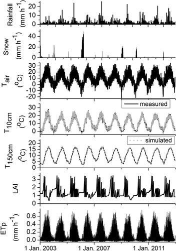
Comparison of simulated with actual mowing dates in the previous publication indicated an adequate calculation of the time series of LAI at the Falkenberg field site (Wegehenkel and Beyrich 2014).

3.2 Hydrus-1D

3.2.1 Simulated and measured time series of soil temperatures and soil water contents

The long-term mean annual precipitation at the Lindenberg observatory located near the Falkenberg test site for the period from 1907 to 2010 is at 556 mm. Annual precipitation rates from 2003 to 2012 observed at the field site ranged from 353 to 733 mm, thus indicating the occurrence of both dry and wet years during the investigation period (Table 5).

Table 5. Precipitation totals at the Falkenberg field site.

Year	Annual precipitation (mm)	Hydrological summer half-year (May–October) (mm)
2003	375	207
2004	498	277
2005	546	386
2006	353	189
2007	638	398
2008	560	249
2009	534	327
2010	733	482
2011	555	398
2012	590	355

Simulated and measured hourly soil temperatures showed only minor differences (Fig. 1), and the match between simulated and measured soil temperatures was described by an IA of 1.00, NS of 0.99 and RMSD of 0.4°C for all depths from 5 cm down to 150 cm. In other studies, the goodness of fit between calculated and observed soil temperatures in terms of IA (0.95–0.96) and of RMSD (1.5–4.8°C) was lower (e.g. Deb et al. 2011, Sándor and Fodor 2012).

In our figures, we focus on two selected periods, one from 2003 to 2006 (Figs 2 and 4(a)), and one from 2007 to 2010 (Figs 3 and 4(b)). The years 2003 and 2006 showed the lowest annual rainfall rates of 375 and 353 mm, which ranged significantly below the long-term mean annual rate. In addition, the lowest rainfall sums for the hydrological summer half-years from May to October, at 207 and 189 mm, must have been observed in these two years (Table 5). The years 2007 with 638 mm and 2010 with 733 mm showed the highest annual precipitation sums during this 10-year period, significantly higher than the long-term mean annual sum. For the corresponding hydrological summer half-years, precipitation of 398 mm was observed in 2007 and rainfall of 482 mm was measured in 2010 (Table 5).

Figure 2. Hourly rates of rainfall and real evapotranspiration (ETr) measured by the EC system (EC), hourly soil water contents in the topsoil layer (1 cm) and at 8, 15 and 30 cm depth measured by TDR in comparison with those simulated using a rooting depth of 50 cm, uncompensated (uncompensated-50cm) and compensated RWU with ω_c = 0.25 (compensated-50cm ω_c = 0.25) and by using a rooting depth of 100 cm (uncompensated-100cm) for Falkenberg, 2003–2006.

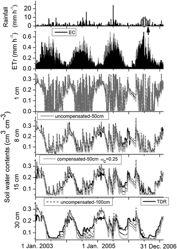
Figure 3. Hourly rates of rainfall and real evapotranspiration (ETr) measured by the EC system (EC), hourly soil water contents in the topsoil layer (1 cm) and at 8, 15 and 30 cm depth measured by TDR in comparison with those simulated by using a rooting depth of 50 cm, uncompensated (uncompensated-50cm) and compensated RWU with ω_c = 0.25 (compensated-50cm ω_c = 0.25) and using a rooting depth of 100 cm (uncompensated-100cm) for Falkenberg, 2007–2010.

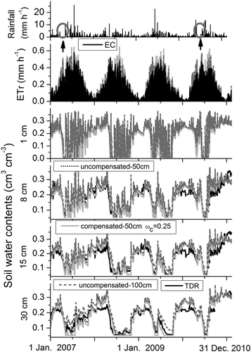
Figure 4. Observed hourly rainfall and hourly soil water contents at 45, 60 and 90 cm depth measured by TDR in comparison with those simulated using a rooting depth of 50 cm, uncompensated (uncompensated-50cm) and compensated RWU with ω_c = 0.25 (compensated-50cm ω_c = 0.25) and using a rooting depth of 100 cm (uncompensated-100cm) for Falkenberg: (a) 2003–2006, (b) 2007–2010.

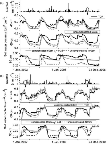
Between January and March in 2003 and 2006, measured soil temperatures from 5 cm down to 30 cm depth indicated frozen soil conditions due to air temperatures down to −15°C and simulated snow cover accumulation in January–March 2006 resulted in more or less constant simulated soil water contents down to 30 cm depth (Figs 1 and 2). These frozen soil conditions also led to an abrupt decrease of measured soil water contents because TDR probes detect only liquid water. Therefore, these periods with frozen soil conditions in the time series of observed soil water contents were excluded from our analysis. In both dry years, 2003 and 2006, simulated and measured soil water contents in the summer periods were low and often near or at the wilting point (Figs 2 and 4(a)). Compared to that, the two wet years, 2007 and 2010, showed only short periods with low soil water contents (Figs 3 and 4(b)).

Measured soil water contents at 8, 15 and 30 cm depth and those simulated by using a rooting depth of 50 cm, and uncompensatory and compensatory RWU run similarly (Figs 2 and 3). Therefore, the goodness of fit between simulated and measured soil water contents was described by values of IA from 0.91 to 0.96, NS between 0.51 and 0.83, and RMSD within 0.03–0.04 cm³ cm⁻³, thus indicating an adequate simulation of RWU and soil water fluxes in this part of the root zone (Table 6). In contrast to that, simulated soil water contents at 45 cm depth in the winter and spring periods from 2003 to 2006 were sometimes higher than the measured ones, whereas calculated soil water contents at 60 cm depth in the summer periods were distinctly lower than the observed ones (Fig. 4(a)). This indicates an overestimation of RWU at 60 cm depth by our modelling approach (Fig. 4(a)). In the second period, from 2007 to 2010, simulated and measured soil water contents at 45 and 60 cm depths showed a better match (Fig. 4(b)). Therefore, measurement errors of the TDR-probes as a reason for this mismatch between simulated and measured soil water contents in the first period from 2003 to 2006 seems unlikely (Fig. 4). Due to this mismatch, the goodness of fit between simulated and measured soil water contents at 45 and 60 cm depths was described by lower values of IA from 0.69 to 0.88 and NS between −1.2 and 0.48 (Table 6). Measured soil water contents at 90 cm depth in the summer periods of 2003 and 2006 and from 2008 to 2010 were lower than those simulated using a rooting depth of 50 cm, and compensatory and uncompensatory RWU (Fig. 4). This indicates an underestimation of RWU in this part of the root zone by our modelling approach for these years. Thus, the model performance was poor, mainly suggested by an IA of 0.54–0.56 (Table 6).

Table 6. Modelling efficiency index IA, Nash-Sutcliffe index NS, coefficient of determination R² and root mean squared difference RMSD for soil water contents calculated with different model configurations using the 10-year dataset (2003–2012) from the Falkenberg field site.

Depth	IA	NS	R^2	RMSD (cm^3 cm^−3)
Rooting depth 50/100 cm
(a) Uncompensated root water uptake
8 cm	0.96/0.96	0.83/0.84	0.85/0.87	0.03/0.03
15 cm	0.95/0.94	0.80/0.74	0.85/0.85	0.03/0.03
30 cm	0.93/0.92	0.66/0.62	0.80/0.77	0.04/0.04
45 cm	0.88/0.89	0.48/0.49	0.62/0.57	0.04/0.04
60 cm	0.77/0.76	−0.32/−0.7	0.59/0.67	0.03/0.06
90 cm	0.56/0.69	0.24/−0.16	0.34/0.34	0.03/0.04
(b) Compensated root water uptake ωc = 0.75
8 cm	0.95/0.96	0.81/0.83	0.84/0.85	0.03/0.03
15 cm	0.95/0.96	0.78/0.80	0.84/0.85	0.03/0.03
30 cm	0.92/0.92	0.59/0.62	0.79/0.80	0.04/0.04
45 cm	0.87/0.80	0.41/-0.29	0.59/0.61	0.04/0.06
60 cm	0.73/0.54	−0.67/−4.98	0.55/0.51	0.06/0.11
90 cm	0.55/0.59	0.24/0.24	0.32/0.24	0.03/0.03
(c) Compensated root water uptake ωc = 0.50
8 cm	0.95/0.96	0.79/0.82	0.85/0.85	0.03/0.03
15 cm	0.95/0.95	0.76/0.80	0.84/0.85	0.03/0.03
30 cm	0.91/0.91	0.54/0.56	0.78/0.77	0.04/0.04
45 cm	0.86/0.77	0.34/−0.56	0.59/0.57	0.04/0.06
60 cm	0.71/0.54	−0.87/−5.70	0.54/0.51	0.06/0.11
90 cm	0.55/0.59	0.24/0.23	0.31/0.24	0.03/0.03
(d) Compensated root water uptake ωc = 0.25
8 cm	0.95/0.95	0.78/0.81	0.85/0.85	0.03/0.03
15 cm	0.95/0.95	0.74/0.77	0.84/0.84	0.03/0.03
30 cm	0.91/0.91	0.51/0.56	0.77/0.77	0.04/0.04
45 cm	0.73/0.83	−0.67/0.10	0.55/0.58	0.06/0.05
60 cm	0.69/0.60	−1.2/−2.7	0.52/0.50	0.06/0.08
90 cm	0.54/0.60	0.23/−0.67	0.28/0.23	0.03/0.04

Therefore, we hypothesized that this underestimation of RWU at 90 cm depth might be due to a rooting depth of the perennial grass cover deeper than 50 cm. Therefore, we also carried out model runs using an increased maximum rooting depth of 100 cm, and compensatory and uncompensatory RWU as well. Such rooting depths of perennial grass cover were reported in Crush et al. (2007) and Reid and Crush (2013). However, these model runs resulted in no improvement of the goodness of fit between simulated and measured soil water contents (Table 6). From these model runs, we selected the model outputs simulated by using uncompensatory RWU and a rooting depth of 100 cm for presentation in our figures (Figs 2–8). This model application showed an adequate simulation of soil water contents at 90 cm depth only in 2008 and 2010 (Fig. 4(b)), whereas calculated soil water contents in the period from 2004 to 2007 were distinctly lower than the measured ones and suggested an overestimation of RWU at 90 cm depth (Fig. 4). The best simulation quality for soil water contents measured at all depths resulted from the model application using uncompensatory RWU and a rooting depth of 50 cm, suggested by a NS from −0.32 to 0.83 and RMSD of 0.03–0.04 cm³ cm⁻³ (Table 6(a)). The lowest model performance resulted from the model runs using a rooting depth of 50 cm and RWU compensation with ω_c = 0.25 (Table 6(d)). Therefore, we focused in our figures on a comparison of the results simulated by uncompensatory and compensatory RWU with ω_c = 0.25 and rooting depth of 50 cm (Figs 2–8).

Figure 5. Cumulative root water uptake and bottom flux from 2003 to 2012 simulated using uncompensated and compensated RWU with ω_c = 0.75, 0.50 and 0.25, with a rooting depth of 50 cm (left) and of 100 cm (right) for Falkenberg.

Figure 6. (a) Observed hourly rainfall and real evapotranspiration (ETr) measured by the EC system (EC), soil water contents in the topsoil layer (1 cm), and at 8 and 15 cm depth measured by TDR in comparison with those simulated using a rooting depth of 50 cm, uncompensated (uncompensated-50cm), compensated RWU with ω_c = 0.25 (compensated-50cm ω_c = 0.25) and using a rooting depth of 100 cm (uncompensated-100cm), 19 June 2006, 0:00 a.m. – 15 July 2006, 0:00 a.m., Falkenberg. (b) Hourly ETr, 19 June 2006, 0:00 a.m. – 15 July 2006, 0:00 a.m., Falkenberg.

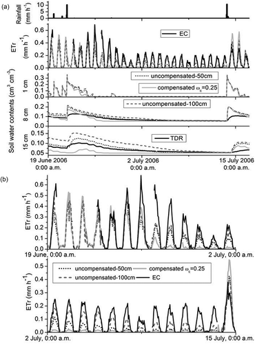
Figure 7. (a) Observed hourly rainfall and real evapotranspiration (ETr) measured by the EC system (EC), soil water contents in the topsoil layer (1 cm) and soil moisture measured by TDR at 8 and 15 cm depth in comparison with those simulated using a rooting depth of 50 cm, uncompensated (uncompensated-50cm) and compensated RWU with ω_c = 0.25 (compensated-50cm ω_c = 0.25) and using a rooting depth of 100 cm (uncompensated-100cm), 21 March 2007, 0:00 a.m. – 10 May 2007, 0:00 a.m., Falkenberg. (b) Hourly ETr, 21 March 2007, 0:00 a.m. – 10 May 2007, 0:00, Falkenberg.

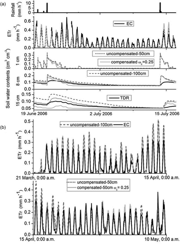
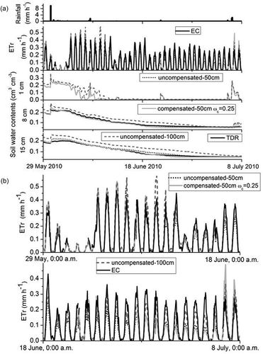
Figure 8. (a) Observed hourly rainfall and real evapotranspiration (ETr) measured by the EC system (EC), soil water contents in the topsoil layer (1 cm) and soil moisture measured by TDR at 8 and 15 cm depth in comparison with those simulated using a rooting depth of 50 cm, uncompensated (uncompensated-50cm) and compensated RWU with ω_c = 0.25 (compensated-50cm ω_c = 0.25) and using a rooting depth of 100 cm (uncompensated-100cm), 29 May 2010, 0:00 a.m. – 8 July 2010, 0:00 a.m., Falkenberg. (b) Hourly ETr, 29 May 2010, 0:00 a.m. – 8 July 2010 0:00 a.m., Falkenberg.

None of our model applications showed an adequate simulation of soil water contents at 90 cm depth throughout the overall investigation period (Fig. 4, Table 6). One explanation of this mismatch between simulated and measured soil water contents at 90 cm depth might be the use of the RWU model with the simplifying assumption of a constant rooting depth of the grass cover. Drought stress can affect vertical distribution of roots of perennial grass cover by increased root growth, which enabled RWU in deeper and wetter soil layers (e.g. Crush et al. 2007, Reid and Crush 2013). Such a water extraction from deeper soil layers by RWU cannot be simulated adequately by assuming a given static root density distribution and constant rooting depth even if RWU compensation is used. Another reason might be measurement errors of the TDR probes installed at 90 cm depth. As previously mentioned, higher deviations between soil water contents determined by field gravimetry and those measured by TDR were observed in soil layers below 45 cm depth. However, these distinct differences in the temporal dynamics of simulated and measured soil water contents at 90 cm depth, mainly in the summer periods from 2004 to 2007 (Fig. 5), could not be explained by measurement errors alone.

The application of RWU compensation resulted in a higher simulated soil water extraction with corresponding soil water contents lower than those calculated by uncompensatory RWU, and those measured by TDR, particularly in the upper root zone above 45 cm depth in the period from 2003 to 2006 (Figs 2 and 4(a)). This caused the lower goodness of fit between measured soil water contents and those calculated using RWU compensation (Table 6).

In other studies with experimental field data obtained from test sites with different soils and vegetation cover, the goodness of fit between simulated and measured soil water contents was described by IA-values of 0.68–0.98, and NS of 0.21–0.93 (e.g. Yang et al. 2009, Deb et al. 2011, 2013, Zhou et al. 2012). Compared to those, the best model performance in our study for soil water contents at 8–45 cm depth in terms of IA was 0.88–0.96 and in terms of NS from 0.48 to 0.84 (Table 6(a)). The results of the model calculations for soil water contents at 60 and 90 cm depths showed lower simulation quality (Figs 2–4, Table 6).

3.2.2 Simulated and measured ETr

Simulated hourly ETr rates in the summer periods ranged mainly above those measured by the EC system (Figs 2 and 3).

The use of RWU compensation resulted in a relative increase of simulated cumulative RWU at an order of magnitude of 3–9%, with the highest increase for the model application using the rooting depth of 100 cm and compensatory RWU with ω_c = 0.25, and with a corresponding decrease in outflow at the lower boundary of the soil profile (Fig. 5).

All model applications using a rooting depth of 100 cm showed better simulation quality for ETr compared to those using a rooting depth of 50 cm (Table 7). RMSD for ETr simulated using a rooting depth of 100 cm, uncompensatory RWU and compensatory RWU with ω_c = 0.75 was 0.04 mm h⁻¹ (Table 7(a,b)), which is similar to the previously discussed uncertainty of the EC measurements at the Falkenberg field site (Mauder et al. 2006). From all these model runs carried out at a rooting depth of 100 cm, the application of uncompensatory RWU resulted in the best fit between simulated and measured ETr described by an IA of 0.94, NS of 0.76, and R² of 0.82 (Table 7(a)).

Table 7. Modelling efficiency index IA, Nash-Sutcliffe index NS, coefficient of determination R² and root mean squared difference RMSD for real evapotranspiration calculated with different model configurations using the 10-year dataset (2003–2012) from the Falkenberg field site.

IA	NS	R^2	RMSD (mm h^−1)
Rooting depth 50/100 cm
(a) Uncompensated root water uptake
0.92/0.94	0.64/0.76	0.73/0.82	0.05/0.04
(b) Compensated root water uptake ωc = 0.75
0.91/0.93	0.62/0.69	0.72/0.79	0.05/0.04
(c) Compensated root water uptake ωc = 0.50
0.91/0.92	0.59/0.66	0.71/0.77	0.05/0.05
(d) Compensated root water uptake ωc = 0.25
0.91/0.92	0.57/0.64	0.70/0.76	0.05/0.05

The lowest model performance for ETr resulted from the use of compensatory RWU with ω_c = 0.25 and 50 cm rooting depth, mainly indicated by a NS of 0.57 (Table 7(d)).

In other studies, such as Izadifar and Elshorbagy (2010) and Vanderborght et al. (2010), the goodness of fit between hourly ETr rates simulated by Hydrus-1D and those measured by EC systems was described by values of R² of 0.50–0.63. Compared to that, the performance of our model applications in terms of R² with values ≥ 0.70 was better (Table 7).

In order to identify reasons for the lower performance of the compensatory RWU model and the deviations between observed and measured ETr rates (Figs.2–4), we analysed two dry periods in 2003 and 2004 in the former study (Wegehenkel and Beyrich 2014). In the present study, we additionally investigated three other dry periods in 2006, 2007 and 2010 (marked by grey circles and black arrows in Figs 2–4). In these dry periods, ETr rates measured by EC were mainly higher than the simulated ones, whereas in wet periods calculated ETr rates were mostly higher than the measured ones.

From the dry year 2006, we selected the period from 19 June to 15 July (Fig. 6). After 21 June 2006, 3:00 p.m., with hourly rainfall of 10 mm, a 26-day period without rainfall led to a decrease of simulated ETr rates to near to zero and of soil water contents at 1 cm depth down to 0.02 cm³ cm⁻³ due to soil water extraction by evaporation and RWU (Fig. 6(a)). This soil water content is equal to a pressure head h_a of 10⁶ cm, which is the threshold for evaporation from the topsoil layer (see Equation (7)). Simulated and measured soil water contents at 8 and 15 cm depth also decreased near to the wilting point, with values of 0.04–0.05 cm³ cm⁻³ (Fig. 6(a), Table 4). After 21 June 2006, ETr rates calculated using the rooting depth of 50 cm and compensatory RWU with ω_c = 0.25 declined rapidly down to values close to or at zero until 2 July 2006, whereas ETr rates simulated by uncompensatory RWU and 50 cm rooting depth decreased to zero a few days later (Fig. 6(b)). In comparison, ETr rates simulated using a rooting depth of 100 cm and uncompensatory RWU also declined to near zero, but distinctly later, until 13 July 2006; these calculated ETr rates were closer to the measured ones than those simulated by the other model applications (Fig. 6(b)). In contrast to the modelling results, measured ETr rates showed a decrease from rates up to 0.75 mm h⁻¹ down to 0.2 mm h⁻¹ until 2 July 2006 and remained more or less constant at this level, despite low measured and simulated soil water contents ≤ 0.04 cm³ cm⁻³ (Fig. 6). In contrast to the modelling results, measured soil water contents at 60 and 90 cm depth indicated RWU in a period from 19 June 2006 to 15 July 2006, which might have contributed to these measured ETr rates. This contribution was simulated insufficiently by all model applications (Figs 4(a) and 6(b)). At the end of this period, the hourly rainfall of 11 mm observed on 13 July 2006, 8:00 p.m., led to a rapid increase of simulated soil water contents and ETr rates (Fig. 6(a)). Compared to that, measured soil water contents were lower and showed only a moderate increase (Fig. 6(a)).

As in the former study (Wegehenkel and Beyrich 2014), hourly ETr rates calculated using compensatory RWU with ω_c = 0.25 switched between rates near or at zero in dry periods lower than those simulated by uncompensatory RWU and measured by EC, and ETr rates in wetter periods distinctly higher than those calculated by uncompensatory RWU and those observed by EC (Fig. 6(b)). One preliminary conclusion in the previous study was that this short-term switching between high and low ETr rates might be due to the value of ω_c = 0.25, which led to stronger soil water depletion of the upper root zone in dry summer periods (Wegehenkel and Beyrich 2014). However, in our recent study, a similar switching between high and low RWU rates was also observed for the application of RWU compensation with ω_c = 0.5 (not shown in Fig. 6(b)). Such a rapid unnatural decrease of RWU under dry conditions of the RWU compensation model used in our study was also observed in the simulation studies of dos Santos et al. (2016) and Peters (2016). This rapid decrease was simulated with values of ω_c < 1 (dos Santos et al. 2016, Peters 2016). However, the results of those two simulation studies were not validated with experimental field data until now. Therefore, the results of the comparisons of simulated with measured hourly ETr rates carried out in our study substantiate the findings of those two simulation studies. In other studies, such as Deb et al. (2011) and Albasha et al. (2015), the application of Hydrus-1D using RWU compensation with values of ω_c ≤ 0.5 also resulted in no meaningful results for ETr and soil water contents. However, the experimental data used in those studies were obtained from test sites with soil types and vegetation cover differing from the conditions of the Falkenberg field site (Deb et al. 2011, Albasha et al. 2015).

In the wet year 2007, a longer period with a low amount of rainfall and corresponding lower soil water contents and ETr rates was observed from March to May. At the beginning of this period, on 21 March 2007, simulated and measured soil water contents at 15 cm depth and above ranged between 0.25 and 0.35 cm³ cm⁻³ (Fig. 7(a)). After hourly rainfall of up to 4.8 mm measured between 22 March and 23 March 2007, a 46-day period with no rainfall was observed until 7 May 2007. During this period, measured and simulated soil water contents decreased to values between 0.02 and 0.04 cm³ cm⁻³ (Fig. 7(a)). Simulated ETr rates ranged above the measured ones until 19 April 2007 (Fig. 7(b)). After this day, measured and simulated ETr rates ranged at the same level without a further decrease of simulated ETr rates, despite low simulated and measured soil water contents (Fig. 7). This was in contrast to the dry year 2006 (Figs 6(b) and 7(b)). At the end of this dry period in 2007, some hourly rainfall of up to 10 mm observed on 7 May 2007 led to a rapid increase of simulated and measured soil water contents (Fig. 7(a)).

From the year with the highest annual precipitation rate, 2010, we chose a period from 29 May to 8 July with a low amount of rainfall and, therefore, lower soil water contents and ETr rates, for a detailed analysis. During this period, after hourly rainfall of 10 mm on 30 May 2010, 12:00 a.m., measured and simulated soil water contents decreased from 0.20–0.30 cm³ cm⁻³ down to 0.02–0.04 cm³ cm⁻³ due to soil water extraction by evaporation and RWU (Fig. 8(a)). After 18 June 2010, measured ETr rates were higher than the simulated ones until some hourly rainfall of up to 2.4 mm observed at the end of this dry period on 6 July 2010 (Fig. 8(b)). During the other months of 2010, rainfall and measured and simulated soil water contents indicated no limitation in soil water availability for evaporation and RWU (Figs 4 and 5(b)).

During wet periods with unlimited soil water availability for RWU and evaporation, hourly ETr rates measured by EC were lower than the simulated ones. In other studies, comparison of hourly and half-hourly ETr rates measured by EC systems with those determined by weighing lysimeters indicated an underestimation of these ETr rates by EC systems due to the well-known energy balance non-closure (e.g. Alfieri et al. 2012, Gebler et al. 2014, Vásquez et al. 2015). Such a non-closure of the energy budget ranging below 25% was also observed at the Falkenberg field site (Foken et al. 2010), which is representative of low-vegetation flux sites. In the study of Foken et al. (2010), this non-closure of the energy budget was analysed in detail, and it was hypothesized that secondary circulations due to small heterogeneities in the surface characteristics (roughness, thermal and moisture properties) might be responsible for the observed non-closure of the energy balance at the Falkenberg test site. We therefore concluded that these lower measured ETr rates were mainly due to the non-closure of the energy budget.

Compared to that, ETr rates measured by EC in dry periods without rainfall and high soil water stress conditions were mainly higher than the simulated ones (Fig. 6). TDR measurements give information about the soil water conditions near the TDR probes at a relatively small plot scale. Compared to that, the footprint of EC measurements can have an extent of more than 100 m, and therefore ETr rates measured by EC are integrated values at field scale. Due to spatial variability in vegetation cover and soil hydraulic properties, areas with higher and lower soil water stress conditions at the same time can be expected at field scale. These areas with lower soil water stress conditions can contribute to ETr measured at field scale by EC. As previously mentioned, a high spatial variability of the depth location of the deepest horizon Bv in the soil profile at field scale was observed for the Falkenberg field site (Beyrich and Mengelkamp 2006). This Bv horizon has lower available water capacity and lower hydraulic conductivity in comparison with the upper two horizons (Tables 2 and 4). Therefore, at areas at the field site with deeper locations of the Bv horizon in the soil profile, a higher amount of water can be stored in the soil in contrast to areas with upper locations of the Bv horizon, resulting in a lower storage capacity for soil water. This is one possible explanation for higher ETr rates measured by EC at the field scale than those simulated by our modelling approaches at the plot scale for dry periods with soil water stress conditions. In a study by Schelde et al. (2011), estimates of ETr based on TDR measurements over dry periods were lower compared with those obtained from EC measurements. In that study, it was hypothesized that ETr rates measured by EC may include minor evaporation of morning dew from the vegetation and rates are therefore higher than those estimated from TDR measurements (Schelde et al. 2011). This could be another explanation for higher ETr rates measured by EC when compared to the simulated ones in dry periods. At the least, simulated ETr rates lower than those determined by EC in dry periods may be also due to an underestimation of RWU from deeper and wetter parts of the root zone at the Falkenberg field site by our modelling approaches. Such a RWU was indicated by the measured soil water contents at 90 cm depth, especially in the dry summer period in 2006 (Fig. 5(a)).

4 Conclusions

The goodness of fit between measured and simulated hourly ETr rates and soil water contents was better than or mainly of the same order of magnitude as that published in other similar studies. This substantiated the applicability of our selected modelling approach for adequate simulation of ETr and soil water contents. In addition, the time series of measured soil water contents and ETr rates from 2003 to 2012 in our study were much longer than those in other cited studies with time periods of experimental data often no longer than 2–3 years. The longer period of 10 years with varying meteorological and soil hydrological conditions enabled a much more thorough model validation as compared to shorter periods of experimental data.

The application of compensatory RWU in our study, especially with the threshold values ω_c ≤ 0.5, led to a decrease in the model performance in terms of NS and IA as compared to the simulation quality achieved by the application of uncompensatory RWU. In addition, the application of RWU compensation with ω_c ≤ 0.5 resulted in a switch between high and low RWU rates with a rapid unnatural decrease of RWU under dry conditions. This shortcoming of the compensatory RWU model was reported in other simulation studies, but had not been validated by experimental field data. This demonstrated the need for a definition of appropriate values of ω_c and for further improvement of compensatory RWU models.

In a previous study, it was also hypothesized that a model-based triggering between the use of compensatory RWU in dry periods and uncompensatory RWU in wetter periods might increase the model performance (Wegehenkel and Beyrich 2014). However, this hypothesis was not confirmed by the results of the long-term analysis in our present study.

All RWU approaches used in our study showed limitations in dry years. Measured soil water contents at 90 cm depth indicated increased root growth and corresponding RWU of the perennial grass cover in deeper and wetter soil layers in the dry years 2003 and 2006. This impact of drought stress in dry years and the corresponding adaption mechanism of perennial grass cover cannot be simulated sufficiently by assuming a given static root density distribution and a fixed maximum rooting depth, even if RWU compensation is used. In general, this indicates the necessity for the measurement of spatial root density distribution in the soil profile and maximum rooting depth at experimental fields with vegetation cover.

In our study, we used time series of hourly ETr rates measured by the EC method without a closure of the energy balance. A comparison of simulated ETr rates with those measured by EC processed with closure of the energy balance should be the subject of a future study.

Disclosure statement

No potential conflict of interest was reported by the authors.

Additional information

Funding

This study was financially supported by the German Federal Ministry of Consumer Protection, Food and Agriculture and the Ministry of Agriculture, Environmental Protection and Regional Planning of the Federal State of Brandenburg (Germany).

References

- Albasha, R., Mailhol, J.-C., and Cheviron, B., 2015. Compensatory uptake functions in empirical macroscopic root water uptake models – Experimental and numerical analysis. Agricultural Water Management, 155, 22–39. doi:10.1016/j.agwat.2015.03.010
- Alfieri, J.G., et al., 2012. On the discrepancy between eddy covariance and lysimetry based flux measurements under strongly advective conditions. Advances in Water Resources, 50, 62–78. doi:10.1016/j.advwatres.2012.07.008
- Allen, R.G., et al., 2011. Evapotranspiration information reporting: I Factors governing measurement accuracy. Agricultural Water Management, 98, 899–920. doi:10.1016/j.agwat.2010.12.015
- Allen, R.G. et al., 1998. Crop evapotranspiration. Guidelines for computing crop water requirements. FAO Irrigation and Drainage Paper No.56. Rome: FAO.
- Beyrich, F. and Adam, W.K., 2007. Site and data report fort he lindenberg reference site in CEOP-phase I. Vol. 230. Offenbach am Main: Berichte des Deutschen Wetterdienstes, 55.
- Beyrich, F., et al., 2006. Area-averaged surface fluxes over the LITFASS-region based on eddy-covariance measurements. Boundary-Layer Meteorology, 121, 33–65. doi:10.1007/s10546-006-9052-x
- Beyrich, F. and Mengelkamp, H., 2006. Evaporation over a heterogeneous land surface: EVA_GRIPS and the LITFASS-2003 experiment - an Overview. Boundary-Layer Meteorology, 121, 5–32. doi:10.1007/s10546-006-9079-z
- Bitteli, M., Salvatorelli, F., and Pisa, P.P, 2008. Correction of TDR-based soil water content measurements in conductive soils. Geoderma, 143, 133–142. doi:10.1016/j.geoderma.2007.10.022
- Braud, I., Varadoa, N., and Olioso, A., 2005. Comparison of root water uptake modules using either the surface energy balance or potential transpiration. Journal of Hydrology, 301, 267–286. doi:10.1016/j.jhydrol.2004.06.033
- Chung, S.-O. and Horton, R., 1987. Soil heat and water flow with a partial surface mulch. Water Resources Research, 23, 2175–2186. doi:10.1029/WR023i012p02175
- Crush, J.R., et al., 2007. Genotypic variation in patterns of root distribution, nitrate interception and response to moisture stress of a perennial ryegrass (Lolium perenne L.) mapping population. Grass Forage Science, 62, 265–273. doi:10.1111/gfs.2007.62.issue-3
- de Willigen, P., et al., 2012. Root water uptake as simulated by three soil water flow models. Vadose Zone Journal, 11. doi:10.2136/vzj2012.0018
- Deb, S.K., Manoj, K.S., and Mexal, J.G., 2011. Numerical modeling of water fluxes in the root zone of a mature pecan orchard. Soil Science Society of America Journal, 75, 1667–1680. doi:10.2136/sssaj2011.0086
- Deb, S.K., et al., 2013. Evaluation of spatial and temporal root water uptake patterns of flood-irrigated pecan tree using the hydrus (2D/3D) model. Journal of Irrigation and Drainage Engineering, 139, 599–611. doi:10.1061/(ASCE)IR.1943-4774.0000611
- Dong, X., et al., 2010. Quantifying root water extraction by rangeland plants through soil water modeling. Plant Soil, 335, 181–198. doi:10.1007/s11104-010-0401-7
- dos Santos, M.A., et al., 2016. Determination of empirical parameters for root water uptake models. Hydrology and Earth System Sciences Discussions, 1–37. doi:10.5194/hess-2016-59
- Evett, S.R., et al., 2012a. Overview of the Bushland Evapotranspiration and Agricultural Remote sensing EXperiment 2008 (BEAREX08): A field experiment evaluating methods for quantifying ET at multiple scales. Advances in Water Resources, 50, 4–19. doi:10.1016/j.advwatres.2012.03.010
- Evett, S.R., et al., 2012b. Soil water sensing for water balance, ET and WUE. Agricultural Water Management, 104, 1–9. doi:10.1016/j.agwat.2011.12.002
- FAO – Unesco, 1988. Soil map of the world. Rom: Food and Agriculture Organization of the United Nations, 119.
- Feddes, R.A., Kowalik, P.J., and Zaradny, H., 1978. Simulation of field water use and crop yield. New York: John Wiley and Sons, 189 pp.
- Foken, T., et al., 2010. Energy balance closure for the LITFASS-2003 experiment. Theoretical and Applied Climatology, 101, 149–160. doi:10.1007/s00704-009-0216-8
- García-Herrera, R., et al., 2010. A review of the European summer heat wave of 2003. Critical Reviews in Environmental Science and Technology, 40, 267–306.
- Gebler, S., et al., 2014. Actual evapotranspiration and precipitation measured by lysimeters: a comparison with eddy covariance and tipping bucket. Hydrology and Earth System Sciences Discussions, 11, 13797–13841. doi:10.5194/hessd-11-13797-2014
- Izadifar, Z. and Elshorbagy, A., 2010. Prediction of hourly actual evapotranspiration using neural networks, genetic programming, and statistical models. Hydrological Processes, 24, 3413–3425. doi:10.1002/hyp.v24:23
- Jarvis, N.J., 2011. Simple physics-based models of compensatory plant water uptake: concepts and eco-hydrological consequences. Hydrology and Earth System Sciences, 15, 3431–3446. doi:10.5194/hess-15-3431-2011
- Katul, G., et al., 2012. Evapotranspiration: A process driving mass transport and energy exchange in the soil-plant-atmosphere-climate system. Reviews of Geophysics, 50. doi:10.1029/2011RG000366
- Kool, D., et al., 2014. A review of approaches for evapotranspiration partitioning. Agricultural and Forest Meteorology, 184, 56–70. doi:10.1016/j.agrformet.2013.09.003
- Kumar, R., Shankar, V., and Jat, M.K., 2015. Evaluation of root water uptake models – a review. ISH Journal of Hydraulic Engineering, 21, 115–124. doi:10.1080/09715010.2014.981955
- Mauder, M., et al., 2006. Processing and quality control of flux data during LITFASS-2003. Boundary-Layer Meteorology, 121, 67–88. doi:10.1007/s10546-006-9094-0
- Mualem, Y., 1976. A new model for predicting the hydraulic conductivity of unsaturated porous media. Water Resources Research, 12, 513–522. doi:10.1029/WR012i003p00513
- Nash, J.E. and Sutcliffe, J.V., 1970. Riverflow forecasting through conceptual models part I — A discussion of principles. Journal of Hydrology, 273, 282–290. doi:10.1016/0022-1694(70)90255-6
- Pereira, L.S., et al., 2015. Crop evapotranspiration estimation with FAO56: past and future. Agricultural Water Management, 147, 4–20. doi:10.1016/j.agwat.2014.07.031
- Peters, A., 2016. Modified conceptual model for compensated root water uptake – a simulation study. Journal of Hydrology, 534, 1–10. doi:10.1016/j.jhydrol.2015.12.047
- Reid, J.B. and Crush, J.R., 2013. Root turnover in pasture species: perennial ryegrass (Lolium perenne L.). Crop and Pasture Science, 64 (2), 165–177. doi:10.1071/CP13079
- Ritchie, J.T., 1972. Model for predicting evaporation from a row crop with incomplete cover. Water Resources Research, 8, 1204–1212. doi:10.1029/WR008i005p01204
- Robinson, D.A., et al., 2008. Soil moisture measurement for ecological and hydrological watershed-scale observatories: a review. Vadose Zone Journal, 7, 358–389. doi:10.2136/vzj2007.0143
- Sándor, R. and Fodor, N., 2012. Simulation of soil temperature dynamics with models using different concepts. The Scientific World Journal, 2012, Article-ID 590287, 1–8. doi:10.1100/2012/590287
- Schelde, K., et al., 2011. Comparing evapotranspiration rates estimated from atmospheric flux and TDR soil moisture measurements. Vadose Zone Journal, 10 (1), 78–83. doi:10.2136/vzj2010.0060
- Shouse, P.J., Ayars, J.E., and Šimůnek, J., 2011. Simulating root water uptake from a shallow saline groundwater resource. Agricultural Water Management, 98, 784–790. doi:10.1016/j.agwat.2010.08.016
- Simunek, J., et al., 2013. The hydrus-1D-software package for simulating the one-dimensional movement of water, heat and multiple solutes in variably saturated media Version 4.17. Riverside, CA: Department of Environmental Sciences, University of California Riverside, 308.
- Soylu, M.E., Kucharik, C.J., and Loheide, S.P., 2014. Influence of groundwater on plant water use and productivity: development of an integrated ecosystem – Variably saturated soil water flow model. Agricultural and Forest Meteorology, 189-190, 198–210. doi:10.1016/j.agrformet.2014.01.019
- Supit, I., Hooijer, A.A., and van Diepen, C.A., 1994. System description of the Wofost 6.0 crop simulation model implemented in CGMS, Vol.1: theory and Algorithms. Luxembourg: Joint Research Centre, Commission of the European Communities, EUR 15956 EN, 146.
- van Genuchten, M., 1980. A closed form equation for predicting the hydraulic conductivity of unsaturated soils. Soil Science Society of America Journal, 44, 892–898. doi:10.2136/sssaj1980.03615995004400050002x
- Vanderborght, J., et al., 2010. Within field variability of bare soil evaporation derived from eddy-covariance measurements. Vadose Zone Journal, 9, 943–954. doi:10.2136/vzj2009.0159
- Vásquez, V., et al., 2015. Integrating lysimeter drainage and eddy covariance flux measurements in a groundwater recharge model. Hydrological Sciences Journal, 60 (9), 1520–1537. doi:10.1080/02626667.2014.904964
- Vogel, T., et al., 2013. Macroscopic modeling of plant water uptake in a forest stand involving root-mediated soil-water redistribution. Vadose Zone Journal, 12. doi:10.2136/vzj2012.0154
- Wegehenkel, M. and Beyrich, F., 2014. Modelling hourly evapotranspiration and soil water content at the grass-covered boundary-layer field site Falkenberg, Germany. Hydrological Sciences Journal, 59, 376–394. doi:10.1080/02626667.2013.835488
- Wegehenkel, M. and Gerke, H.H., 2013. Comparison of real evapotranspiration measured by weighing lysimeters with simulations based on the Penman formula and a crop growth model. Journal of Hydrology and Hydromechanics, 61, 161–172. doi:10.2478/johh-2013-0021
- Willmott, C.J., 1982. Some comments on the evaluation of model performance. Bulletin of the American Meteorological Society, 63, 1309–1313. doi:10.1175/1520-0477(1982)063<1309:SCOTEO>2.0.CO;2
- Yadav, B., Mathur, S., and Siebel, M., 2009. Soil moisture dynamics modeling considering the root compensation mechanism for water uptake by plants. Journal of Hydrologic Engineering, 14 (9), 913–922. doi:10.1061/(ASCE)HE.1943-5584.0000066
- Yang, D., et al., 2009. An easily implemented agro-hydrological procedure with dynamic root simulation for water transfer in the crop–soil system: validation and application. Journal of Hydrology, 370, 177–190. doi:10.1016/j.jhydrol.2009.03.005
- Zhou, J., et al., 2012. Numerical modeling of wheat irrigation using coupled HYDRUS and WOFOST models. Soil Science Society of America Journal, 76, 648–662. doi:10.2136/sssaj2010.0467