Inferring catchment flow path responses using a data-driven model: an exploratory study based on a generalized additive model

ABSTRACT

Identifying physical catchment processes from streamflow data, such as quick- and slow-flow paths, remains challenging. This study is designed to explore whether a flexible nonparametric regression model (generalized additive model, GAM) can be used to infer different flow paths. This assumes that the data relationship in data-driven models is also a reflection of catchment physical processes. The GAM, using time-lagged flow covariates, was fitted to synthetic rainfall–runoff data simulated using simple linear reservoirs. Partial plots of the time-lagged covariates show that the model could differentiate simple and more complex flow paths in simulated synthetic data with short and long memory systems and varying between dry and wet climates. Further analysis of data from real catchments showed that the model could differentiate catchments dominated by slow flow and by quick flow. Therefore, this study indicates that GAM can be used to identify catchment storages and delay processes from streamflow data.

KEYWORDS:

• flow paths
• GAM
• long memory
• short memory
• time lag

Editor R. Woods; Associate editor Q. Zhang

1 Introduction

Recent approaches to improve hydrological model structures have focused on the development of flexible modelling frameworks (Fenicia et al. 2011, 2014, Gupta and Nearing 2014). In these, different model structures aim to represent different flow components arising from different sources (i.e. storages/stores or reservoirs) that may exist in a catchment system. For example, quick- and slow-flow components of the total streamflow can be a combination of flow pathways from several different sources. The quickflow component of streamflow will include direct runoff from rainfall, but may also include older water displaced from soils or groundwater due to recharge on floodplains by hydraulic loadings (Wittenberg and Sivapalan 1999, Hrachowitz et al. 2011, Zabaleta and Antigüedad 2012, Cartwright et al. 2014). The slow-flow (baseflow) component may be composed of regional groundwater, interflow, return flow from bank storage, or even draining of pools on the floodplain (McCallum et al. 2010, Hrachowitz et al. 2011, Cartwright et al. 2014). The contribution of these flow pathways may change over time with varying hydrological conditions. This, in combination with the existence of multiple spatial sources contributing to the flow components, complicates the understanding of catchment processes. Therefore, hydrological models generally restrict the interpretation of the catchment to a limited number of buckets (flow sources) and routing combinations (flow paths).

As a result, identification of flow paths from streamflow records is generally limited to the separation of quickflow and slow-flow paths using graphical separation techniques (Nathan and McMahon 1990), analytical techniques (Cartwright et al. 2014), rainfall–runoff models (Dye and Croke 2003), data-based mechanistic models (Young 2003) and baseflow filters (Nathan and McMahon 1990, Eckhardt 2005). Essentially, most of these techniques make use of underlying algorithms or fitting procedures to identify the quick- and slow-flow components from the streamflow, with the exception of those methods where interflow is also detected (e.g. Willems 2009).

Other methods, such as those using geochemistry data (e.g. electrical conductivity, major ions, stable and radiogenic isotopes, gases, nutrients and contaminants), can identify varying concentrations of different flow components on the rising limb of the hydrograph relative to the falling limb of the hydrograph (Cartwright et al. 2014). This information can be further used to identify different sources of the flow paths contributing to the streamflow and varying over time (e.g. Evans and Davies 1998, Tardy et al. 2004, 2005, Aubert et al. 2013, Cartwright et al. 2014). However, due to costs and difficulty of sampling, geochemistry data are generally limited to a short temporal period, discontinuous and often collected during low-flow periods (Lessels and Bishop 2015). In contrast to geochemical data, streamflow data are usually available for longer periods and are continuous. Furthermore, streamflow represents the aggregated hydrological response of a catchment (Basu et al. 2011).

Data-driven modelling has been used for more than two decades in hydrological modelling (Elshorbagy et al. 2010). Data-driven models are empirical, black-box models that relate hydrological variables through a set of empirical functions, mathematical expressions or time series equations (Remesan and Mathew 2015). Amongst the hydrological data-driven modelling techniques, time series models, such as autoregressive integrated moving average models (ARIMA), generalized least squares (ARMAX) and artificial neural network (ANN) techniques, are most popular and mainly used for forecasting or generation of stochastic time series data (Lohani et al. 2012). However, being purely empirical approaches, these techniques may provide little insight into the hydrological behaviour of a system (Lees 2000). The IHACRES model (Jakeman et al. 1990, Jakeman and Hornberger 1993) can be seen as a hybrid, and lies at the boundary between data-driven modelling and conceptual hydrological modelling. In this model, streamflow separation into quickflow and slow-flow components is via a linear module. After a nonlinear conceptual module transforms rainfall into rainfall excess, a linear data-driven transfer function transforms rainfall excess into streamflow.

Only a few studies have attempted to justify the physical basis of empirical model structures from catchment processes, for example, Salas and Smith (1981), based on time series models; Young and Beven, based on a data-based mechanistic model (DBM); and, more recently, Jain et al. (2004), based on ANNs. However, the nature of the stochastic model formulation and physical interpretation of the model components varies greatly between these approaches. For example, ARIMA, ARMAX and ANN models are formulated based on the memory of a catchment by including time-lagged streamflow in the model structure (Hipel and McLeod 1994, Shook et al. 2015). The DBM approach leads to more customized determination of catchment storage and flow separations than the more generic ARIMA and ANN models. Both the DBM and ARIMA assume a generic model transfer function, for which the parameters are adapted based on the observed data. In contrast, ANN does not assume any generic transfer function but uses a sigmoid transfer function as the activation function for both the hidden and the output layers (Jain et al. 2004).

Building on this earlier research, it may be useful to use a data-driven approach based on the sequence of time-lagged streamflow events to represent the storage and delay response behaviour of the catchment (Laurenson 1964). Therefore, the aim of this research is to use a data-driven approach to disaggregate the streamflow data into the different contributing flow paths. Rather than functioning as a purely predictive approach, this has the potential to improve our understanding of catchment processes and identify also how catchment processes may be changing as a result of changes in climate and land use.

2 Methods

2.1 Generalized additive models (GAMs)

In this paper, we use generalized additive models (GAMs) (Hastie and Tibshirani 1990), which are semi-parametric models that can combine linear and smooth relationships between predictor and response variables. This is useful to capture nonlinear patterns and non-monotonic relationships in the data without having to specify detailed parametric relationships in the model (Richards et al. 2010). Furthermore, a GAM is more or less similar to a DBM in terms of model parameter estimation (using a standard back-fitting algorithm) and order selection via the Akaike information criterion (AIC) or Bayesian information criterion (BIC). Furthermore, cross-validation can be used to detect or reduce overfitting problems. Moreover, the backshift operator is based on polynomials in GAM and can be interpreted as nonlinear smoothers similar to the DBM functions (Young 2003).

In the general form of the GAM model the response variable (g) on the link scale is expressed as the sum of individual univariate nonparametric smoothing functions. Each of the nonparametric functions can be considered as the effect of the corresponding input, while taking other inputs as constant:

(1)

where l is the link function, a₀ is the intercept, and f_{1, …, j} are the nonparametric smoothing functions for variable x_{1, …, i} (Wood 2006). The nonparametric function is estimated in a flexible manner using smoothing splines. For example, the function f(x_i) is of the form , where b_m(x_i) for m = 1, …, M are a set of basis functions, and are the parameters to be estimated (Wood 2006). A further advantage is that the model is generalized and therefore the response variable may be drawn from a number of families of distributions, for example, Poisson, gamma, Gaussian and inverse Gaussian.

The systematic component of a GAM may consist of several different covariates (Equation (2)). These can be included as linear terms, smooth functions, or as a smooth surface capturing an interaction between two continuous covariates (Underwood 2009):

(2)

where x₁ … x₄ are four covariates. The covariate x₁ is a linear term, whilst x₂ is fitted with a nonparametric smoothing function (f), and x₃ and x₄ are fitted with a nonparametric smooth surface (h).

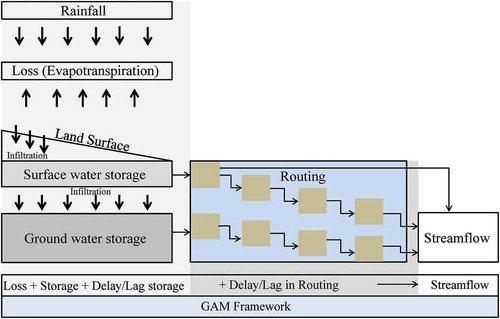
In this study, all catchment processes are conceptualized as a combination of storage, routing and loss processes after the Thomas-Fiering model (Thomas and Fiering 1962, Salas and Smith 1981) and this can be portrayed in a GAM model (Fig. 1 and Equation (3)) using time-lagged streamflow and rainfall as predictor variables in the model. Therefore, the predictor variables in the GAM model represent: (a) input; (b) loss, storage and delays/lag through groundwater and surface water storage; and (c) delays and lags through the routing process of the catchment:

(3)

Figure 1. Generalized GAM framework and corresponding catchment conceptualization.

where t is time, and i and j represent the smoothed ith and jth lagged rainfall and streamflow covariates. The streamflow data were log-transformed and the few zero values in the data were ignored in the model fitting procedure. The models were fitted using the package “mgcv” in R and the default thin-plate regression spline was used for the smoothing functions (Wood 2006, R Core Team 2014).

2.2 Virtual catchment model experiment

To demonstrate how different catchment stores generate memory and how this will materialize in the partial GAM, a virtual catchment model experiment was developed first. Streamflow (Q_t) was generated using two simple daily catchment models (Fig. 2). The rainfall input (P) is interpreted as the effective rainfall input, which means the model only represents the routing component of a typical rainfall–runoff model. The first model (Equation (4), Model1) consists of simple quick- and slow-flow paths, each modelled with a linear store functioning as a discrete unit hydrograph model working on the rainfall input. The partitioning of the flow between the different stores is governed by a parameter w. The second model (Equation (5), Model2) consists of three stores, (again modelled as a discrete unit hydrograph model), where the second and third stores are in series in the slow-flow path. This last part represents a two-store Nash cascade (Nash 1957), and again the partitioning of the flow between the quick- and slow-flow paths was governed by w. The recession constants (k_f and k_s) of the linear stores were fixed at 0.8 for the fast-flow path and 0.05 for the slow-flow path, relating to residence times of 1.25 and 20 days, respectively, and the time step (t) is daily.

(4)

(5)

Figure 2. Schematic diagram of the tested virtual catchment models.

In Equations (4) and (5), t is the time for the runoff series, and τ is the time in the precipitation time series. Rainfall (5000 days) was generated with a simple exponential rainfall generator (Vervoort and van der Zee 2008), with two parameters: the mean rainfall depth and the mean number of storms per day. A long rainfall series was used to ensure sufficient degrees of freedom in the fitting of the GAM models. Rainfall for a number of climates was generated. The mean rainfall depth was set to 10 mm and the mean number of storms was set to 0.5 storms per day for the climate with the most frequent rainfall. Climates with less frequent rainfall were simulated by setting the mean number of storms to 0.30 and 0.15, and the mean rainfall depth was adjusted to ensure that the total volume of rainfall was the same for all of the simulated climates. To ensure independence, each of the generated rainfall series was tested by looking at an autocorrelation function (ACF) and checking whether any of the lagged correlations were significant.

Flows were generated for the two models and for two values of w. Values for w were arbitrarily chosen, but sufficiently far apart such that w = 0.2 represents a slow-flow dominated system and w = 0.8, a quickflow dominated system.

The generated streamflow data were fitted with a GAM (Equation (3)). Lagged streamflow of up to 30 days and lagged rainfall of up to 10 days were included in the models. Nonsignificant lagged predictor variables were dropped from the model using backward elimination (p < 0.001). The chosen p value (0.001) is rather conservative, which may lead to a Type II error. However, it was decided that this would select covariates representing the main processes in the model. A further simulation was conducted to test whether the models chose the significant lags consistently. To test selection consistency, 1000 random rainfall series were generated for the frequent (wet) and less frequent (dry) rainfall scenarios, and both Model1 and Model2 were run for both the quickflow and slow-flow scenarios. The selection frequency of significant lags was recorded for the 1000 simulations. Furthermore, the model performance was also evaluated in terms of flow duration curves (FDCs) of synthetic (observed) flow and simulated flow with the KGE (Kling-Gupta efficiency) statistic (Kling et al. 2012). The FDC was chosen as it enables model evaluation for different flow signals (high-, mid- and slow-flow signals). Furthermore, the KGE provides diagnostic insight into the model performance by decomposing into correlation (r), bias ratio (β) and variability ratio (γ). Therefore, the temporal dynamics and preservation of the flow distribution can all be evaluated. The optimum value of KGE is unity and takes the following form:

(6)

where μ is the mean runoff, CV is the coefficient of variation, and the indices s and o represent simulated and observed flows, respectively.

2.3 Demonstration with real catchments

To compare the results of the virtual experiment to real catchments, a GAM was also fitted to real streamflow data. Seven hydrological reference stations (Turner et al. 2012) were selected from various locations around Australia. The locations were mainly selected to represent a range of climates, a range of flow characteristics and a range of catchment properties. The selected stations are summarized in Table 1 and locations of the stations are shown in Figure 3. Twelve years of daily data were used to capture sufficient temporal flow variation. Similar to the virtual experiment, the GAM model was fitted using several time-lagged streamflow and rainfall series as covariates, and nonsignificant lagged covariates were dropped from the model.

Table 1. Flow summaries of selected Australian stations based on daily data for the period 2000–2011. Station information can be accessed at http://www.bom.gov.au/water/hrs/. Min: minimum; and Max: maximum.

Station	Catchment size (km^2)	Mean rainfall (mm)	Min flow (m^3/s)	Max flow (m^3/s)	Mean flow (m^3/s)	Latitude	Longitude	State
A5030502	29.00	772.80	0.00	6.10	0.10	−35.1013	138.6730	South Australia
607155	115.70	1231.80	0.00	37.17	1.10	−34.5787	115.9723	Western Australia
G9030250	134.42	896.00	0.91	39.75	174.30	−14.6980	134.4180	Northern Territory
304499	210.20	1163.60	0.37	64.17	5.43	−42.7083	146.7083	Tasmania
308145	775.30	2550.40	2.71	681.20	45.79	−42.2433	145.7683	Tasmania
G8140001	8356.80	971.20	0.20	4563.00	107.60	−14.4650	132.2570	Northern Territory
A0020101	119033.60	164.90	0.00	1975.00	57.50	−25.9085	139.3670	South Australia

Figure 3. Map showing the location of the hydrological reference stations used in the study.

3 Results and discussion

3.1 Virtual catchment experiment results

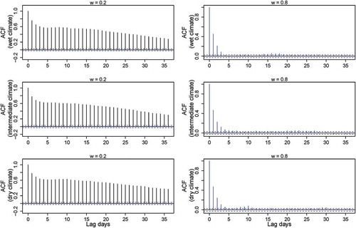
The quickflow path from the virtual model clearly showed short memory, while the slow-flow path showed long memory for all types of rainfall (frequent and less frequent) (see Appendix). This confirms that the models generated memory from the uncorrelated rainfall data, and that the memory is varied by flow path and process.

The fitted GAM models on the synthetic data showed satisfactory model performance (KGE = 0.93–0.97) (see Appendix, Figs. A1 and A2), which indicates that the results from the models can be confidently interpreted to understand store behaviours and flow paths. However, at higher percentiles for very low flows, or zero-flow events that are purely random in nature, the GAM struggles. Such random process may not be the same for other flow events. However, it appears that in a slow-flow system the predictions of Model2, with frequent rainfall climate (Appendix, Fig. A2), at higher percentiles are very satisfactory. The longest significant lag found for rainfall was just 1 day. This is logical as the memory in the rainfall is small and the generated memory in the stores is most likely captured by the lagged flow variables.

3.1.1 Results from the slow- and quickflow dominated flow systems

The GAMs fitted to the slow-flow dominated models (w = 0.2) generally indicated several longer time-lagged streamflow variables to be significant (Figs. 4 and 5, bottom panels). This suggests that the simulated flow series had long memory, introduced by the linear reservoir(s). The only exception was in the scenario with less frequent rainfall. This “dry” scenario showed longer dry spell lengths and thus rainfall that was more irregularly distributed in time. Therefore, generated flows from Model1 and Model2 resulted in an irregular selection of significant lag periods in the GAM. This suggests that the frequency of the input pulses into a single linear reservoir also has an effect on the autocorrelation of the streamflow. The ACFs of generated flow also show different levels of autocorrelation in the simulated flow, but mainly between the models and between the different levels of parameter w (see Appendix, Figs. A3 and A4).

Figure 4. Significant time-lagged flows for Model1. Top row: Mod1.Q, a fast-flow dominated system (w = 0.8), and bottom row: Mod1.S, a slow-flow dominated system (w = 0.2); from left to right: frequent (wet), intermediate and less frequent (dry) rainfall climate.

Figure 5. Significant time-lagged flows for Model2. Top row: Mod2.Q, a fast-flow dominated system (w = 0.8), and the bottom row: Mod2.S, a slow-flow dominated system (w = 0.2); from left to right: frequent (wet), intermediate and less frequent (dry) rainfall climate.

For the quickflow dominated models, i.e. with w = 0.8 (Figs. 4 and 5, upper panels), the fitted GAM models only identified flow at 1-, 2- and 3-day lags, and rainfall at zero lags as being significant for different rainfall frequency scenarios. However, in both models, flows at 8-, 10- and 12-day lags were also significant. This unexpected selection might be attributed to the synthetic data distribution and perhaps may be ignored. This is tested in the next section.

In summary, the number of reservoirs and the distribution of flow through the slow- or quickflow paths had a marked effect on streamflow memory. The frequency and intensity of rainfall did not significantly affect streamflow memory. This is an important result as it demonstrates the capacity of these simple conceptual catchments to smooth the rainfall signature and may indicate why natural streamflow remains unchanged under a scenario where rainfall intensity is increasing and the frequency is decreasing.

3.1.2 Validating the lag selection from the GAM model

Figure 6 shows the distribution of selected significant time-lagged flows of the quickflow system (w = 0.8) for 1000 runs of Model1 and Model2 in the “wet” and “dry” scenarios. Selection of significant time-lagged flows is quite stable and quite similar for both models. This suggests the selection of significant time-lagged flows is similar, irrespective of the delays introduced by the number of storages from different models. The “wet” scenario models show a marginal increase in the number of lags appearing, with lag times greater than 4 days.

Figure 6. Significant time-lagged flows in a fast-flow system (w = 0.8) from the randomly simulated rainfall (1000 samples) for Model1 (top) and Model2 (bottom) for wet (left) and dry (right) climates.

Figure 7 shows the distribution of significant time-lagged flows selected for the slow-flow system (w = 0.2) of 1000 runs of Model1 and Model2 in the “wet” and “dry” scenarios. In contrast to the quickflow system, longer time-lagged flows are being regularly selected for the slow-flow system and more so under the “wet” scenario. The three-cascade model (Model2) for this scenario demonstrates the effect of delay in the slow-flow system, and indicates long memory and a contribution from the additional store. In comparison, fewer long-time lags were selected for the two-cascade model (Model1), but there were still more significant longer lags than in the quickflow systems (w = 0.8, Fig. 6). In the “dry” scenarios, fewer time lags are selected than in the “wet” scenario, indicating shorter memory and a response dominated by surface runoff.

Figure 7. Significant time-lagged flows in a slow-flow system (w = 0.2) from the randomly simulated rainfall (1000 samples) for Model1 (top) and Model2 (bottom) for wet (left) and dry (right) rainfall climates.

The simulation results using random rainfall therefore suggest that the distribution of significant time-lagged streamflow selected in the GAM model is related to the response behaviour (flow paths) of the catchment. Therefore, a real catchment with a fast-flow dominated system is likely to have less memory in the flow, leading to shorter flow path selection (shorter selected lag periods) in a GAM model. In contrast, for a slow-flow dominated system, there is likely to be more memory, leading to longer flow path selection (longer lag periods in the GAM).

3.1.3 Flow response behaviour

Once significant time-lagged flows have been selected in the GAM, their impulse response functions can be linked to catchment hydrology. Essentially, these impulse response functions of the time-lagged flows are characteristic of the shape of the hydrograph of a rainfall–runoff event (Fig. 8). These plots map the contribution of the individual time-lagged flow variables to the total flow response, thus representing a component of the overall flow behaviour of the system. For the fast-flow dominated system (w = 0.8) in Model1, only lag1 flow contributes significantly to the total streamflow (Fig. 8). Contributions from longer time-lagged flows are minor, as indicated by the almost flat horizontal response curves centred on the mean flow.

Figure 8. Response behaviour of Model1 with a fast-flow dominated system for wet, intermediate and dry climates (from top to bottom, respectively). Grey shading represents the standard error boundary. Suffix of “lag” indicates number of days of time lag.

Interestingly, there seem to be three main general shapes in the response curves in the virtual modelling: (a) a log-shaped curve, such as in the lag1 response for the frequent rainfall scenario (Fig. 9, top row); (b) an exponential rising curve, such as in the lag1 response for the infrequent rainfall scenario (Fig. 9, bottom row); and (c) a decreasing curve, such as in the lag2 response curve for the infrequent rainfall scenario (Fig. 9, bottom row). Specifically, the shape of the response (resembling a log curve) for the lag1 flow in the frequent rainfall scenario appears opposite to the response for the equivalent time-lagged flow in the infrequent rainfall.

Figure 9. Variation in catchment responses to the input events based on the response curves. Grey bars are rainfall input.

The log-shaped curve (a) would be logical for the drainage of a linear reservoir, which declines exponentially. In general, this sort of response curve results in a typical hydrograph shape in the flow curve with a significant recession (Fig. 10). Larger (time-lagged) flows would be related to larger events, while for smaller flow events the response to the time-lagged flows is smaller. Most of the lag1 curves are in fact log shaped, and therefore represent the main typical linear reservoir response from the virtual model catchments.

Figure 10. Response behaviour of Model1 with a slow-flow dominated system for wet, intermediate and dry climates (from top to bottom). Grey shading represents the standard error boundary.

In contrast, the exponential increasing curve (b) shows a peakier response to the flow. For short time-lagged flow (lag1), this is similar to a typical arid/semi-arid flashy response system. For the larger lags (for example, lag3 in the frequent rainfall scenario and lag10 in the less frequent rainfall scenario), this is accompanied by a shift in time of the response (Fig. 10). This all leads to short recession times for these responses.

Finally, a decreasing curve (c), either linear or nonlinear, indicates a typical baseflow signature with a decreased flow response related to the peak events and a slowly increasing flow response for smaller lag flow events (Fig. 10).

Comparing the flow responses for Model1 of the slow-flow dominated system (Fig. 10, with w = 0.2), with those of the quickflow dominated system (Fig. 8), we can again observe that for all scenarios the lag1 response is a log response, or a traditional hydrograph. However, moving from more frequent, less intense rainfall to less frequent, more intense rainfall, the curve flattens, thus leading to a more even response for all flow events. In addition, for the greater lags in the less frequent rainfall scenarios, peakier responses (concave exponential responses) are observed, with therefore short recessions. In contrast, for the frequent rainfall system, most of the higher lag responses are generally flat or slightly convex, suggesting a smoother hydrograph response with a longer recession.

The Model2 responses for both the fast- and slow-flow dominated systems were similar to the Model1 responses. The main difference, however, was in the number of days of time lag that were identified as significant, as already indicated in Figures 4 and 5.

The interesting finding of the virtual experiments is that longer lags or long flow paths (i.e. parts of the hydrograph representing long memory) still indicate quite short recession responses, rather than being smoothed signals.

3.2 Results from the real catchments

For the real catchments, different time-lagged flows were significant for different catchments (Table 2). Based on the results from the virtual experiments, this suggests both long and short memory processes, but also indicates the different types of recessions (in particular, short and long recessions, Fig. 9).

Table 2. Flow characteristics of real catchments.

Catchment ID	Catchment size (km^2)	Mean flow (m^3/s)	Significant time lags (days)	Response curve types
A5030502	29.00	0.10	1, 2, 6, 10, 25, 60	a, c and b
607155	115.70	1.10	1, 2, 3, 4, 17, 18, 24, 38, 39, 40	a, b, c and combination of a, b and c
G9030250	134.42	174.30	1, 2, 28, 29, 44, 45, 46, 59, 60	Type a, b, c and combination of a, b and c
G8140001	210.20	5.43	1, 2, 10	a, c and combination of a and c
304499	775.30	45.79	1, 2, 3, 23, 30	a, c and combination of c and a
308145	8356.80	107.60	1, 2, 3	a, c and combination of a and c
A0020101	119033.60	57.50	1, 2	a and c

The 1- and 2-day time-lagged streamflow covariate was significant in the GAM models for all catchments. All 1-day time-lagged (lag1) flows had monotonically increasing response curves that formed a log-shaped curve (Type a, Fig. 9). The 2-day time-lagged flows (lag2) generally showed a sharp exponential decay response (related to Type c, Fig. 9). As indicated, this relates to a typical baseflow response with low contributions during high-flow periods and high contributions during low-flow periods. For those catchments where the 3-day lagged flow was significant, the shape was again a log curve (Type a, Fig. 9).

Longer time-lagged flow response curves showed complex behaviours, and the contribution to streamflow was generally less than shorter lags and often almost linear. A key observation is that consecutive lags tend to show almost opposite behaviours. In particular, Type b is often followed directly by 1/(Type a), or vice versa, or Type a is often followed by Type c. Currently, it is not exactly clear how these types of response curves can be interpreted in terms of catchment physical processes. This is an avenue for further research, which will be outlined further in the discussion.

Table 2 summarizes the response classifications for real catchments based on Figure 9. A key observation is that the shapes of the smoothed lag flow covariates of the observed data are quite different from those of the modelled flow. The observed and modelled flow both show a Type a relationship at lag1, but the increase is much more gradual in the modelled data. In contrast, the lag2 flow shows a Type c relationship in the observed data, and a very flat Type a relationship in the modelled data. This clearly suggests that our process-based virtual models are overly simplistic and are not able to capture the pattern of flow that appears to be fairly consistent over the diverse range of catchments selected in this study.

The other aspect to consider is the number of lags selected in the backward elimination process (Table 2). It is tempting to classify the catchments based on the number of lags selected, but this is beyond the scope of this study, as it would require a much larger sample size. However, qualitatively it appears that only short lags were selected for the two large catchments compared to the smaller catchments. This could be because the response time is actually much slower in the larger catchments and therefore we would have to increase the maximum lag time beyond 60 days to detect this. A much more thorough study comparing detailed catchment characteristics and lag flow characteristics would need to be undertaken to confirm this. Such a study would also be useful for determining other catchment characteristics that may correlate with the lagged flow characteristics and the shapes of the response curves.

Interestingly, the larger catchments behaved more like Model1 (quickflow dominated) and all rainfall scenarios, while the smaller catchments behaved more like Model2 (slow-flow dominated with additional storage) and the frequent rainfall scenario. Due to the small sample size of observed catchments, it is not clear whether this is indeed a trend. However, this is something that could be tested with a large number of catchments.

4 General discussion

Findings from this exploratory modelling study indicate that, in contrast to other data-driven models (discussed in Section 1), nonlinear regression modelling with GAM can be a useful approach to understand the flow paths (in particular, slow- and quickflow paths) of a catchment across different climates. This is useful to assist with the conceptualization and parameterization of more complex or physically-based models. However, the complex behaviour of the catchment process responses is still not fully obvious from the approach presented here and this requires further research. In particular, the study did not specifically separate variations in the quick- and slow-flow paths between the surface or subsurface, rather it only distinguished between slow and fast flows. This separation might be important as it would be related to short memory and long memory. The results from the real catchments already showed that flow-path behaviour, as shown in Figure 9, becomes more complex, and possibly understanding how surface and subsurface interact might explain some of the variation. Further, this study has not explicitly established the number of stores specific to the catchment. However, as discussed in Section 1, different flow paths are in fact the result of different transient stores in a catchment. From the current experiment, the selected number of time-lagged flows (identified as flow paths) can be thought of as the number of transient stores, which can be set up either in parallel or in series to form a model structure for investigating flow generation.

In addition, this study is limited by exactly how many time-lagged flows are selected, which may vary for longer lag periods (for example 15-day or 16-day time-lagged flows may have equal impact and still can be selected as significant by the model). This is because both might have a p value < 0.001. In such case, the PACF might help to single out dominant time-lagged flow days. Nevertheless, a small experiment shows (results not presented) that only relying on PACF for lag day selection would be misleading, in particular for frequent rainfall climates and for slow-flow dominant systems. Additional variation in the modelling result could arise from the selection of knot size for the GAM model and the specific error distribution function. However, variation from this appears minor and was ignored given the focus of the study.

5 Conclusions

This study shows the statistical GAM was able to infer the structure of flow paths from simple rainfall–runoff models. This means the GAM can in principle provide information about the catchment functioning and memory systems, and demonstrate how the storage response from the catchment shifts between long-memory and short-memory flow paths. There were clear differences between the response curves in the GAMs fitted to the observed data and modelled data, indicating that the simple models are not complex enough to reproduce the complexities of the contributions of different stores to streamflow. However, the lagged flows selected by the GAMs were similar in both the observed and modelled data. This may suggest that the simplistic models may reasonably represent the stores, but the function governing the way the store is operating is not correct. This means that this research direction can be used to improve our understanding of catchment hydrology by disaggregating observed streamflow and rainfall data. A clear application would be to compare simulated and observed streamflow signatures in order to determine whether a chosen simulation model is capturing the complexity of the natural catchment.

Acknowledgements

D. Kundu received the F.H. Loxton postgraduate award, The University of Sydney, Australia. The authors are grateful for constructive comments from anonymous reviewers that helped to improve the quality of the paper.

Disclosure statement

No potential conflict of interest was reported by the authors.

Appendix

Figure A1. Flow duration curves of observed vs predicted (1-day ahead) flows. Mod1: Model1; Mod2: Model2; Q: the fast-flow system (w = 0.8); Wet: the most frequent rainfall climate; med: the intermediate climate; and dry: the less frequent rainfall climate. KGE: Kling-Gupta efficiency.

Figure A2. Flow duration curves of observed vs predicted (1-day ahead) flows. See Figure A1 for explanation of abbreviations.

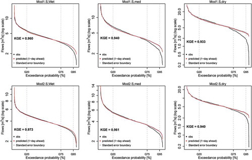
Figure A3. ACFs of streamflow generated for Model1 with slow-flow (w = 0.2, left column) and fast-flow (w = 0.8, right column) dominated systems.

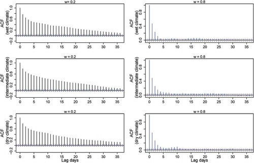
Figure A4. ACFs of streamflow generated for Model2 with slow-flow (w = 0.2, left column) and fast-flow (w = 0.8, right column) dominated systems.

References

- Aubert, A.H., Gascuel-Odoux, C., and Merot, P., 2013. Annual hysteresis of water quality: A method to analyse the effect of intra- and inter-annual climatic conditions. Journal of Hydrology, 478, 29–39. doi:10.1016/j.jhydrol.2012.11.027
- Basu, N.B., Thompson, S.E., and Rao, P.S.C., 2011. Hydrologic and biogeochemical functioning of intensively managed catchments: A synthesis of top-down analyses. Water Resources Research, 47 (10), W00J15. doi:10.1029/2011WR010800
- Cartwright, I., Gilfedder, B., and Hofmann, H., 2014. Contrasts between estimates of baseflow help discern multiple sources of water contributing to rivers. Hydrology and Earth System Sciences, 18 (1), 15–30. doi:10.5194/hess-18-15-2014
- Dye, P.J. and Croke, B.F., 2003. Evaluation of streamflow predictions by the IHACRES rainfall–runoff model in two South African catchments. Environmental Modelling & Software, 18 (8), 705–712. doi:10.1016/S1364-8152(03)00072-0
- Eckhardt, K., 2005. How to construct recursive digital filters for baseflow separation. Hydrological Processes, 19 (2), 507–515. doi:10.1002/(ISSN)1099-1085
- Elshorbagy, A., et al., 2010. Experimental investigation of the predictive capabilities of data driven modeling techniques in hydrology - Part 1: concepts and methodology. Hydrology and Earth System Sciences, 14 (10), 1931–1941. doi:10.5194/hess-14-1931-2010
- Evans, C. and Davies, T.D., 1998. Causes of concentration/discharge hysteresis and its potential as a tool for analysis of episode hydrochemistry. Water Resources Research, 34 (1), 129–137. doi:10.1029/97WR01881
- Fenicia, F., Kavetski, D., and Savenije, H.H.G., 2011. Elements of a flexible approach for conceptual hydrological modeling: 1. Motivation and theoretical development. Water Resources Research, 47 (11), n/a-n/a. doi:10.1029/2010WR010174
- Fenicia, F., et al., 2014. Catchment properties, function, and conceptual model representation: is there a correspondence? Hydrological Processes, 28 (4), 2451–2467. doi:10.1002/hyp.9726
- Gupta, H.V. and Nearing, G.S., 2014. Debates-the future of hydrological sciences: A (common) path forward? Using models and data to learn: A systems theoretic perspective on the future of hydrological science. Water Resources Research, 50 (6), 5351–5359. doi:10.1002/2013WR015096
- Hastie, T.J. and Tibshirani, R.J., 1990. Generalized additive models. Boca Raton, FL: Taylor & Francis.
- Hipel, K.W. and McLeod, A.I., 1994. Time series modelling of water resources and environmental systems. Amsterdam: Elsevier.
- Hrachowitz, M., et al., 2011. On the value of combined event runoff and tracer analysis to improve understanding of catchment functioning in a data-scarce semi-arid area. Hydrology and Earth System Sciences, 15 (6), 2007–2024. doi:10.5194/hess-15-2007-2011
- Jain, A., Sudheer, K.P., and Srinivasulu, S., 2004. Identification of physical processes inherent in artificial neural network rainfall runoff models. Hydrological Processes, 18 (3), 571–581. doi:10.1002/(ISSN)1099-1085
- Jakeman, A.J. and Hornberger, G.M., 1993. How much complexity is warranted in a rainfall–runoff model? Water Resources Research, 29 (8), 2637–2649. doi:10.1029/93WR00877
- Jakeman, A.J., Littlewood, I.G., and Whitehead, P.G., 1990. Computation of the instantaneous unit hydrograph and identifiable component flows with application to two small upland catchments. Journal of Hydrology, 117 (1–4), 275–300. doi:10.1016/0022-1694(90)90097-H
- Kling, H., Fuchs, M., and Paulin, M., 2012. Runoff conditions in the upper Danube basin under an ensemble of climate change scenarios. Journal of Hydrology, 424-425, 264–277. doi:10.1016/j.jhydrol.2012.01.011
- Laurenson, E.M., 1964. A catchment storage model for runoff routing. Journal of Hydrology, 2 (2), 141–163. doi:10.1016/0022-1694(64)90025-3
- Lees, M.J., 2000. Data-based mechanistic modelling and forecasting of hydrological systems. Journal of Hydroinformatics, 2 (1), 15–34.
- Lessels, J.S. and Bishop, T.F.A., 2015. A simulation based approach to quantify the difference between event-based and routine water quality monitoring schemes. Journal of Hydrology: Regional Studies, 4, 439–451.
- Lohani, A.K., Kumar, R., and Singh, R.D., 2012. Hydrological time series modeling: A comparison between adaptive neuro-fuzzy, neural network and autoregressive techniques. Journal of Hydrology, 442-443, 23–35. doi:10.1016/j.jhydrol.2012.03.031
- McCallum, J.L., et al., 2010. Solute dynamics during bank storage flows and implications for chemical base flow separation. Water Resources Research, 46, 7. doi:10.1029/2009WR008539
- Nash, J., 1957. The form of the instantaneous unit hydrograph. Comptes Rendus Et Rapports Assemblee Generale De Toronto, 3, 114–121.
- Nathan, R. and McMahon, T., 1990. Evaluation of automated techniques for base flow and recession analyses. Water Resources Research, 26 (7), 1465–1473. doi:10.1029/WR026i007p01465
- R Core Team, 2014. R: A Language and Environment for Statistical Computing, R Foundation for Statistical Computing. Vienna, Austria (www.R-project.org).
- Remesan, R. and Mathew, J., 2015. Hydroinformatics and data-based modelling issues in hydrology. Hydrological data driven modelling: a case study approach. Cham: Springer International Publishing. 19–39.
- Richards, R.G., et al., 2010. Using generalized additive models to assess, explore and unify environmental monitoring datasets. In: D.A. Swayne, ed. International congress on environmental modelling and software. Ottawa, ON: IEMSs.
- Salas, J.D. and Smith, R.A., 1981. Physical basis of stochastic-models of annual flows. Water Resources Research, 17 (2), 428–430. doi:10.1029/WR017i002p00428
- Shook, K., Pomeroy, J., and van der Kamp, G., 2015. The transformation of frequency distributions of winter precipitation to spring streamflow probabilities in cold regions; case studies from the Canadian Prairies. Journal of Hydrology, 521, 395–409. doi:10.1016/j.jhydrol.2014.12.014
- Tardy, Y., Bustillo, V., and Boeglin, J.-L., 2004. Geochemistry applied to the watershed survey. Applied Geochemistry, 19 (4), 469–518. doi:10.1016/j.apgeochem.2003.07.003
- Tardy, Y., et al., 2005. The Amazon. Bio-geochemistry applied to river basin management. Applied Geochemistry, 20 (9), 1746–1829. doi:10.1016/j.apgeochem.2005.06.001
- Thomas, H. and Fiering, M., 1962. Mathematical synthesis of streamflow sequences for the analysis of river basins by simulation. In: Design of Water Resource Systems. Cambridge, MA: Harvard University Press, 459–493.
- Turner, M., et al., 2012. Australian network of hydrologic reference stations–advances in design, development and implementation. In: 34th Hydrology and Water Resources Symposium, 17–23 February, Perth: Engineers Australia, 1555–1564.
- Underwood, F.M., 2009. Describing long-term trends in precipitation using generalized additive models. Journal of Hydrology, 364 (3–4), 285–297. doi:10.1016/j.jhydrol.2008.11.003
- Vervoort, R.W. and van der Zee, S.E.A.T.M., 2008. Simulating the effect of capillary flux on the soil water balance in a stochastic ecohydrological framework. Water Resources Research, 44, 8. doi:10.1029/2008WR006889
- Willems, P., 2009. A time series tool to support the multi-criteria performance evaluation of rainfall–runoff models. Environmental Modelling & Software, 24 (3), 311–321. doi:10.1016/j.envsoft.2008.09.005
- Wittenberg, H. and Sivapalan, M., 1999. Watershed groundwater balance estimation using streamflow recession analysis and baseflow separation. Journal of Hydrology, 219 (1), 20–33. doi:10.1016/S0022-1694(99)00040-2
- Wood, S., 2006. Generalized additive models: an introduction with R. CRC Press.
- Young, P., 2003. Top-down and data-based mechanistic modelling of rainfall–flow dynamics at the catchment scale. Hydrological Processes, 17 (11), 2195–2217. doi:10.1002/(ISSN)1099-1085
- Zabaleta, A. and Antigüedad, I., 2012. Streamflow response of a small forested catchment on different time scales. Hydrology & Earth System Sciences Discussions, 9 (8), 9257–9293. doi:10.5194/hessd-9-9257-2012