A modelling approach for estimating suspended sediment concentrations for multiple rivers influenced by agriculture

ABSTRACT

A data-driven model based on an adaptive neuro-fuzzy inference system (ANFIS) was tested for the estimation of suspended sediment concentrations within watersheds influenced by agriculture. ANFIS models were developed using different combinations of inputs such as precipitation, streamflow, surface runoff and the watershed vulnerability index. A multi-watershed ANFIS model was also developed combining the datasets from all studied watersheds. The best results were obtained from a combination of precipitation, streamflow and watershed vulnerability index as input variables. Nash-Sutcliffe coefficients were improved for the multi-watershed ANFIS compared to watershed-specific ANFIS models. The introduction of the erosion vulnerability index significantly improved the ability of the ANFIS model to estimate suspended sediment concentrations within the watersheds. Furthermore, the inclusion of this index opens the possibility of using the ANFIS model to investigate the impact of land-use changes on sediment delivery.

KEYWORDS:

• agriculture
• soil erodibility
• turbidity
• suspended sediment
• adaptive neuro-fuzzy inference system (ANFIS)

Editor A. Castellarin; Associate editor A. Jain

1 Introduction

Suspended sediment load is one of the major sources of water pollution, especially in agricultural watersheds (USEPA, 1996, Buck et al. 2004, Li et al. 2015). Transport of sediments in rivers is often associated with transport of pollutants or elements toxic for aquatic species (Lisle and Lewis 1992, Wood and Armitage 1997, Ashmore et al. 2000, Tramblay et al. 2008, Wölz et al. 2010, Dong et al. 2013, Zhang et al. 2015, Xia et al. 2016). Direct effects of high sediment levels on stream biota, particularly on salmonid spawning habits, have contributed to the decline of Atlantic salmon (Salmo salar) populations (Cairns 2001). The degradation of the natural productive capacity of the soil as a consequence of erosion is also a significant issue for agricultural watersheds (Stonehouse and Bohl 1990).

Indirect measurement techniques for suspended sediment concentrations have evolved in recent decades, including the use of turbidity sensors (Gippel 1995, Sadar 2002, Downing 2005). Turbidity meters require the construction of a calibration curve in order to establish the relationship between the water turbidity in nephelometric turbidity units (NTU) and suspended sediment concentrations (SSC, mg/L). Verification of calibration curves through spot sampling during storm events is a challenge, but, when successfully completed, can provide insight into calibration biases (Minella et al. 2008). Despite the available technology, continuous monitoring of SSC at numerous locations can be logistically challenging and expensive. One alternative that can provide valuable information to managers is the implementation of sediment modelling tools.

Hydrological processes related to suspended sediments are complex, and a number of tools have been developed to model and manage sediment loads (Merritt et al. 2003, Gao 2008). Both statistical and deterministic models have been developed for sediment concentration and/or load estimation, each with their own advantages and disadvantages. The sediment rating curve (SRC) is the most commonly used statistical model. It is based on a simple nonlinear regression method using discharge as a predictor of SSC. Despite its wide application, SRC has often been shown to provide inaccurate estimates of SSC because of bias problems and because its predictive capacity is limited for short time steps such as 1 day or less (Ouellet-Proulx et al. 2015). Thus, the results of this method are highly variable for different rivers, with errors ranging from −80% to 900% (Horowitz 2003, Gao 2008). The variable effectiveness of the method can be explained by the fact that SSC depends not only on flow, but also on a number of other factors related to the availability of sediment supplies, their localization in the watershed, antecedent soil moisture conditions, etc. The interaction of these numerous factors can lead to positive or negative hysteresis, which further complicates the establishment of a SRC (Collins and Walling 2004, Gao 2008).

More sophisticated statistical approaches, particularly data-driven models, have been shown to improve SSC estimation when compared to SRCs, by accounting for predictor variables other than flow (Higgins et al. 2011). One type of data-driven model, the adaptive neuro-fuzzy inference system (ANFIS), was introduced by Jang (1993). Its network structure is based on the Takagi-Sugeno inference system (Takagi and Sugeno 1985) and combines artificial neural networks and fuzzy logic. ANFIS is increasingly used in hydrological modeling applications, particularly for SSC estimation, and shows better performance than other methods using artificial intelligence (Kisi 2005, Kisi et al. 2009, Rajaee et al. 2009, Salajegheh et al. 2011, Seyedian and Rouhani 2015).

The fine sandy loam soils of Prince Edward Island (PEI), Canada, are highly susceptible to erosion. This leads to increased sediment loads to streams and high water turbidity, which can negatively impact aquatic organisms (Prince Edward Island Department of Fisheries and Environment 1996, Commission on Land and Local Governance 2009). Studies on the evaluation of soil loss on PEI have shown that the loss rate can reach tens of tons per hectare per year (Kachanoski 1992, Kachanoski and Carter 1999). A study on the water erosion risk and best management practices for all provinces of Canada showed that this risk increased by 6% for PEI during the period 1981–1991 (Wall et al. 1995). Thus, the many small watersheds of PEI provide an ideal testing ground for a data-driven model to predict SSC with a new approach based on using an additional variable specifically related to erosion phenomena. Indeed, to our knowledge, most statistical models developed for sediment concentrations or loads in streams and rivers do not account directly for land use on the drainage basin. They typically use flow and water levels and autoregressive terms as the main input (Aytek and Kişi 2008, Abrahart et al. 2011, Ouellet-Proulx et al. 2015, Kisi 2016). While many deterministic models account for erosion processes, the present work is among the first attempts to include a basic description of such processes in a statistical/empirical model.

The aim of this paper is to develop a model based on an ANFIS for estimating SSC within agricultural watersheds, particularly on PEI. Thus, the first specific objective of this study was to test the ability of the model to predict SSC using precipitation and flow or surface runoff as input variables. The second objective of the study was to introduce and test an erosion risk factor as a predictor. One criticism of data-driven models is that they tend to be limited in their applications by site specificity and incapable of accounting for land-use changes. To partially mitigate this problem, we developed what we call a watershed vulnerability index. This index allowed the model to account for the spatiotemporal variability of erosion potential within each drainage basin, as it relates to local soils and land-use characteristics. The third objective was to compare a multi-watershed calibration of the ANFIS-based model to river-based calibrations. A global model for all studied watersheds was developed and its results were compared to those of individual watershed models.

2 Materials and methods

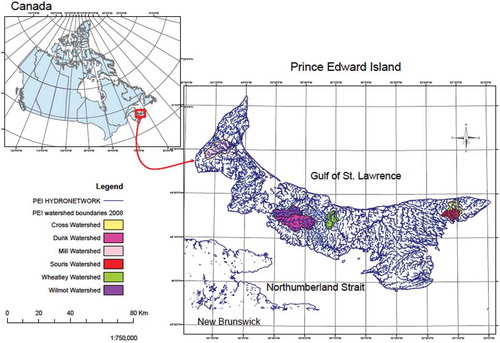
2.1 Study watersheds

Six drainage basins located in Prince Edward Island, Canada, were selected for the present study: the Wilmot, Dunk, Mill, Cross, Wheatley and Souris river basins (see Fig. 1). The distribution of percentage surface area occupied by agriculture and forest (PEI Department of Environment/Energy & Forestry and Resource Inventory 2010) for those watersheds is presented in Table 1. The dominant soil types for each watershed have been identified, as well as their respective percentages of drainage area (see Table 1). All the soil types of the studied watersheds have mainly a fine sandy loam texture. They include the Charlottetown soil type, which is mainly well drained, the Cullodon, Tignish, O’Leary and Albery soil types with moderate drainage, and the Malpeque and Duvar soil types, which are poorly drained (Research Branch Agriculture Canada/PEI Department of Agriculture 1994). Geologically, the sedimentary materials of PEI are referred to as Permo-Carboniferous rocks and are dominated by red-coloured sandstone and mudstone (Van De Poll 1989).

Table 1. Land use and soil types for the study watersheds.

	Cross River	Souris River	Wheatley River	Dunk River	Wilmot River	Mill River
Station coordinates
Latitude	46°27ʹ38″	46°23ʹ27″	46°21ʹ50″	46°20ʹ51″	46°26ʹ39″	46°44ʹ39″
Longitudinal	62°16ʹ4″	62°18ʹ26″	63°17ʹ17″	63°39ʹ46″	63°39ʹ44″	64°11ʹ2″
Area (km^2)	37.67	14.41	21.13	140.6	48.94	48.98
Land use (%)
Agriculture	10.2	29.7	68.9	66.2	81.7	31.3
Forest	83.0	60.8	20.4	25.2	10.1	57.0
Others	6.8	9.5	10.7	8.60	8.20	11.7
Soil type (%)
Charlottetown	29.8	14.3	81.2	74.0	79.7	9.10
Albery	43.6	53.7	12.9	17.7	8.10
Malpeque	2.30				6.20
Cullodon	8.20	15.1
Winsloe	4.40
Tignish						6.60
Margate						33.3
O Leary						23.9
Duvar						14.9

Figure 1. Locations and boundaries of the study watersheds on Prince Edward Island, Canada.

2.2 Turbidity data collection

Turbidity measurements in rivers were performed using two types of turbidity probes (see Table 2). Turbidity loggers were deployed from 8 December 2012 to 31 August 2015. Turbidity sensors measure the turbidity of water using infrared radiation transmitted and reflected by the suspended sediments. Sensors were calibrated first with turbidity standards and the sampling frequency was set at 30 min, with an automatic wiper cleaning every 24 h, prior to sampling.

Table 2. Meteorological and hydrometric stations used in this study.

River	Turbidity sensors	Hydrometric station	Station ID	Meteorological station	Climatic ID
Cross	Eureka 2			St Peters	8300562
Wilmot	YSI 6136	Wilmot River near Wilmot Valley	01CB004	New Glasgow	8300497
				Elmwood	8300425
Souris	Eureka 2			Alliston	8300100
Mill	YSI 6136	Carruthers Brook near St-Anthony	01CA003	Alberton Snow	8300085
				Tyne Valley	8300846
Dunk	YSI 6136	Dunk River at Wall Road	01CB002	Elmwood	8300425
				New Glasgow	8300497
Wheatley	Eureka 2			Summerside	8300596

The relationship between the turbidity and SSC was determined for every river with the calibration curve established using the method of Pavey et al. (2007). The calibration curve for each turbidity probe was performed using mixtures of in situ water and local sediment with particles of maximum size 63 micrometres. Thus, different ratios of water and sediments were continuously stirred in a 40-L tank and the value of the turbidity was recorded in conjunction with the collection of a 500-mL grab sample, which was subsequently, filtered, dried and weighed in the laboratory. A nonlinear mathematical relationship between SSC and turbidity was chosen for all monitoring sites after analysis of graphs. The equation form that was used for the relationship is:

(1)

where C is the suspended sediment concentration; T is the water turbidity; and a and b are the coefficients estimated through fitting using a routine based on the Levenberg-Marquardt algorithm, which is a variant of the Gauss-Newton iterative method. The method minimizes the sum of the squares of the residuals and has been shown to provide a better approximation compared to the ordinary least square method (St‐Hilaire et al. 2005).

2.3 Meteorological and hydrometric data

Precipitation and surface runoff have a major influence on soil erosion over land and flow plays an important role in the transport capacity of suspended sediment within a river. Daily precipitation data from weather stations operated by Environment Canada (http://climate.weather.gc.ca) and located nearest each site were used (Table 2). The daily streamflow data were obtained from Environment Canada (Water Survey Division) from hydrometric stations (http://wateroffice.ec.gc.ca) described in Table 2.

For the Cross, Souris and Wheatley rivers, which are not currently gauged by Environment Canada, water-level loggers were installed adjacent to the turbidity logging stations. Water levels were recorded at 30-min time step with ONSET HOBO water-level loggers installed at the bottom and top of a stilling well. According to standard set-up, the top-level logger was measuring atmospheric pressure, in order to subtract that pressure from the values recorded by the bottom logger, which was reading total (i.e. atmospheric and hydrostatic) pressures, ultimately converted to levels. Spot-discharge measurements were taken using a Marsh McBirney velocity meter in order to construct stage–discharge rating curves for these three rivers.

To test surface runoff (in contrast with total discharge, which combines baseflow and surface runoff) as a predictor, hydrograph separation was performed using the Web-based Hydrograph Analysis Tool (WHAT; Lim et al. 2005). The WHAT system uses the general form of a digital filtering proposed by Eckhardt (2005) to separate baseflow from total daily streamflow. For all studied rivers, a value equal to 0.8 for the BFImax (maximum value of long-term ratio of baseflow to total streamflow) was used, as recommended by Eckhardt (2005) for perennial streams with porous aquifers.

2.4 Adaptive neuro-fuzzy inference system methods

The ANFIS-based models take advantage of the learning capacity of artificial neural networks and the ability of fuzzy logic to express knowledge about a system using standard linguistic rules, namely by combining input categories and the result of the combinations using IF…THEN sentences. ANFIS also re-injects actual numerical input data in the model as weighted sums to modulate its output (Takagi and Sugeno 1985). An example of the ANFIS architecture for two input variables x1 and x2 is shown in Figure 2. The fuzzy rules for this example can be stated as follows:

(2)

Figure 2. Architecture of an ANFIS model (adapted from Jang 1993).

where p_i, q_i and r_i are consequent parameters that can be estimated by using the ordinary least squares method, and B_i and A_i are linguistic values defined by fuzzy sets.

In Figure 2, the fuzzification layer (Layer 1) associates a membership function with each node that defines the degree of compatibility with category (e.g. high flow) represented by a fuzzy set (Godjevac 1999). A membership function of a fuzzy set, as proposed by Zadeh (1965), is a generalization of the indicator function in classical sets with a range covering the interval [0,1]. Fuzzy sets can be constructed using various simple linear or nonlinear functions. For instance, for a generalized bell-shaped membership function, the output of the ith node of layer 1 () is given by:

(3)

where is the membership degree of (varying between 0 for a value excluded from the membership to 1 for a value that fully belongs to the category defined by the fuzzy set); and a_i, b_i and c_i are premise parameters. The parameter a_i corresponds to the membership function centre, while b_i and c_i determine the slopes at the inflection points of the function used to define the fuzzy set.

In Layer 2 shown in Figure 2, each node performs a fuzzy T-standard that defines the class of intersection operators for fuzzy subsets (Godjevac 1999). The output of Layer 2 nodes is obtained from:

(4)

where and are membership degrees for input variables x1 and x2, respectively.

The outputs of the T-standards are standardized in Layer 3. The output of Layer 3 nodes in the example is obtained using the relationship:

(5)

In Layer 4, a linear combination of input variables is applied. The output of the Layer 4 nodes () is obtained from:

(6)

where p_i, q_i and r_i are conclusion parameters that can be estimated using the least squares method for input variables x1 and x2.

Finally, the predicted output of Layer 5 () is obtained by a weighted mean of Layer 4 outputs:

(7)

To train fuzzy systems, the ANFIS hybrid algorithm uses first the least square estimator to adjust the consequent parameters according to premise parameters. Second, it uses the gradient descent algorithm to adjust the premise parameters according to the consequent parameters by adapting the connection weights to minimize errors.

The database used was split into two subsets: two-thirds were used for the model calibration (the so-called learning phase) and the remainder for model validation. The GENFIS1 and EVALFIS functions in Matlab’s fuzzy logic toolbox (MathWorks 2015) were used, respectively, to design a fuzzy inference system structure for ANFIS training and to perform fuzzy inference calculations. Thus, the number and type of membership functions were determined experimentally, by developing various models and studying their results. The performance criteria for the model were then calculated in both the calibration and validation phases. Three of the most commonly recommended criteria, namely the Nash-Sutcliffe coefficient (NS, Nash and Sutcliffe 1970, Moriasi et al. 2007), the root mean square error (RMSE) and the bias were used for model assessment.

2.5 Development of watershed vulnerability index

The watershed vulnerability index, a variable introduced as a supplement to the other ANFIS model inputs, aims to take into account the impact of factors related to soil vulnerability to water erosion. Factors related to soil characteristics, topographic basins and land-use and management practice play a major role in the sediment reaching the river. The mean slopes of the studied watersheds were low and were all of the same order of magnitude. The most dynamic variables typically used in empirical models, such as the universal soil loss equation (USLE) developed by the US Department of Agriculture in the 1950s (Wischmeier et al. 1958, Wischmeier 1959), were included. They are the soil erodibility factor K, with crops and management factor C. The USLE also includes a support and management practice factor P, which represents the soil loss associated with an agricultural support and management practice other than traditional straight-row ploughing parallel to the land slope. There were no data available that would allow for the inclusion of the practice factor (e.g. information on contouring, terracing and strip cropping) in the model, and it was set to 1 for the studied watersheds. The topographic data were also excluded as a model input because the mean slopes of the studied watersheds were low and were very similar among the studied drainage basins. A watershed vulnerability index K_r was developed and calculated for each watershed using only soil erodibility K with crops and management factor C. The advantage of combining these two variables is to integrate into the ANFIS-based model the variable that takes into account the spatio-temporal distribution of the soil sensitivity or soil vulnerability to water erosion, depending on land use. The parameters that affect the K factor are soil texture, organic matter content, soil structure, permeability and seasonal fluctuations (Wall et al. 2002). The formula proposed by Williams and Singh (1995) was used to calculate the soil erodibility factor K:

where , and are, respectively, the percentages of silt, sand and organic matter.

The PEI soil layers were used to identify different types of soils in every watershed and the soil erodibility factor K for every type of soil was calculated using information on physical properties (size distribution and organic matter) given by the Canadian Soil Information Service (http://sis.agr.gc.ca/siscan). A weighted mean of K values was computed for every basin according to the proportion of surface area occupied by different types of soils. To better account for the seasonal fluctuations in the soil erodibility factor:

• monthly distributions of the rainfall erosivity index from the climatic station closest to the site were extracted from the RUSLE-CAN manual (Wall et al. 2002);

• monthly K values were weighted according to the distribution of erosive rainfall throughout the year; and

• monthly K values were multiplied by a factor of 2 during the winter–spring thaw period, as recommended by Wall et al. (1988).

Calculating the crops and management factor C requires data about crop canopy, surface cover, soil biomass, tillage, surface roughness, prior land use and the distribution of erosive rainfall (Wall et al. 2002). The C values for periods corresponding to five crop stages for every year proposed by Wischemieir and Smith (1965) were used. For every watershed, a weighted mean of C values for different crop stages was calculated according to the distribution of surface area occupied by different types of crops at different stages. Monthly C values were subsequently weighted according to the proportion of erosive rainfall index from the nearest climatic station. The monthly values of the watershed vulnerability index were obtained by combining both factors (the monthly C values and monthly K values) and multiplying by the surface area of each watershed to account for the impact of the contributing area. Daily values of watershed vulnerability index were smoothed/interpolated from monthly values using the piecewise cubic Hermite interpolation method (Fritsch and Carlson 1980).

3 Results and discussion

3.1 Watershed vulnerability index and sediment monitoring results

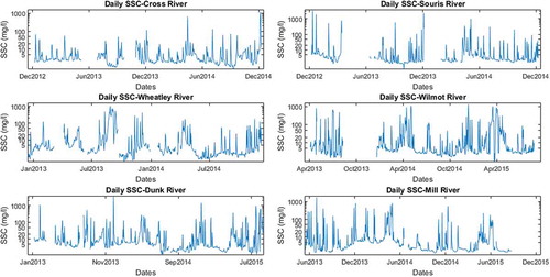
The SSC data used in this study were obtained using mathematical relationships developed using the calibration curves. The parameters of the equation used to calculate SSC vs turbidity are presented in Table 3 alongside four performance criteria (RMSE, NS coefficient, R² and bias), and an example of a calibration curve is shown in Figure 3 for the Wilmot River. The final results of suspended sediment monitoring for all studied watersheds are shown in Figure 4.

Table 3. Values of parameters for all rivers in the equation: SSC = a[turbidity]^b.

River	Parameter a	Parameter b	NS	RMSE (mg/L)	R^2	Bias (10^–2)
Cross	1.61	0.96	0.99	8.8	0.99	0.15
Wilmot	0.97	1.19	0.98	99.2	0.98	–1.28
Souris	2.33	0.88	0.99	16.1	0.99	0.80
Mill	0.08	1.64	0.95	529.2	0.95	−3.5
Dunk	0.06	1.52	0.94	257.8	0.94	–9.0
Wheatley	1.48	0.98	0.99	83.4	0.98	–0.03

Figure 3. Calibration curve for the Wilmot River.

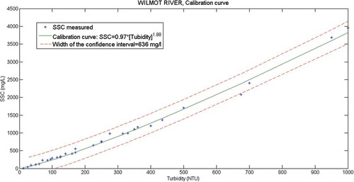
Figure 4. Times series of daily SSC on the six rivers monitored in this study.

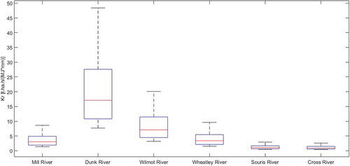
Examples of mean monthly SSC vs mean monthly watershed vulnerability index for January–November 2014 and the box plot of the watershed vulnerability index for each watershed are shown in Figures 5 and 6, respectively. Analysing the graph of Figure 5 shows that the maximum watershed vulnerability index value is observed during freezing and thawing periods, while it becomes moderately high at planting time and tends to be low at crop maturity. The shape of the time series in Figure 5 shows that there is a strong relationship between the seasonal variation of the watershed vulnerability index and SSC. Thus the watershed vulnerability index seems to show an influence on the temporal variability of SSC for the studied watersheds. Figure 6 shows that the Dunk River has the highest value of watershed vulnerability index K_r corresponding to a relatively high percentage of agriculture (66%). The Wilmot River also has high agricultural land cover (8% of drainage area) and has similar K_r values as the Wheatley River, which has 70% of its drainage area used for agriculture. Comparing the C (crop and management factor) component of watershed vulnerability index between different watersheds, it was found that this factor has the greatest influence on the index K_r, with a coefficient of variation of 50% between watersheds. The averaged soil erodibility factor K showed much lower variability between the six watersheds, with a coefficient of variation of 3.5%. When month is accounted for, there were no significant differences in K_r between the Wilmot, Wheatley, Souris and Cross watersheds. Also, scaling the averaged watershed vulnerability index using the drainage area was a first attempt at representing the scale of sediment supplies on the ground. The net result is that basins with up to 60% of their drainage area used for agriculture (i.e. the Dunk, Wilmot and Wheatley river basins) are the ones with the highest values of watershed vulnerability index.

Figure 5. Hydrographs of mean monthly SSC vs watershed vulnerability index.

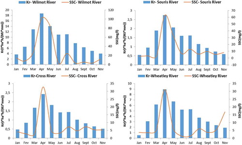
Figure 6. Box plot of watershed vulnerability index for the studied watersheds.

3.2 ANFIS models results for each watershed

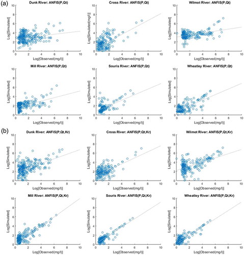
Various ANFIS models were developed and their results were studied for different combinations of input data: i.e. precipitation (P), total discharge (Q), surface runoff (q_R) and watershed vulnerability index (K_r). The first two-thirds of the data were used for calibration and the last third for validation. The model performance indicators obtained using different combinations of input variables in the ANFIS for the six watersheds are presented in Table 4. Scatter plots of observed vs simulated SSC for ANFIS models with various combinations of input variables for the validation phase are shown in Figure 7(a) and (b). The best performance was obtained when precipitation, total flow and watershed vulnerability index were used as input variables. This result demonstrates the roles played by total flow and the source of sediments, respectively, in the transport capacity of suspended sediment within the water column of a river and in the spatiotemporal variation of sediment budgets depending on watershed characteristics (land use, soil erodibility, etc.) under the meteorological constraints.

Table 4. Performance of river-specific models using total flow (Q_t), precipitation (P), surface runoff (q_R), and watershed vulnerability index (K_r).

River	Input variables	Training data			Validation data
		NS	RMSE (mg/L)	Bias (10^–2)	NS	RMSE (mg/L)	Bias (10^–2)
Cross	P, Qt	0.86	6.7	0.49	0.56	28.6	−0.59
	P, qR	0.92	5.0	−0.42	0.58	27.9	2.4
	P, Qt, Kr	0.95	4.5	−0.48	0.83	14.2	0.45
	P, qR, Kr	0.94	3.9	0.19	0.79	19.53	0.44
Wilmot	P, Qt	0.68	33.9	−1.2	0.52	105.3	0.24
	P, qR	0.71	31.9	−1.0	0.66	88.4	0.18
	P, Qt, Kr	0.75	56.8	0.6	0.71	70.1	−0.20
	P, qR, Kr	0.73	48.7	−0.5	0.62	75.8	0.48
Souris	P, Qt	0.74	20.9	−0.47	0.67	6.7	0.07
	P, qR	0.79	18.5	−2.02	0.74	5.9	5.00
	P, Qt, Kr	0.84	16.6	−0.07	0.86	4.30	0.30
	P, qR, Kr	0.78	19.41	0.2	0.82	4.9	0.02
Mill	P, Qt	0.63	50.10	−0.25	0.69	25.2	−2.80
	P, qR	0.61	55.35	0.17	0.65	26.4	−0.04
	P, Qt, Kr	0.72	37.16	−0.9	0.80	21.9	0.19
	P, qR, Kr	0.75	28.5	−0.31	0.77	23.4	−2.71
Wheatley	P, Qt	0.85	26.8	0.22	0.77	43.7	2.40
	P, qR	0.86	22.7	−0.03	0.80	33.6	−2.41
	P, Qt, Kr	0.86	20.0	0.6	0.82	30.4	0.20
	P, qR, Kr	0.86	29.8	−0.41	0.81	34.85	0.15
Dunk	P, Qt	0.36	98.3	0.73	0.34	103.3	0.80
	P, qR	0.37	96.0	−0.72	0.39	92.2	0.83
	P, Qt, Kr	0.57	68.4	0.31	0.55	79.5	−0.05
	P, qR, Kr	0.55	87.5	−0.14	0.53	86.9	0.08

Figure 7. Scatter plots of observed vs computed SSC (validation phase) for input variables (a) P and Q_t, and (b) P, Q_t and K_r.

3.3 Multi-watershed ANFIS model results

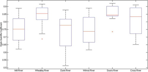
Random subsamples of the datasets (the first two-thirds of data) from each watershed were combined together in order to train the ANFIS and develop a global model which can be applied to any of the six rivers. The remaining data were used for validation of the multi-watershed ANFIS model. Only total flow, precipitation and K_r values were used as input variables, as this combination of inputs provided the best results for river-specific models. The performance indicators for the multi-watershed model are presented in Table 5. Figure 8 presents simulated versus observed SSC in the validation phase. When comparing the multi-watershed ANFIS versus single-watershed ANFIS model results in validation phase, it can be seen that the NS coefficients were decreased by 1.20% for the Cross River, 3.48% for the Souris River, and 1.22% for the Wheatley River, while they were increased by 9.09% for the Dunk River, 7.04% for the Wilmot River and 1.25% for the Mill River. Finally, the stability of multi-watershed ANFIS models was tested. Given that subsamples of input data from each watershed must be used to train the model, the experience needed to be repeated a number of times for varying training datasets. Model training was repeated 20 times using different randomly selected subsamples from all studied watersheds. Results show the highest and lowest inter-quartile ranges for the NS coefficient for the Dunk River and the Souris River, respectively (Fig. 9). All median NS coefficient values were above 0.7 and no NS coefficient value was below 0.5.

Table 5. Performance of the multi-watershed ANFIS model.

River	Input Variables	Training data			Validation data
		NS	RMSE (mg/L)	Bias (10^–2)	NS	RMSE (mg/L)	Bias (10^–2)
Cross	P, Qt, Kr	0.85	33.90	–3.28	0.82	17.55	–1.49
Wilmot	P, Qt, Kr	0.85	33.89	–1.64	0.76	53.8	–0.16
Souris	P, Qt, Kr	0.85	33.89	–2.35	0.83	4.35	–0.8
Mill	P, Qt, Kr	0.85	33.93	0.53	0.81	20.93	–2.03
Dunk	P, Qt, Kr	0.85	33.91	–1.27	0.61	65.6	7.21
Wheatley	P, Qt, Kr	0.85	33.92	2.10	0.81	31.26	4.19

Figure 8. Scatter plots of simulated vs observed SSC for the multi-watershed ANFIS model.

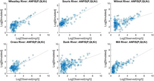
Figure 9. Boxplot of NS coefficient values obtained using 20 different random subsamples of input data to train the multi-watershed ANFIS model.

4 Conclusion

In the present study, a data-driven model based on the ANFIS approach was evaluated for estimating suspended sediment concentrations in rivers of six agriculture-dominated watersheds of Prince Edward Island, Canada. Different combinations of inputs were tested including precipitation, surface runoff rate, total flow and a parameter that accounts for the temporal variability of soil erodibility according to soil and crop types. The introduction of the erosion vulnerability index significantly improved the ability of the ANFIS model to estimate SSC within the watershed. To the knowledge for the authors, this is the first attempt at including such an input to a data-driven model for SSC estimations in agricultural watersheds.

In previous studies, even when used without inputs describing the erodibility of the drainage basin, the neuro-fuzzy modelling had shown potential to become a powerful tool for estimating SSC compared to other data-driven models (Kisi 2005, Kisi et al. 2009, Rajaee et al. 2009, Salajegheh et al. 2011, Seyedian and Rouhani 2015). For examples, Kisi (2005) applied an ANFIS model for daily suspended sediment estimation from flow data for the Quebrada Blanca River and the Rio Valenciano River (USA) and the results indicated that the ANFIS model provides higher accuracy and reliability than the artificial neural networks, the multi-linear regression and the SRC models. The ANFIS model had the smallest RMSE and highest R², equal to 2.72 mg/L and 0.876, respectively, for the Rion Valenciano River, while for the Quebrada Blanca River, the values were, respectively, 0.94 mg/L and 0.929. In another case study, the better performance of ANFIS compared to SRC results was also reported by Kisi et al. (2009) for monthly suspended sediment prediction using flow in Turkey (Kylus and Salur Koprusu stations in Kizilirmak Basin). The minimum RMSE and highest R² were, respectively, 1970 t and 0.785 for Kylus station, and 39.416 t and 0.76 for Salur Koprusu station. The capabilities offered by ANFIS were also explored in comparison with the SRC model to estimate daily SSC using flow data by Seyedian and Rouhani (2015) at four stations in the USA (Merrimack River at Alowell, Choptank near Greensboro, Susquehanna River at Harrisburg and Swatara Creek at Harper Tavern). Their results showed that the accuracy of the ANFIS model was more acceptable than that of the SRC model, with R² ranging from 0.23 to 0.95 and RMSE in the range 3.6–7506 mg/L.

Furthermore, this study showed the potential of implementing such a model on multiple watersheds. The multi-watershed model results were deemed adequate when compared to the same model trained on individual rivers. The multi-watershed ANFIS model performance varied with different training sets, but never lost its predictive capacity (NS > 0.5), which again indicates that the approach has the potential to be used on a regional scale, provided that subsamples of inputs used for the training sets encompass most conditions occurring on individual watersheds. This study opens the door to further investigations; additional work will be needed to see how the spatial variation of the index within a watershed can affect SSC and to revisit the need for scaling the ind ex by drainage area.

Acknowledgements

We would like to thank Christina Pater for her help during field work.

Disclosure statement

No potential conflict of interest was reported by the authors.

Additional information

Funding

The authors wish to acknowledge funding received from the Canadian Water Network for this work.

References

- Abrahart, R.J., et al., 2011. DAMP: A protocol for contextualising goodness-of-fit statistics in sediment-discharge data-driven modelling. Journal of Hydrology, 409 (3–4), 596–611. doi:10.1016/j.jhydrol.2011.08.054
- Ashmore, P., et al., 2000. Recent (1995–1998) Canadian research on contemporary processes of river erosion and sedimentation, and river mechanics. Hydrological Processes, 14 (9), 1687–1706. doi:10.1002/(ISSN)1099-1085
- Aytek, A. and Kişi, Ö., 2008. A genetic programming approach to suspended sediment modelling. Journal of Hydrology, 351 (3–4), 288–298. doi:10.1016/j.jhydrol.2007.12.005
- Buck, O., Niyogi, D.K., and Townsend, C.R., 2004. Scale-dependence of land use effects on water quality of streams in agricultural catchments. Environmental Pollution, 130 (2), 287–299. doi:10.1016/j.envpol.2003.10.018
- Cairns, D.K., 2001. An evaluation of possible causes of decline in pre-fisheries abundance of North American Atlantic Salmon. Canadian Techical Reports Fisheries and Aquatic Sciences, 2358, 67.
- Collins, A.L. and Walling, D.E., 2004. Documenting catchment suspended sediment sources: problems, approaches and prospects. Progress in Physical Geography, 28 (2), 159–196. doi:10.1191/0309133304pp409ra
- Commission on Land and Local Governance, 2009. Report of Commission on Land and Local Governance. Communications PEI-Document Publishing Centre, Charlottetown. 163 p
- Dong, J., Xia, X., and Zhai, Y., 2013. Investigating particle concentration effects of polycyclic aromatic hydrocarbon (PAH) sorption on sediment considering the freely dissolved concentrations of PAHs. Journal of Soils and Sediments, 13 (8), 1469–1477. doi:10.1007/s11368-013-0736-9
- Downing, J., 2005. Environmental Instrumentation and Analysis Handbook. Chapitre 24: turbidity monitoring. John Wiley and Sons, 270, 511–546.
- Eckhardt, K., 2005. How to construct recursive digital filters for baseflow separation. Hydrological Processes, 19 (2), 507–515. doi:10.1002/(ISSN)1099-1085
- Fritsch, F.N. and Carlson, R.E., 1980. Monotone Piecewise Cubic Interpolation. SIAM Journal on Numerical Analysis, 17 (2), 238–246. doi:10.1137/0717021
- Gao, P., 2008. Understanding watershed suspended sediment transport. Progress in Physical Geography, 32 (3), 243–263. doi:10.1177/0309133308094849
- Gippel, C.J., 1995. Potential of turbidity monitoring for measuring the transport of suspended solids in streams. Hydrological Processes, 9 (1), 83–97. doi:10.1002/(ISSN)1099-1085
- Godjevac, J.É., 1999. Idées nettes sur la logique floue. 1st éd ed. Lausanne: Presses Polytechniques et Universitaires Romandes, 128.
- Higgins, H., et al., 2011. Suspended sediment dynamics in a tributary of the Saint John River, New Brunswick. Canadian Journal of Civil Engineering, 38 (2), 221–232. doi:10.1139/L10-129
- Horowitz, A.J., 2003. An evaluation of sediment rating curves for estimating suspended sediment concentrations for subsequent flux calculations. Hydrological Processes, 17 (17), 3387–3409. doi:10.1002/(ISSN)1099-1085
- Jang, J.S.R., 1993. ANFIS: adaptive-network-based fuzzy inference system. IEEE Transactions on Systems, Man, and Cybernetics, 23 (3), 665–685. doi:10.1109/21.256541
- Kachanoski, R.G., 1992. Evaluation of soil loss rates under different soil and cropping practices in Prince Edward Island. Guelph, ON: University of Guelph.
- Kachanoski, R.G. and Carter, M.R., 1999. Landscape position and soil redistribution under three soil types and land use practices in Prince Edward Island. Soil and Tillage Research, 51 (3–4), 211–217. doi:10.1016/S0167-1987(99)00038-0
- Kisi, O., 2005. Suspended sediment estimation using neuro-fuzzy and neural network approaches/Estimation des matières en suspension par des approches neurofloues et à base de réseau de neurones. Hydrological Sciences Journal, 50 (4). doi:10.1623/hysj.2005.50.4.683
- Kisi, O., et al., 2009. Adaptive neuro-fuzzy computing technique for suspended sediment estimation. Advances in Engineering Software, 40 (6), 438–444. doi:10.1016/j.advengsoft.2008.06.004
- Kisi, O., 2016. A new approach for modeling suspended sediment: evolutionary fuzzy approach. Hydrology and Earth Systems Sciences Discussions, 2016, 1–41. doi:10.5194/hess-2016-213
- Li, H., Liu, L., and Ji, X., 2015. Modeling the relationship between landscape characteristics and water quality in a typical highly intensive agricultural small watershed, Dongting lake basin, south central China. Environmental Monitoring and Assessment, 187 (3), 129. doi:10.1007/s10661-015-4349-1
- Lim, K.J., et al., 2005. Automated Web GIS Based Hydrograph Analysis Tool, WHAT. Journal of the American Water Resources Association, 41 (6), 1407–1416. doi:10.1111/jawr.2005.41.issue-6
- Lisle, T.E. and Lewis, J., 1992. Effects of sediment transport on survival of salmonid embryos in a natural stream: a simulation approach. Canadian Journal of Fisheries and Aquatic Sciences, 49 (11), 2337–2344. doi:10.1139/f92-257
- MathWorks, I., 2015. Matlab: Fuzzy Logic Toolbox. R2015a. Natick, MA: MathWorks,Inc.
- Merritt, W. S., Letcher, R. A., and Jakeman, A. J., 2003. A review of erosion and sediment transport models. Environmental Modelling & Software, 18 (8), 761–799. doi:10.1016/S1364-8152(03)00078-1
- Minella, J.P., et al., 2008. Estimating suspended sediment concentrations from turbidity measurements and the calibration problem. Hydrological Processes, 22 (12), 1819–1830. doi:10.1002/hyp.6763
- Moriasi, D., et al., 2007. Model evaluation guidelines for systematic quantification of accuracy in watershed simulations. Transactions of the ASABE, 50 (3), 885–900. doi:10.13031/2013.23153
- Nash, J. and Sutcliffe, J.V., 1970. River flow forecasting through conceptual models part I—A discussion of principles. Journal of Hydrology, 10 (3), 282–290. doi:10.1016/0022-1694(70)90255-6
- Ouellet-Proulx, S., et al., 2015. Estimation of suspended sediment concentration in the Saint John River using rating curves and a machine learning approach. Hydrological Sciences Journal, Published online. doi:10.1080/02626667.2015.1051982
- Pavey, B., et al., 2007. Exploratory study of suspended sediment concentrations downstream of harvested peat bogs. Environmental Monitoring and Assessment, 135 (1–3), 369–382. doi:10.1007/s10661-007-9656-8
- PEI Department of Environment/Energy & Forestry and Resource Inventory, 2010. Corporated Land Use Inventory 2010. Available from: www.gov.pe.ca/gis.
- Prince Edward Island Department of Fisheries and Environment, 1996. Water on Prince Edward Island: understanding the resource, knowing the issues. Montague: Prince Edward Island Department of Fisheries and Environment.
- Rajaee, T., et al., 2009. Daily suspended sediment concentration simulation using ANN and neuro-fuzzy models. Science of the Total Environment, 407 (17), 4916–4927. doi:10.1016/j.scitotenv.2009.05.016
- Research Branch Agriculture Canada/PEI Department of Agriculture, 1994. Soil Survey of PEI. Available from: www.gov.pe.ca/gis.
- Sadar, M., 2002. Turbidity instrumentation–an overview of today’s available technology. Turbidity and Other Sediment Surrogates Workshop, Nevada, 62.
- Salajegheh, A., et al., 2011 Investigation of the multi layer perceptron, fuzzy logic and neuro-fuzzy for estimating of suspended load. International Conference on Chemical, Biological and Environment Sciences. ( Bangkok, December), p 444–449.
- Seyedian, S. and Rouhani, H., 2015. Assessing ANFIS accuracy in estimation of suspended sediments. Građevinar, 67 (12). doi:10.14256/JCE.1210.2015
- St‐Hilaire, A., et al., 2005. Streambed sediment composition and deposition in a forested stream: spatial and temporal analysis. River Research and Applications, 21 (8), 883–898. doi:10.1002/(ISSN)1535-1467
- Stonehouse, D.P. and Bohl, M., 1990. Land degradation issues in Canadian agriculture. Canadian Public Policy /Analyse De Politiques, 16 (4), 418–431. doi:10.2307/3550856
- Takagi, T. and Sugeno, M., 1985. Fuzzy identification of systems and its applications to modeling and control. IEEE Transactions on Systems, Man, and Cybernetics, SMC-15 (1), 116–132. doi:10.1109/TSMC.1985.6313399
- Tramblay, Y., St-Hilaire, A., and Ouarda, T.B.M.J., 2008. Frequency analysis of maximum annual suspended sediment concentrations in North America /Analyse fréquentielle des maximums annuels de concentration en sédiments en suspension en Amérique du Nord. Hydrological Sciences Journal, 53 (1), 236–252. doi:10.1623/hysj.53.1.236
- USEPA (US Environmental Protection Agency)., 1996. Nonpoint source pollution: the Nation’s largest water quality problem. Pointer No. 1, EPA841-F-96-004A. Available from: http://water.epa.gov/polwaste/nps/outreach/point1.cfm [ Accessed 20 Nov 2015].
- van de Poll, H.W., 1989. Lithostratigraphy of the Prince Edward Island redbeds. Atlantic Geology, [S.l.], apr. 1989. ISSN 1718-7885. Available from: https://journals.lib.unb.ca/index.php/ag/article/view/1668 [ Accessed 11 Dec 2016]
- Wall, G.J., et al., 1988. Seasonal soil erodibility variation in southwestern ontario. Canadian Journal of Soil Science, 68 (2), 417–424. doi:10.4141/cjss88-038
- Wall, G.J., et al., 1995. Erosion. Ottawa: The health of our soils-toward sustainable agriculture in Canada. Centre for Land and Biological Resources Research, Research Branch, Agriculture and Agri-Food Canada, 61–67. Ont:3.
- Wall, G.J., et al., 2002. RUSLE-CAN — Équation universelle révisée des pertes de sol pour application au Canada. Manuel pour l’évaluation des pertes de sol causées par l’érosion hydrique au Canada. Direction générale de la recherche, Agriculture et Agroalimentaire Canada, Ottawa (Ontario), No de la contribution AAC2244F, 117p.
- Williams, J.R., 1995. The EPIC model. In: V.P. Singh, ed. Computer models of watershed hydrology. Highlands Ranch, CO: Water Resources Publications, 909–1000.
- Wischmeier, W.H., 1959. A rainfall erosion index for a universal soil loss equation. Soil Science Society of America Journal, 23 (3), 246–249. doi:10.2136/sssaj1959.03615995002300030027x
- Wischmeier, W.H., Smith, D., and Uhland, R.E., 1958. Evaluation of factors in the soil loss equation. Agricultural Engineering, 36, 458–462.
- Wischmeier, W.H. and Smith, D.D., 1965. Predicting rainfall-erosion losses from cropland east of the Rocky Mountains-guide for selection of practices for soil and water conservation. Washington, DC: U.S. Department of Agriculture, Agriculture Handbook No. 282.
- Wölz, J., et al., 2010. Impact of contaminants bound to suspended particulate matter in the context of flood events. Journal of Soils and Sediments, 10 (6), 1174–1185. doi:10.1007/s11368-010-0262-y
- Wood, P.J. and Armitage, P.D., 1997. Biological effects of fine sediment in the lotic environment. Environmental Management, 21 (2), 203–217. doi:10.1007/s002679900019
- Xia, X., et al., 2016. Effect of water-sediment regulation of the Xiaolangdi reservoir on the concentrations, characteristics, and fluxes of suspended sediment and organic carbon in the Yellow River. Science of the Total Environment, 571, 487–497. doi:10.1016/j.scitotenv.2016.07.015
- Zadeh, L.A., 1965. Fuzzy sets. Information and Control, 8 (3), 338–353. doi:10.1016/S0019-9958(65)90241-X
- Zhang, X., et al., 2015. Bioavailability of pyrene associated with suspended sediment of different grain sizes to daphnia magna as investigated by passive dosing devices. Environmental Science & Technology, 49 (16), 10127–10135. doi:10.1021/acs.est.5b02045