Simple vs complex rating curves: accounting for measurement uncertainty, slope ratio and sample size

ABSTRACT

Multiple segmented rating curves have been proposed to better capture the variability of the physical and hydraulic characteristics of river–floodplain systems. We evaluate the accuracy of one- and two-segmented rating curves by exploiting a large and unique database of direct measurements of stage and discharge data in more than 200 Swedish catchments. Such a comparison is made by explicitly accounting for the potential impact of measurement uncertainty. This study shows that two-segmented rating curves did not fit the data significantly better, nor did they generate fewer errors than one-segmented rating curves. Two-segmented rating curves were found to be slightly beneficial for low flow when there were strong indications of segmentation, but predicted the rating relationship worse in cases of weak indication of segmentation. Other factors were found to have a larger impact on rating curve errors, such as the uncertainty of the discharge measurements and the type of regression method.

KEYWORDS:

• rating curve
• river discharge
• gauging station
• uncertainty
• overfitting
• validation

EDITOR M.C. Acreman; ASSOCIATE EDITOR not assigned

1 Introduction

1.1 Premise and aim of this study

Water resources management, flood risk assessment, drought and water scarcity studies, and hydrological and hydraulic modelling rely strongly on the quality of streamflow data (McMillan et al. 2012, Strömqvist et al. 2012, Westerberg et al. 2016). Gauging stations usually only record the water stage, h, which is then translated into river discharge, Q, by means of a stage–discharge relationship. This relationship, hereafter referred to as the rating curve, is derived by parameterizing simple functions using a number of direct measurements of discharge at different stage values (Herschy 1999, WMO 2008). The accuracy of rating curves is of great interest for hydrologists because observation errors will propagate to hydrological models or studies based on these data (Lang et al. 2010, Domeneghetti et al. 2012, Haque et al. 2014).

A single power function is often used to derive rating curves because of its resemblance to the Manning equation (Petersen-Overleir 2009) and the relatively low number of parameters (Herschy 1999, Di Baldassarre and Claps 2011). More complex approaches can be based on the use of multiple segments of power law functions (Reitan and Petersen-Overleir 2009). Segmentation is believed to better capture changes in river geometry and friction for different water stages, e.g. transition into floodplain (Lambie 1978, Herschy 1999). Yet, the potential and limitations of using multi-segmented rating curves have not been extensively explored. One of the main issues in building rating curves is that direct measurements of discharge are often very limited. Consequently, using multi-segmented curves (requiring the estimation of more than five parameters) instead of traditional one-segmented curves can lead to overfitting, i.e. fitting the noise instead of the signal in the data.

Here we compare one-segmented and two-segmented rating curves in terms of calibration, interpolation and extrapolation errors. This comparison is made by using a large database of Swedish stage–discharge measurements from over 200 gauging stations. Also, we run Monte Carlo simulations to explore the potential role of uncertainty associated with these direct measurements.

1.2 Background: power function

Direct discharge measurements are rare mainly because they rely on expensive equipment. These measurements are even rarer during extreme events because of high water velocities, danger for staff and equipment, operational timing and changes in the cross-sections due to e.g. erosion (Petersen-Overleir and Reitan 2005).

Many countries use standardized power equations in constructing rating curves (Lambie 1978, ISO 1100-2 1998). As mentioned, the structure of this function originates from Manning’s formula (Petersen-Overleir 2009). The parameter is the stage corresponding to no-flow conditions, while and are two parameters implicitly representing friction and geometric features:

(1)

By using Equation (1) as a rating curve model, the assumption of a non-tidal steady state is implicitly made (Fenton 2001, Petersen-Overleir and Reitan 2005): (i) obey the h–Q relationship, (ii) negligible geometry changes of the river cross-section, (iii) no hysteresis effect, and (iv) randomly distributed errors.

1.3 Background: inaccuracy of rating curves

Since errors in the rating curve will propagate to all further hydrological analyses, precision and accuracy of rating curves are crucial (Petersen-Overleir and Reitan 2005, Di Baldassarre et al. 2012). Errors in streamflow data caused by rating curve inaccuracy can be very significant, as shown e.g. in Pelletier (1988) and Di Baldassarre and Montanari (2009). With today’s advancements in building computer-based models to perform hydrological forecasting, the need for a better understanding of uncertainty in hydrological data has been emphasized (Pappenberger et al. 2007).

Extreme flows are often associated with large errors, since they require extrapolation of the rating curve beyond the measurement range (Pappenberger et al. 2006). When extrapolating rating curves, absolute errors increase for much lower (or much higher) discharge values (Reitan and Petersen-Overleir 2009, Di Baldassarre et al. 2012).

Despite the practical necessity of performing extrapolation in rating curves, some authors recommend that extrapolation should not be done at all (Kuczera 1996). In flood events, errors from rating curves might generate uncertainties up to 30–40% (Di Baldassarre and Montanari 2009). As mentioned, direct measurements during very high (or low) flow are particularly rare, and the extent of extrapolation can differ between countries, depending on rating curve stability and measurement policies in gauging networks. For example, only 12% of rating curves in France are parameterized using direct measurements relative to a 1-in-2 year flood (Lang et al. 2010), while extrapolation is used for more than 5% of the data in 65 gauged stations in Australia (Pena-Arancibia et al. 2015).

1.4 Background: segmented rating curves

Novel approaches for rating curve construction have been developed to increase the accuracy of discharge data. One approach is to use more segments of power functions (Petersen-Overleir and Reitan 2005, Reitan and Petersen-Overleir 2009). Sometimes, even more than two segments can be used, as natural rivers can have several sections where the h–Q relationship looks different, often due to geometrical shifts (Petersen-Overleir and Reitan 2005). The scope of this study was restricted to one- and two-segmented rating curves, hereafter referred to as unsegmented and segmented.

The standardization document (ISO 1100-2 1998) acknowledges the extension of Equation (1) to segmented rating curves, where Equation (2) is a two-segmented rating curve; is the stage of no flow, is the intersection of the segments, and is the upper limit of the rating curve:

(2)

The Swedish Hydrological and Meteorological Institute (SMHI) has a long tradition of applying the concept of segmented rating curves. In the Swedish gauging network, 22% of the rating curves are unsegmented, 69% are two-segmented and 9% are three-segmented. The SMHI constructs segmented curves by: (i) determining the number of segments; (ii) fitting each segment with a regression separately; and (iii) merging the two or three functions using a continuous and smooth curve (Goltsis Nilsson 2014). Segmentation can be visually identified when the h–Q data are log-log transformed. The segment intersection, , can be determined visually from log-log transformed h–Q data, such as in Figure 1 (Herschy 1999).

Figure 1. Segmented rating curve at Nytorp gauging station, constructed based on Equation (2) on the log-log scale, where each section was modelled with multiphase linear regression based on Equation (3). The measurement data points naturally align in two lines, which is an indication of a real segmentation. + indicates where the segmentation should be.

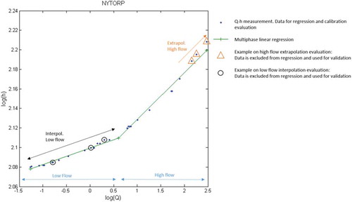
Petersen-Overleir and Reitan (2005) developed a nonlinear regression method with the purpose of achieving an objective segmentation, hence avoiding the risk of errors generated by arbitrary assumptions (Jónsson et al. 2002). To overcome the challenges with multimodality in the likelihood surface when using this nonlinear regression method, the same authors proposed a Bayesian approach (Reitan and Petersen-Overleir 2009), allowing for the determination of an optimal number of segments. The fundamental hypothesis is that segmented rating curves will generate a better fit and fewer errors when there is a clear segmentation in log-log transformed h–Q data.

Yet, regardless of what method is used for building segmented rating curves, each additional segment increases the number of parameters by three for each segment, see Equation (2). Using more parameters in a model based on a limited amount of data increases the risk of over-parameterization and overfitting.

Overfitting occurs when a model starts to fit both the intended observations as well as the noise (Hawkins 2004). In the case of rating curves, the noise is primarily measurement uncertainty. Overfitting can even generate more uncertainty when extrapolating rating curves (Di Baldassarre et al. 2012). Typically, an increased number of parameters leads to reduced model errors for the data used for calibration, but it can also deteriorate the predicting accuracy for similar but independent data, especially if calibration data are scarce and data variance is large (Beven 1993, Jakeman and Hornberger 1993). On the other hand, having too few model parameters can generate a prediction bias by not explaining the reality well enough. Setting the right number of model parameters can be regarded as a trade-off function of bias and variance, where the minimum represents the right number of parameters (Faber and Rajko 2007, Di Baldassarre et al. 2012). The general principle about the number of model parameters is parsimony, which means the least number of predictors should be used to explain the relationship under study (Hawkins 2004). Thus, segmentation of rating curves was evaluated on a large number of gauging stations and included the primary source of data noise, i.e. uncertainty in the direct measurements of stage and discharge. Important and practical variables were also considered, e.g. the sign of segmentation (differences in the slopes of the segments) and the number of direct measurements (sample size).

2 Methods

2.1 Model validation set-up

A conventional procedure to evaluate model performance and test the presence of overfitting is model validation (Faber and Rajko 2007), such as residual validation analysis (Doherty and Hunt 2009).

Unsegmented and segmented rating curves were constructed by using stage and discharge measurements from SMHI’s gauging network. A total of six variations was compared by estimating unsegmented, upper segment (representative of high-flow conditions) and lower segment (representative of low-flow conditions) rating curves with two different regression methods. They were evaluated in calibration, interpolation and extrapolation.

For segmented rating curves, the measurements from each gauging station were divided into an upper segment and a lower one. The separation was done by identifying the intersection, (Equation (2)), from the optimal fit of two linear regressions on the logarithmic scale, performed with a multiphase linear regression (Fig. 1) (Hudson 1966, Ganse 2015). From theory, a difference in slope of the two sections on the logarithmic scale should indicate segmentation in the cross-section of the corresponding gauging station. Since the objective of this study was primarily to evaluate segmentation (and not numerical solving methods), only two numerical solvers were used for regression: the projection variable method and a simpler log method.

To increase the convergence of the regression, the powerful projection variable method was used to solve the separable nonlinear least squares problem of Equation (1) (as in Petersen-Overleir and Reitan 2005). The linear parameters, in this case , can be expressed as a function, , of the nonlinear parameters and (Equation (4)) (Golub and Pereyra 2003). This reduces the number of parameters and increases convergence towards a global minimum if given proper initial guesses and boundaries of the nonlinear parameters (Equation (3)). Parameter boundaries given in the iterative algorithms were > 0, [1, 5] and > 0. Due to an unrealistically high occurrence of parameter converging to = 0, rating curves with = 1 ± 0.001 and = 5 ± 0.001 were removed.

(3)

(4)

The log method is simpler, intuitive and easy to implement. It uses the linear properties of log-log transformed h–Q data, as in Figure 1. The intersection on the y-axis of the linear regression is determined as, or the stage of no flow. An additional linear regression is subsequently used to determine and .

Three types of evaluation were made: calibration, interpolation and extrapolation. From each gauging station, one-third (rounded upwards) of all available measurement data in the segmented rating curve were used for validation. The rest of the data were used to construct the rating curve (Equation (1)). In interpolation, for upper and lower segments, respectively, one-third of the data were randomly extracted and used for validation. For calibration, the same data as in the interpolation were not extracted, but used for error measurements. For extrapolation, the uppermost and lowermost thirds of the data were used for validation. The common external validation method was used, by dividing the available data into a training set and a validation set. The widely used 30%, discretely rounded upwards, were assessed (recommended by Carlsson 2014), ensuring enough data for both training and validation.

2.2 Monte Carlo simulation

A discharge measurement is often interpreted as a rigid data point, when it is a representation of discharge error distribution. Petersen-Overleir and Reitan (2005) suggests that a h–Q data should rather be regarded as a normal distribution, where the variance depends on the measurement error, Stage errors, , are commonly expressed in cm (Equation (5)), while discharge errors, , are generally expressed in percentage (Equation (6)), being the mean and the variance:

(5)

(6)

The stage was simulated with 3 cm uncertainty (the largest stage error mentioned) and the discharge with 1, 5 and 10% uncertainty (e.g. Pappenberger et al. 2007, Di Baldassarre and Montanari 2009). All rating curves were built 100 times with the original data resampled with simulated errors from Equations (5) and (6). By stepwise increasing the measurement uncertainty in Equations (5) and (6), we estimated the uncertainty in rating curves and determined whether segmented rating curves are overfitted or not (Faber and Rajko 2007). In particular, we considered the presence of overfitting, when the extrapolation errors grow faster for the segmented curves than for the unsegmented ones.

2.3 Slope ratio and number of measurements

An important aspect in the construction of rating curves is to explore under which conditions there is an advantage in using segmented rating curves compared to unsegmented. A practical variable for hydrologists is the number of direct measurements needed for the parameterization of a rating curve, and if there is a strong enough indication in the log-log transformation of h–Q data to motivate a segmentation. A sign of segmentation was quantified as a small slope ratio:

(7)

A slope ratio close to 1 indicates no sign of segmentation, and the closer to 0 the slope ratio is, the stronger the sign of segmentation. Simulations were therefore done by extracting gauging stations with a small slope ratio. A reasonably clear indication of segmentation was (arbitrarily) set to a slope ratio <0.2. Linear regressions were also made to evaluate the relation of a sign of segmentation with the rating curve performance.

Another essential variable under evaluation was the number of measurements used for rating curve construction. More measurements would theoretically stabilize the rating curve and reduce the impact of measurement uncertainty. To identify such a relationship, rating curves with equal numbers of measurements were plotted against their corresponding median error and variance. For all experiments in this paper, resampling was done 1000 times with the Monte Carlo method and relative errors larger than 500% were considered outliers and removed.

2.4 Measuring the goodness of fit

Comparisons of regression performance by validation analysis were quantified by residuals analysis, which is based on the difference between simulated values and observed values. The commonly used root mean square error (RMSE) estimate was used, where is the residual error, the modelled discharge, the measured discharge validation data and the number of validation measurements:

(8)

(9)

All rivers and streams have different hydrological variability. Thus, to make results comparable, the absolute flow errors were normalized by dividing with the mean flow of the validation measurements. The procedure allowed an estimation of the mean relative error for each rating curve, which can be viewed as average relative uncertainty in the range of validation data:

(10)

2.5 Uncertainty in stage discharge measurements

The study used active h–Q data from the Swedish gauging network managed by the SMHI (Swedish Meteorological and Hydrological Institute). The stations are distributed throughout the country and the network consists of around 230 gauging stations under varying conditions and discharge magnitudes (Lennermark 2015). At the SMHI, the error in stage measurement should not be greater than ±3 mm according to ISO 1100-2 (1998), but the practical threshold is ±10 mm (Sjödin 2009). McMillan et al. (2012) suggest that uncertainty is typically less than ±10 mm, but local water oscillations and clogging of stilling wells can add another ±20 mm uncertainty (Van der Made 1982, Dottori et al. 2009).

For measuring discharge, mechanical current meters were predominantly used until the middle of the 1990s, and some of these measurements are still being used in today’s rating curves (Goltsis Nilsson 2014, SMHI 2014). A comprehensive literature review on mechanical current meters indicated a discharge measurement uncertainty of 4–17% (Pelletier 1988, McMillan et al. 2012). The mechanical current meters have mostly been replaced with various acoustic Doppler current profilers (ADCP) by SMHI during the last 20 years (SMHI 2014). Uncertainties in boat-held ADCP are often calculated from several measured transects and the difference from each transect is the relative uncertainty. Studies have shown errors of, on average, 3–5% or 5–7% when comparing several transects (Mueller 2003). A third, but less practiced, method in Sweden is salt injections (SMHI 2014). Studies have shown uncertainties of 2.3–7.1% in salt dilution discharge measurement in small turbulent streams (Hamilton and Moore 2012).

3 Results

3.1 Calibration, interpolation and extrapolation

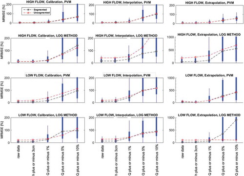
Figure 2 shows the errors of rating curves and highlights that the uncertainty in direct measurements of discharge has a major impact. Also, errors are generally larger for low flows than high flows, especially in extrapolation (Fig. 2). Generally, the projection variable method leads to rating curves with fewer errors than the log method, with the exception of unsegmented rating curves in low flows (Fig. 2, bottom right). In some cases, segmented rating curves perform slightly better than unsegmented ones, but differences are usually very small. However, this seems not to hold true for low-flow extrapolation with the log method. Lastly, no obvious signs of over-parameterization can be observed in the results.

Figure 2. Boxplots of the median distributions of calibration, interpolation and extrapolation MRMSE for high and low flows, when segmented and unsegmented rating curves were constructed with varying measurement uncertainty. PVM: projection variable method (Equation (5)); LOG: linear regression on log-log transformed h–Q data; h ± 3cm: stage measurement uncertainty of 3 cm; Q ± 1%, Q ± 5% and Q ± 10%: discharge measurement uncertainty of 1, 5 and 10%, respectively; raw data: no resampling without uncertainty.

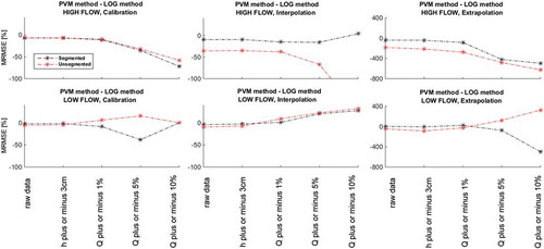
Comparing the two different regression models, it is possible to observe that the projection variable method generally generates less error for high flows compared to the log method, shown in Figure 3. The log method performs with fewer errors in low flows, with the exception of segmented rating curves in extrapolation.

Figure 3. Difference in error (MRMSE) between the projection variable method (PVM) and the log method for calibration, interpolation and extrapolation for high and low flows, for both unsegmented and segmented rating curves. Negative values on the y-axis indicate that the PVM generates less error than the log method.

3.2 Slope ratio

A small slope ratio (<0.2, Equation (7)) indicates a clear visual segmentation and therefore motivates the use of segmented rating curves. When the analysis is applied on rating curves with slope ratios <0.2, it is possible to observe that the impact of segmentation is small for high flows (Fig. 4). For very low measurement uncertainties there is a positive impact of segmentation on low flows, but when accounting for discharge measurement uncertainties larger than 1%, unsegmented rating curves perform better in both interpolation and extrapolation. It is noteworthy that rating curves with slope ratio <0.2 generate more errors for low flows compared to the general results shown in Figure 3 (Fig. 4).

Figure 4. Boxplots of the median distributions of calibration, interpolation and extrapolation MRMSE for high and low flows, when segmented and unsegmented rating curves were constructed with varying measurement uncertainty and slope ratio < 0.2.

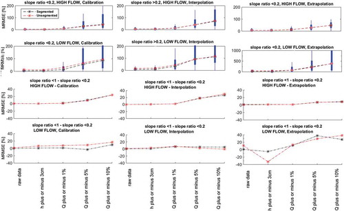
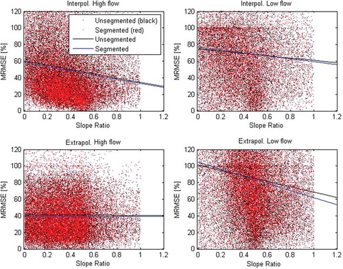
Figure 4 shows the difference in MRMSE between rating curves with slope ratio <0.2 and the total set of rating curves (slope ratio <1 to slope ratio <0.2); negative values on the y-axis indicate that the whole set of rating curves generates less error than rating curves with a slope ratio <0.2. A small slope ratio (<0.2) generally generates more errors for all types of rating curves. Regression between slope ratio and error confirms that a small slope ratio generates a larger error (Fig. 5). For low flows, in both interpolation and extrapolation, the segmented rating curve performs with fewer errors, with a slope ratio of less than 0.3–0.4 (Fig. 5). It is also worth observing that the density of rating curves with a smaller slope ratio compares to that with a larger slope ratio, indicating that the majority of rating curves have a degree of segmentation in the log-log space.

Figure 5. Distribution and linear regression of MRMSE in interpolation and extrapolation for high (left) and low (right) flows, with the slope ratio (Equation (7)) as the variable. A small slope indicates segmentation; only slope ratios between 0 and 1 were included. Segmented and unsegmented rating curves were constructed with the projection variable method and a discharge measurement uncertainty of 5% (Equation (5)).

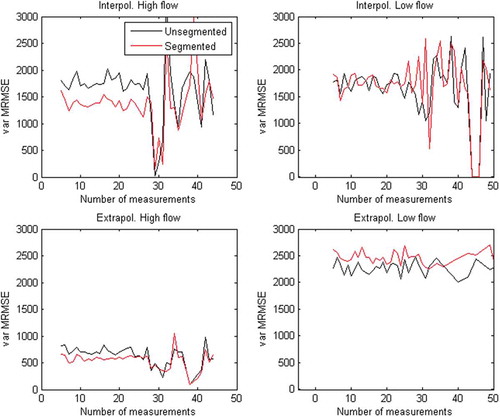
The number of measurements ranging between 1 and 30 does not have a noteworthy effect on the distribution in either of the rating curve segmentation methods (Fig. 6). More than 25 measurements are rare in the dataset, hence the high variance in Figure 6. Although there was no difference in absolute errors, segmentation clearly generated less variance for high flows when the number of measurements was less than 25 (Fig. 7). Besides the comparison between the segmentation methods, neither the absolute error nor variance was reduced by increasing the number of measurements.

Figure 6. Median MRMSE in interpolation and extrapolation for high (left) and low (right) flows, with the number of measurements as the variable. Segmented and unsegmented rating curves were constructed with the projection variable method and a discharge measurement uncertainty of 5% (Equation (5)).

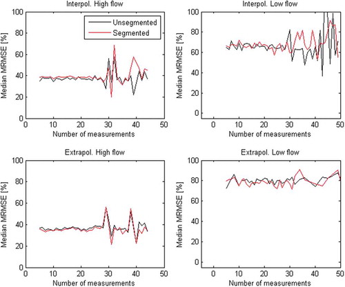
Figure 7. Variance of MRMSE in interpolation and extrapolation for high (left) and low (right) flows, with the number of measurements as the variable. Segmented and unsegmented rating curves were constructed with the projection variable method and a discharge measurement uncertainty of 5% (Equation (5)).

4 Discussion and conclusions

The suggested improvement of the rating curve method, by segmenting the power law rating curve (Equation (2)) (Petersen-Overleir and Reitan 2005, Reitan and Petersen-Overleir 2009), was evaluated on over 230 rating curves for Sweden. Large differences of errors in the rating curves emerged when measurement uncertainties were accounted for. Figure 2 shows errors for unsegmented rating curves. The median error in calibration of high flow was estimated to be around 4%. However, when an average measurement uncertainty of ±5% was included, the median error from the rating curves was estimated to be close to 60% (Fig. 2). If the same measurement uncertainty was considered when extrapolating, the median error was about 36%. The latter is similar to previous studies indicating uncertainty in high-flow data as high as 30–40% (Di Baldassarre and Montanari 2009). Percentage errors in extrapolation for high flows can be smaller than percentage errors in interpolation. The reason for this is that extrapolation was measured at a higher discharge only, and the larger the discharge the smaller the relative errors become, especially if compared to errors in low-flow conditions. In fact, this is not the case for low-flow conditions, in which the median error in calibration was 41% (Fig. 2), while for a ± 5% measurement uncertainty the median error was 95% in interpolation and 250% when extrapolating to low-flow conditions (Fig. 2).

The results show that the projection variable method generally constructs rating curves with the least amount of errors compared to the simpler log method, for both segmented and unsegmented rating curves (Fig. 2). These results were strongest for high flows, but the projection variable method performs equally with the log method for low flows. The exception was that the log method generates considerably smaller errors in extrapolation for low-flow unsegmented rating curves. This can be attributed to the fact that a regression with the log method reduces effects of heteroscedasticity, whereas regression on non-transformed h–Q data (in this case the projection variable method) gives more weight to high discharge values.

When it comes to the performance of segmentation with the projection variable method, only minor differences could be observed in calibration, interpolation or extrapolation (Fig. 2). For the log method, segmented rating curves showed that they often performed with fewer errors compared to unsegmented rating curves.

When simulating cross-sections at gauging stations that have a clear sign of segmentation (slope ratio <0.2), those rating curves generated more errors than curves with less sign of segmentation (larger slope ratios) (Fig. 4). Regressions showed clear trends between slope ratio and errors (Fig. 5). Yet the hypothesis that a stronger sign of segmentation (small slope ratio) should motivate segmented rating curves was confirmed only on low flows (Fig. 5), where segmentation was preferred when the slope ratio was less than 0.3–0.4. This could be an indicator that segmented rating curves could suffer from over-parameterization. Surprisingly, the number of measurements did not have a large impact on either the magnitude of the errors or the variance (Figs 6 and 7). It can be argued that the benefits of using the two segmentation methods are too small to justify the sophisticated work of building segmented rating curves. It should also be said, however, that while the benefits of using segmentation are small, the approach rarely worsen the errors. In other words, segmentation of rating curves had little or no positive impact on rating curve performance in calibration, interpolation or extrapolation, for high or low flows. Instead, segmented rating curves showed only slight signs of over-parameterization, meaning that segmentation of rating curves did not generate more errors. Rating curves with a clear segmentation (small slope ratio) generally generated more errors and, when this occurred, segmentation had a positive impact on low-flow conditions for slope ratios of less than 0.3–0.4.

Lastly, this study showed that accounting for even small measurement uncertainties led to much larger errors in discharge data from rating curves. As expected, streamflow inaccuracy had the largest impact on errors generated from rating curves, while stage measurement uncertainty had an almost negligible impact. Assuming a discharge uncertainty of ±5%, errors in high-flow conditions were about 36% in extrapolation. For low flows, extrapolation errors can be as high as 250%.

Disclosure statement

No potential conflict of interest was reported by the authors.

References

- Beven, K., 1993. Prophecy, reality and uncertainty in distributed hydrological modeling. Advances in Water Resources, 16, 41–51. doi:10.1016/0309-1708(93)90028-E
- Carlsson, 2014. Personal communication, Uppsala University, Uppsala, 20 October
- Di Baldassarre, G. and Claps, P., 2011. A hydraulic study on the applicability of flood rating curves. Hydrology Research, 42 (1), 10–19. doi:10.2166/nh.2010.098
- Di Baldassarre, G., Laio, F., and Montanari, A., 2012. Effect of observation errors on the uncertainty of design floods. Physics and Chemistry of the Earth, 42–44, 85–90. doi:10.1016/j.pce.2011.05.001
- Di Baldassarre, G. and Montanari, A., 2009. Uncertainty in river discharge observations: a quantitative analysis. Hydrology and Earth System Sciences, 13, 913–921. doi:10.5194/hess-13-913-2009
- Doherty, J. and Hunt, R.J., 2009. Two statistics for evaluating parameter identifiability and error reduction. Journal of Hydrology, 366, 119–127. doi:10.1016/j.jhydrol.2008.12.018
- Domeneghetti, A., Castellarin, A., and Brath, A., 2012. Assessing rating-curve uncertainty and its effects on hydraulic model calibration. Hydrology and Earth System Sciences, 16 (4), 1191–1202. doi:10.5194/hess-16-1191-2012
- Dottori, F., Martina, M.L.V., and Todini, E., 2009. A dynamic rating curve approach to indirect discharge measurement. Hydrology and Earth System Sciences, 13, 847–863. doi:10.5194/hess-13-847-2009
- Faber, N.M. and Rajko, R., 2007. How to avoid over-fitting in multivariate calibration - the conventional validation approach and an alternative. Analytica Chimica Acta, 595, 98–106. doi:10.1016/j.aca.2007.05.030
- Fenton, J.D., 2001. Rating curves: part 2 – representation and approximation. In: 6th Conference on Hydraulics in Civil Engineering: The State of Hydraulics; Proceedings, Vol. 1, 28–30 November. Barton, ACT: Institution of Engineers, Australia, Tasmania, Hobart, 319–328.
- Ganse, A.A., 2015. Multi-phase linear regr. Available from: http://staff.washington.edu/aganse/mpregression/mpregression.html [Accessed 4 December 2015].
- Goltsis Nilsson, M., 2014. SMHI, Personal communication, 17 March.
- Golub, G. and Pereyra, V., 2003. Separable nonlinear least squares: the variable projection method and its applications. Inverse Problems, 19, R1–R26. doi:10.1088/0266-5611/19/2/201
- Hamilton, A.S. and Moore, R.D., 2012. Quantifying uncertainty in streamflow records. Canadian Water Resources Journal, 37, 3–21. doi:10.4296/cwrj3701865
- Haque, M., Rahman, A., and Haddad, K., 2014. Rating curve uncertainty in flood frequency analysis: a quantitative assessment. Journal of Hydrology and Environmental Research, 2 (1), 50–58.
- Hawkins, D.M., 2004. The problem of overfitting. Journal of Chemical Information Modeling, 44, 1–12.
- Herschy, R.W., ed., 1999. Hydrometry: principles and practices. 2nd ed. New York: John Wiley.
- Hudson, D., 1966. Fitting segmented curves whose join points have to be estimated. Journal of the American Statistical Association, 61, 1097. doi:10.1080/01621459.1966.10482198
- ISO 1100-2, 1998. Measurement of liquid flow in open channels - part 2: determination of the stage–discharge relation. Geneva: International Standards Organization.
- Jakeman, A. and Hornberger, G., 1993. How much complexity is warranted in a rainfall–runoff model. Water Resources Research, 29, 2637–2649. doi:10.1029/93WR00877
- Jónsson, P., et al., 2002. Methodological and personal uncertainties in the establishment of rating curves, NHP Report No. 47. XXII Nordic Hydrological Conference, (1).
- Kuczera, G., 1996. Correlated rating curve error in flood frequency inference. Water Resources Research, 32, 2119–2127. doi:10.1029/96WR00804
- Lambie, J.C., 1978. Measurement of flow–velocity–area methods. 1st ed. Chichester: Wiley.
- Lang, M., et al., 2010. Extrapolation of rating curves by hydraulic modelling, with application to flood frequency analysis. Hydrological Sciences Journal, 55 (6), 883–898. doi:10.1080/02626667.2010.504186
- Lennermark, M., 2015. SMHI, Personal communication, 12 July.
- McMillan, H., Krueger, T., and Freer, J., 2012. Benchmarking observational uncertainties for hydrology: rainfall, river discharge and water quality. Hydrological Processes, 26, 4078–4111. doi:10.1002/hyp.v26.26
- Mueller, D.S., 2003. Field evaluation of boat-mounted acoustic doppler instruments used to measure streamflow. Proceedings of the IEEE Working Conference on Current Measurement, 1, 30–34.
- Pappenberger, F., et al., 2006. Influence of uncertain boundary conditions and model structure on flood inundation predictions. Advances in Water Resources, 29, 1430–1449. doi:10.1016/j.advwatres.2005.11.012
- Pappenberger, F., et al., 2007. Grasping the unavoidable subjectivity in calibration of flood inundation models: a vulnerability weighted approach. Journal of Hydrology, 333, 275–287. doi:10.1016/j.jhydrol.2006.08.017
- Pelletier, P., 1988. Uncertainties in the single determination of river discharge - a literature review. Canadian Journal of Civil Engineering, 15, 834–850. doi:10.1139/l88-109
- Pena-Arancibia, J.L., et al., 2015. Streamflow rating uncertainty: characterisation and impacts on model calibration and performance. Environmental Modelling and Software, 63, 32–44. doi:10.1016/j.envsoft.2014.09.011
- Petersen-Overleir, A., 2009. Avbördningskurvan ur ett hydrauliskt perspektiv. Available from: https://www.smhi.se/polopoly_fs/1.8909!/08_Asgeir_Petersen-Overleir.pdf [Accessed 6 August 2017].
- Petersen-Overleir, A. and Reitan, T., 2005. Objective segmentation in compound rating curves. Journal of Hydrology, 311 (1–4), 188–201. doi:10.1016/j.jhydrol.2005.01.016
- Reitan, T. and Petersen-Overleir, A., 2009. Bayesian methods for estimating multi-segment discharge rating curves. Stochastic and Environmental Research Risk Assessment, 23 (5), 627–642. doi:10.1007/s00477-008-0248-0
- Sjödin, N., 2009. Dagens ISO-standard för fältmätning av vattenstånd och vattenföring. Sweden, Norrköping, SMHI. Available from: https://www.smhi.se/polopoly_fs/1.8903!/02_Nils_Sj%C3%B6din.pdf [Accessed 10 October 2015]..
- SMHI, 2014. SMHIs vattenföringsmätningar. SMHI. Available from: http://www.smhi.se/kunskapsbanken/hydrologi/smhis-vattenforingsmatningar-1.80833 [ Accessed 4 October 2015].
- Strömqvist, J., et al., 2012. Water and nutrient predictions in ungauged basins: set-up and evaluation of a model at the national scale. Hydrological Sciences Journal, 57 (2), 229–247. doi:10.1080/02626667.2011.637497
- Van der Made, J., 1982. Determination of the accuracy of water level observations. In: Advances in hydrometry (Proceedings of the Exeter Symposium, July 1982). Wallingford, UK: IAHS, 173–184. IAHS Publ. 134. Available from: http://iahs.info/uploads/dms/134019.pdf [ Accessed 10 August 2017].
- Westerberg, I.K., et al., 2016. Uncertainty in hydrological signatures for gauged and ungauged catchments. Water Resources Research, 52, 1847–1865. doi:10.1002/2015WR017635
- WMO (World Meteorological Organization), 2008. Guide to hydrological practices. 6th ed. Geneva, Switzerland: WMO.