Prediction of flow rate of karstic springs using support vector machines

ABSTRACT

Complex void space structure and flow patterns in karstic aquifers render behaviour prediction of karstic springs difficult. Four support vector regression-based models are proposed to predict flow rates from two adjacent karstic springs in Greece (Mai Vryssi and Pera Vryssi). Having no accurate estimates of the groundwater flow pattern, we used four kernels: linear, polynomial, Gaussian radial basis function and exponential radial basis function (ERBF). The data used for training and testing included daily and mean monthly precipitation, and spring flow rates. The support vector machine (SVM) performance depends on hyper-parameters, which were optimized using a grid search approach. Model performance was evaluated using root mean square error and correlation coefficient. Polynomial kernel performed better for Mai Vryssi and the ERBF for Pera Vryssi. All models except one performed better for Pera Vryssi. Our models performed better than generalized regression neural network, radial basis function neural network and ARIMA models.

KEYWORDS:

• groundwater flow
• karst
• support vector machines
• spring flow rate
• precipitation
• artificial neural networks

Editor A. Castellarin; Associate editor A. Jain

1 Introduction

Karst is a special type of landscape, resulting from dissolution of soluble rocks including limestone, dolomite, marble and gypsum. Karstic landforms are sometimes absent at the surface, but groundwater can be karstic. Rainfall, coming in contact with carbon dioxide present in the atmosphere and soil, becomes acidic. When this acidic rainwater percolates into the rocks through fractures, it dissolves the soluble material and forms networks of passages for itself. This process of dissolution of rocks keeps happening over time, finally leading to a gradual increase in the size and network of passages. These passages ultimately become caves, springs, sinkholes and tunnels. Water enters the karst system through recharge areas, flows through void spaces of different size and leaves from discharge areas (springs). The discharge and transit time of these aquifers depend on the void space size and geometry, soil moisture, recharge event intensity and duration, and the type of rocks present. Many of these factors are generally not known; for this reason, it is difficult to predict the behaviour of karstic aquifers and flow of karstic springs.

A large part of the world’s population (roughly 20–25%) depends on groundwater obtained from karstic aquifers, and large ice-free continental areas (e.g. 35% of Europe) are underlain by karst, formed on carbonate rocks (Ford and Williams 2007). Due to its practical importance, scientific literature on karstic aquifers and springs is very extensive. Halihan et al. (1998) studied the physical response of a karst drainage basin to flood pulses. Based on the application of Bernoulli’s equation, the study indicated localized control during storm events. Jeannin (2001) studied the hydrodynamic properties of karst conduits by considering them as a network of pipes with impervious irregular walls. Peterson and Wicks (2006) used a storm water management model (SWMM) for assessing the importance of conduit geometry and physical parameters in karst systems. They found that changes in length or width of the conduits produced significant variation in flow responses, whereas slope and infiltration rates had minimal effect. Further, they found that a small change in Manning’s roughness coefficient highly altered the simulated output. Sepulveda (2009) compared hydraulically and statistically based methods to predict spring flows in a karst aquifers. The Hantush-Jacob and Darcy-Weisbach equations were used for hydraulically based methods, while multiple linear equations and artificial neural networks (ANNs) were used for statistically based methods. The ANNs were found to predict karstic spring flows accurately, at least when there were abundant field data (e.g. Hu et al. 2008). Paleologos et al. (2013) used ANNs to predict the flow of two karstic springs based on rather restricted field data. The predictions of the neural network captured the behaviour of both springs and the under/overestimation remained below 3% with some exceptions. They also investigated the problem by including artificial data, but no improvement was found. The inclusion of past discharge data in the input improved the predictions.

In this paper, we use support vector machines (SVM) to predict the discharge of karstic springs. The concept of SVM was introduced by Vapnik (1995). It is based on the structural risk minimization (SRM) principle, which is shown to be better than the traditional empirical risk minimization (ERM) principle, as it tries to find a decision rule that provides good generalization by selecting some subset of training data, called support vectors. Input space is nonlinearly mapped to a higher-dimensional feature space using kernels to account for nonlinearity. Support vector machines, which are further discussed in Section 4, have been already used in water resources management. Sivapragasam et al. (2001) used a hybrid model by coupling singular spectrum analysis (SSA) with SVM for rainfall and runoff forecasting. Raghavendra and Deka (2014) presented many SVM-based models used in the field of hydrology. The SVM have also been widely used during the last decade for rainfall–runoff modelling (e.g. Dibike et al. 2001, Bray and Han 2004), streamflow forecasting (e.g. Lin et al. 2006, Shabri and Suhartono 2012, Zakaria and Shabri 2012), groundwater hydrology (e.g. Behzad et al. 2010, Liu et al. 2009), groundwater contamination (e.g. Dixon 2009), estimation of scouring (Goyal and Ojha 2011), estimation of suspended sediments in rivers (Çimen 2008), and conjunctive use of surface and groundwater (Safavi and Esmikhani 2013). Liu et al. (2011) established a SVM-based multiple-factor water quality assessment model, which solved the complex nonlinear relationship between assessment factor and water quality grade with high prediction accuracy. Not much work has been done on the application of SVM for flow prediction in karstic aquifers to the knowledge of the authors.

2 Study area

Karsts are very common in Europe, where around one-third of the surface area contains karstic springs. Greece is home to many karstic waters, e.g. South Parnassos and Ghiona aquifers, Parnitha-Pateras and Hymittos aquifers, Almyros springs, Aggitis springs (Novel et al. 2007, Tsakiris et al. 2009, Kallioras and Marinos 2015). Carbonate rocks cover more than 35% of the country (EASAC 2010).

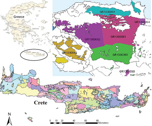
The current study is based on two perennial karstic springs (Mai Vryssi and Pera Vryssi) in Gergeri village of the municipality of Rouva in southern central Crete, Greece (Fig. 1). These two springs are separated by a distance of 800 m and their elevation is approx. 500 m a.s.l., whereas the area that feeds them is at an average elevation of 950 m a.s.l. There are more springs, some of them on rough terrain (Darivianakis 2011, Darivianakis et al. 2015). The springs are fed by the karstic system of Notios (South) Psiloreitis (GR1300065), which has an average elevation of 900 m and is shown in Figure 1 (Kritsotakis and Pavlidou 2013).

Figure 1. Study area (Rouvas area, Crete, Greece). Based on Kritsotakis and Pavlidou (2013).

Monthly rainfall data for the years 2006–2010 appear in Table 1. The most prominent feature is that June, July and August were practically rainless. It is also worth mentioning that three successive years, 2006, 2007 and 2008, had similar annual rainfall (800–841.8 mm/year). A wet year followed and then a dry one. The average annual precipitation for the 35-year period (1965–1999) is 838.9 mm/year, so there is no obvious annual rainfall reduction trend.

Table 1. Monthly precipitation data for the period 2006–2010.

	Jan	Feb	Mar	Apr	May	Jun	Jul	Aug	Sep	Oct	Nov	Dec	Year
2006	78.1	110.3	113.0	48.5	3.5	0.0	0.0	0.0	15.5	110.7	342.7	19.5	841.8
2007	59.5	161.0	75.0	7.2	53.1	4.0	0.0	0.0	0.0	179.5	82.0	178.7	800.0
2008	124.5	146.5	28.5	67.0	4.1	0.0	0.0	0.0	25.0	7.5	159.5	237.5	800.1
2009	295.3	178.0	52.5	57.6	30.2	0.0	0.0	0.0	63.5	54.5	99.0	225.6	1056.2
2010	220.6	75.3	4.8	7.5	0.0	2.4	0.3	0.0	0.0	84.6	60.4	110.1	566.0

3 Data used in SVM models

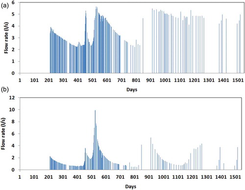
Data on daily rainfall and spring flow rates were obtained from Darivianakis et al. (2015). In that paper, the authors used ANN techniques to predict the flow rate at these two springs. A complete set of daily rainfall data is available from 20 September 2006 to 16 December 2010. This set, which was obtained from a rain gauge installed near the Pera Vryssi spring, is concisely presented in Figure 2. Spring flow rate measurements are available for 268 days between 16 April 2007 and 16 December 2010, and their collection followed a rather irregular pattern. Measured flow rates at Mai Vryssi and Pera Vryssi springs are shown in Figure 3(a) and (b), respectively. High peaks and low baseflow are observed for Pera Vryssi, whereas for Mai Vryssi low peaks are observed with a significant amount of baseflow. This different behaviour has been also observed by local residents (Darivianakis et al. 2015). The peaks in flow rate occur a few days after high rainfall events. Our calculations have shown that the lag is different for the two springs. The perennial flow of both springs indicates that the karstic aquifers is coupled with another groundwater system, allowing low groundwater velocities and serving as a “deep compartment” (the term is borrowed from pharmacokinetics).

Figure 2. Bar chart showing daily rainfall (mm) from 20 September 2006 to 16 December 2010.

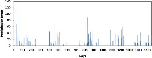
Figure 3. Bar charts showing measured flow rates (L/s) at (a) Mai Vryssi spring and (b) Pera Vryssi spring.

4 Outline of support vector regression (SVR)

The support vector machine (SVM) is a method of supervised learning used for classification and regression analysis. It was developed by Vapnik and his team at AT&T’s Bell Labs, based on statistical learning theory. Support vector regression (SVR) is briefly outlined below.

Consider a simple linear regression problem trained on the dataset (X,Y), where is the input dataset and is the target set. The objective is to find a function f(x) which links the input data points to target data points in the training dataset:

(1)

where w is the weight vector and b is the bias term. This function can later be used to find y_i based on some new inputs (x_i). The term w·x is the dot product between w and x.

In SVR, a loss function, , is used, which describes the deviation of function f(x) outcomes from the actual target values (y_i). Different types of loss functions are presented in the literature. This allows some deviation between the target values y_i and the function values . The Vapnik ε-insensitive loss function is used here, which is defined as:

(2)

Only the points lying outside the ε-insensitive zone contribute to the “cost” and the deviations are penalized in a linear fashion. The associated convex quadratic programming problem can be written as:

(3)

(4)

where and are slack variables, which represent the deviation of training data points outside the ε-insensitive zone. The slack variables are zero for points inside the ε-insensitive zone and increase progressively for points outside the zone. The term C is a regularization constant, which assigns a penalty when a training error occurs. It turns out that the optimization problem can easily be solved in the dual form.

The Lagrange function is constructed from the primal objective function and the corresponding constraints, by introducing a dual set of variables, and . It can be shown that this function has a saddle point with respect to the primal and dual variables of the optimal solution. The dual formation of the optimization problem is:

(5)

Subject to:

(6)

After determining the Lagrange multipliers, and , the Karush-Kuhn-Tucker (KKT) method is used to find the parameters and . Prediction in a linear regression function can be expressed as:

(7)

In order to use SVR in nonlinear cases, the decision space variable (X) can be mapped to a higher-dimensional space, using function . Applying this transformation, the dual problem becomes:

(8)

(9)

where is called the kernel function. Any function that satisfies Mercer’s theorem can be used as kernel (Vapnik 1999).

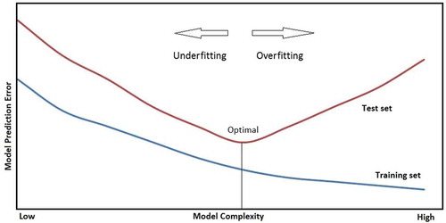
The hyper-parameters such as the SVR constant ε, regularization constant C and σ (for radial basis function kernels) influence the success of the SVR. Parameter C allows a trade-off between training error and model complexity. If a model is not sufficiently complex, then it may fail to capture the underlying trend of the data and hence cause underfitting. On the other hand, if the model is too complex, it may capture noise of the data, and hence can suffer from overfitting (Fig. 4). A good trade-off between the model complexity and prediction error is a must. A small value of C will increase the number of training errors, hence it tends to underfit the training data, whereas a large value of C will lead to behaviour similar to that of a hard-margin SVM, hence it will tend to overfit the training data (Joachims 2002). The parameter ε controls the width of the ε-insensitive zone and influences the number of support vectors. Hence, its value affects both complexity and generalization capability of the approximation function. Low values of ε lead to a larger number of support vectors and increase the complexity, while high values of ε lead to a smaller number of support vectors and result in more flat estimates of the regression function. The performance of SVR is sensitive to these parameters, so it is important to find appropriate values for C and ε (Kim 2003). Determining the appropriate value of these parameters is often a heuristic trial-and-error process (Raghavendra and Deka 2014).

Figure 4. Model complexity vs performance.

5 Model construction

In this paper, the SVR approach is used to predict the flow rate at the karstic springs of Mai Vryssi and Pera Vryssi, as described in Section 2. Following Darivianakis et al. (2015), we aim mainly to obtain practically useful predictions, that is, to estimate spring flow rates at least a few days in advance. This target is plausible, since the peaks in flow rate are observed to occur a few days after rainfall (Darivianakis 2011).

The prediction ability of a forecasting model depends on the selection of predictor variables and the features and parameter values used in the SVR approach. To compare the performance of different SVR approaches both to each other and to the performance of the ANN, four different models were constructed using different sets of predictor variables:

Model I: Prediction of spring flow rates based on past daily and monthly mean rainfall data.

Model II: Prediction of spring flow rates based on past monthly mean rainfall data only.

Model III: Prediction of spring flow rates for seasonal data only.

Model IV: Prediction of the flow rate at one spring based on flow rate at the other spring on the same day and on past monthly mean rainfall data.

Model I was expected to have the best performance and it was used mainly to check the efficiency of SVM in providing useful results. Model II was aimed at exploring the possibility of providing a rough medium-term forecast. We used Model III in order to investigate whether spring flow rate predictions could be based on seasonal data only. Finally, Model IV was aimed at investigating the possibility of restricting field measurements (and the respective cost) to one spring only.

5.1 Model I

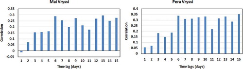
The predictors used for this model include daily and monthly mean rainfall. We examined different input data and selected those offering the best correlation between rainfall and spring flow rates. This correlation for time lags of 1–15 days is shown in Figure 5, for both springs. For Mai Vryssi, time lags of 6, 7, 9, 12, 13 and 15 days and mean monthly rainfall data with lags of 1, 2 and 3 months were chosen. For Pera Vryssi, time lags of 6, 9, 10, 12, 13 and 15 days and mean monthly rainfall data with lags of 1, 2, 3 and 6 months were chosen, since a good correlation between flow rate and monthly mean rainfall with 6-month lag was observed for that spring. It should be mentioned that similar (although not exactly the same) correlation results have been reported by Darivianakis et al. (2015).

Figure 5. Correlation between flow rate at two springs and different time lags of rainfall.

To train the model, we used data for 1 year (16 April 2007–15 April 2008), which contain 171 days of flow rate measurements. The rest of the data, including measurements for 91 days, was used for testing the model.

5.2 Model II

The predictors used for this model include mean monthly rainfall only; i.e. the possibility for a rough mid-term forecast is checked. Predictors for Mai Vryssi included mean monthly rainfall with time lags of 1, 2 and 3 months, whereas for Pera Vryssi time lags of 1, 2, 3 and 6 months were used. The model was trained and tested for the same periods as Model I.

5.3 Model III

To check the seasonal forecast ability of the SVR, Model III is developed using seasonal data only. The spring season (March–May) was used in this study and the data for spring 2007 (including 31 flow rate measurements) was used for training, while seasonal data of the remaining years (including 48 measurements) was used for testing.

5.4 Model IV

As both springs are fed by the same catchment, their flow rates could be correlated, despite their different behaviour, as mentioned in Section 3. In this model, the flow rate at one spring is used as a predictor for the other, along with the mean monthly rainfall. For Mai Vryssi, the flow rate at Pera Vryssi of the same day was used, along with mean monthly rainfall with 1-, 2- and 3-month lags, as predictors. Similarly, the same day flow rate at Mai Vryssi and 1-, 2-, 3- and 6-month lags of mean monthly rainfall were used as predictors for Pera Vryssi. Training and testing periods remained the same as those for Model I and Model II.

In all four models, SVR uses kernel functions, to take into account the nonlinearity present in the datasets. The four different types of kernel functions used in this study are shown in Table 2. Linear and radial basis function (RBF) kernels are widely used in SVM studies (e.g. Han et al. 2007, Shahbazi and Pilpayeh 2012). Here we used polynomial and Gaussian radial basis function (GRBF) kernels, too.

Table 2. Different kernel functions used and their respective formulas. RBF: radial basis function.

Kernel	Formula
Linear
Polynomial (homogeneous)
Polynomial (non-homogeneous)
Gaussian RBF
Exponential RBF

A gridded search method was used to find the optimum values of SVM parameters. First, the search was done on a coarse grid and, after finding an optimal range, a fine grid search was done. The value of epsilon (ε) was varied between 0.05 and 2. The ε value for best results was found to be different for the two springs and for different cases. After finalizing the optimum value of ε, different combinations of C and σ (in the case of RBFs) were tried based on a gridded search approach. The value of C was varied between 0 and 1000.

To evaluate the performance of the forecasting models, two statistics, root mean square error (E_RMS) and correlation coefficient (CC), were used. These measures are defined as follows:

(10)

(11)

where N is the number of observations (days in our case), Y_o and Y_c are the observed and predicted values, respectively, and is the mean of the observed values.

For the implementation of the method, we used SVM MATLAB code, given by Araghinejad (2014).

6 Results and discussion

The optimization problem of SVR is solved using the KKT method, as described in Section 4. The results for all the cases are presented in Table 3. For some cases, the results obtained were very poor, so those cases are left blank in the table. The best results were obtained using different kernels and different sets of hyper-parameters for each spring. This seems quite reasonable since the behaviour of the two springs is quite different.

Table 3. Root mean square error (E_RMS) and correlation coefficient (R) statistics for the testing period. GRBF: Gaussian RBF, ERBF: exponential RBF. Values in bold indicate best values.

	ERMS (L/s)		R
Kernel used	Mai Vryssi	Pera Vryssi	Mai Vryssi	Pera Vryssi
Model I
Linear	0.800	0.663	0.526	0.808
GRBF	0.911	0.746	0.617	0.713
ERBF	0.886	0.636	0.589	0.799
Polynomial NH (degree 1)	0.767	0.660	0.526	0.787
Polynomial NH (degree 2)	1.241	–	–	–
Polynomial H (degree 2)	1.320	–	–	–
Model II
Linear	0.841	0.645	0.507	0.794
GRBF	0.894	0.755	0.512	0.697
ERBF	0.889	0.701	0.499	0.767
Polynomial NH (degree 1)	0.829	0.636	0.514	0.799
Model III
Linear	0.618	–	0.476	–
GRBF	1.075	–	0.000	–
ERBF	0.621	–	0.465	–
Polynomial NH (degree 1)	0.418	–	0.398	–
Model IV
Linear	0.829	1.000	0.528	0.772
GRBF	0.898	0.717	0.533	0.762
ERBF	0.887	0.625	0.566	0.812
Polynomial NH (Degree 1)	0.829	1.110	0.528	0.802

For Model I, the best results for Mai Vryssi (E_RMS = 0.767 L/s) were obtained using the degree-1 polynomial kernel with values of ε = 2 and C = 350 (Figs 6(a) and 7(a)). As can be seen in Figure 6(a), the model is able to predict the peak flow (on day 52) but is not able to predict the low flow regions. For Pera Vryssi, the best results (E_RMS = 0.636 L/s) were obtained using the exponential RBF (ERBF) kernel with values of ε = 0.25, C = 300 and σ = 10 (Figs 6(b) and 7(b)). Predicted flow rate, in this case, shows a better agreement with the observed flow rate. Most of the peaks and low-flow regions are well predicted by the model, whereas it fails to predict a major peak (on day 52). The SVR performed better for Mai Vryssi with high values of ε and for Pera Vryssi with low values of ε. Correlation coefficients for Pera Vryssi are found to be better than for Mai Vryssi in every case.

Figure 6. Plots showing observed and estimated flow rates at Mai Vryssi (a, c, e) and Pera Vryssi (b, d, f) for (a, b) Model I, (c, d) Model II and (e, f) Model IV.

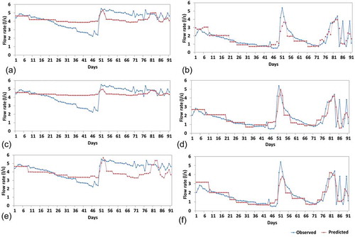
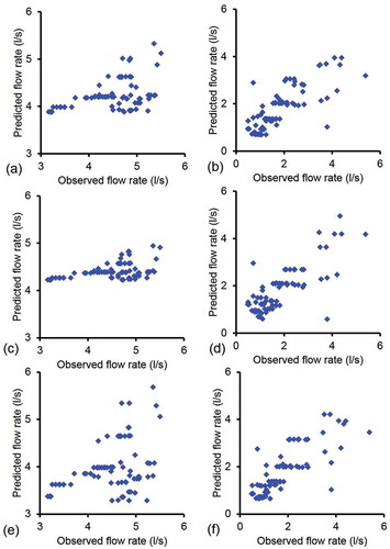
Figure 7. Scatter plots between observed and predicted flow rates at Mai Vryssi (a, c, e) and Pera Vryssi (b, d, f) for (a, b) Model I, (c, d) Model II and (e, f) Model IV.

For Model II the best results were also obtained for Mai Vryssi (E_RMS = 0.829 L/s) using the polynomial kernel of degree 1, with the values of ε = 2 and C = 500 (Figs 6(c) and 7(c)). Figure 6(c) shows that the model predicted the average flow rate, but not the peaks and low flow. For Pera Vryssi the best results (E_RMS = 0.636 L/s) were obtained using the polynomial kernel of degree 1 with the values of ε = 0.05 and C = 300 (Figs 6(d) and 7(d)). Figure 6(d) shows that Model II is able to predict the major peak (on day 52) which was not predicted by Model I. The peak flow is predicted one day later than the actual occurrence of the peak flow. Regarding Mai Vryssi, the performance of SVR for this model was found to be worse (high E_RMS) compared to Model I, as expected. Rather surprisingly, the E_RMS value remained the same for Pera Vryssi, though the best results were obtained using different kernels. This indicates that there is probably a strong influence of slow “deep compartment” flow, as mentioned in Section 3.

Model III evaluates the ability of SVR to predict spring flow rates, based on data for the same season only. The overall performance of SVR for Mai Vryssi was good. The best results (E_RMS = 0.418) were achieved for the polynomial kernel of degree 1 with ε = 1.5 and C = 1000. The optimal value of ε was high, similar to other models. In contrast, SVR failed to predict the flow rate at Pera Vryssi. This probably means that flow of that spring is heavily influenced by rainfall during other seasons, namely by “deep compartment” flow.

For Model IV, the flow rate at one spring on one day was used as input to predict the flow rate at the other spring on the same day, along with monthly mean rainfall records. Similar to the first three models, the best results were obtained for Mai Vryssi (E_RMS = 0.829 L/s) using the degree-1 polynomial kernel with values of ε = 1.5 and C = 150. Figures 6(e) and 7(e) show the model performance for Mai Vryssi spring; it is clear from the figures that Model IV is not able to predict the flow rate at this spring. For Pera Vryssi, the best results (E_RMS = 0.625 L/s) were obtained using the ERBF kernel with values of ε = 0.1, C = 400 and σ = 10 (Figs 6(f) and 7(f)). Figure 6(f) shows that Model IV is able to predict the flow rate trends, but is not able to capture the major peak. Model performances can also be compared from the scatter plots shown in Figure 7, which shows better performances for Pera Vryssi than for Mai Vryssi.

It follows from the results that different kernels performed better for different models and springs (based on the E_RMS criterion). The polynomial kernel performed better for the Mai Vryssi spring and the ERBF kernel performed better for the Pera Vryssi spring. For daily forecasts of the flow rate at Mai Vryssi, the best forecasting model is Model I, which has both daily and monthly mean rainfall as predictors, with the polynomial kernel, whereas for Pera Vryssi the best performing model is Model IV, which uses flow rate at the other spring, with ERBF kernel.

6.1 Comparative performance of SVM, ANN and stochastic models

The performance of the proposed SVM models is also compared to the generalized regression neural network (GRNN) and RBF neural network (RBFNN) for the same inputs. The GRNN, proposed by Specht (1991), has a radial basis layer and a special linear layer. It has a simple and straightforward training algorithm and learns swiftly (Leung et al. 2000). More details about the method and algorithm are available in Specht (1991), Leung et al. (2000) and Cigizoglu and Alp (2006). The RBFNN is also a feedforward ANN that uses RBFs as activation functions (Broomhead and Lowe 1988, Lee et al. 1999). These two algorithms are widely used. Here, they are used to evaluate the performance of SVM models, hence they are not discussed in detail. The training and testing time was kept the same for GRNN- and RBFNN-based models as that for SVM-based models (mentioned in Section 5). The model parameters (spread and number of neurons) were selected based on a trial-and-error approach. The same inputs were supplied to these algorithms and the spread was varied between 0.01 and 2, with an interval of 0.01. The maximum number of neurons for the RBFNN was varied from 1 to 15. The results for the GRNN and RBFNN are presented in Table 4. It is clear that the SVM model performance is better than that for both GRNN and RBFNN. These models had a tendency to give lower E_RMS values as the spread increased, but the plots became smoother without capturing any trend in data. Lower values of spread force the model to “overfit” the training data, resulting in poor performance in the test dataset. Interestingly, the RBFNN outperformed all other methods for Pera Vryssi in Model II. As shown in Table 4, E_RMS for RBFNN for this case is 0.58 L/s, whereas the E_RMS for SVM, ANN and GRNN is 0.64, 1.04 and 1.41, respectively. It is worth mentioning that for this case the optimal spread was 0.4 and the number of neurons was 14, whereas for most of the other cases the spread was higher (generally >0.8 for Pera Vryssi and >1.2 for Mai Vryssi). This shows that ANN models (GRNN and RBFNN) are not able to capture the trend in data and suffer from “underfitting” and “overfitting”.

Table 4. Comparative performance of SVM vs ANN models based on E_RMS (L/s). ANN based on Darivianakis et al. (2015).

Model	Spring	SVM	GRNN	RBNN	ANN
I	Mai Vryssi	0.77	1.44	1.35	0.74
	Pera Vryssi	0.64	0.96	0.77	0.52
II	Mai Vryssi	0.83	1.06	1.31	0.75
	Pera Vryssi	0.64	1.41	0.58	1.04
III	Mai Vryssi	0.42	1.44	1.35	0.41
IV	Pera Vryssi	0.63	0.88	0.53	0.45

Apart from ANN models, flow rates for the two springs were also modelled using a stochastic model, the autoregressive integrated moving average (ARIMA) model. Due to its wide applicability in different disciplines, a lot of literature is available on this model, e.g. Casey Brace et al. (1991) and De Groot and Würtz (1991). Stochastic models are widely used for modelling various hydro-climatological processes and predictions (Ledolter 1976, Wang et al. 2008, Valipour 2015). Time series model development consists of three steps: identification, estimation and diagnostic checking. First, the flow rate time series was analysed for stationarity and normality, and appropriate differencing of the series was performed. Afterwards, the temporal correlation structure of the differenced time series was identified using autocorrelation (ACF) and partial autocorrelation (PACF) functions to determine the appropriate models to fit the data. Of these appropriate models, the final selection of model was made based on two statistics, the Akaike information criterion (AIC) and the Schwarz Bayesian criterion (SBC). Smaller values of these statistics suggest a better model. Based on AIC and BIC, the best model selected for Mai Pryssi was ARIMA(7,0,2) (E_RMS: 1.1534 L/s), whereas the best model for Pera Vryssi was ARIMA(6,0,2) (E_RMS: 1.237 L/s). This shows that the proposed SVM models have better accuracy in flow rate prediction compared to ARIMA models.

The four cases presented in this paper have been also studied by Darivianakis et al. (2015), by means of a back-propagation ANN, based on the Quickprop algorithm. They used one hidden layer and a different number of neurons for each spring. For Model I, the best performance was achieved with 4 and 10 neurons for Mai Vryssi and Pera Vryssi, respectively, while for Model II, the “best” neuron numbers were 9 and 6, respectively. The ANN failed to predict the flow rate of Pera Vryssi (Model III).

As similar input values were used in the ANN and SVM, it is possible to compare their performance, using the E_RMS criterion. As shown in Table 4, performances are rather close, with ANN outperforming SVM in four cases and SVM outperforming ANN in one. It is worth mentioning that both approaches fail to predict the flow rate of Pera Vryssi, based on seasonal data.

7 Conclusions

This paper reports the use of support vector machines, in particular support vector regression (SVR), for flow rate prediction of two karstic springs (Mai Vryssi and Pera Vryssi) located in Crete, Greece. Aiming at practically useful predictions, four different models were studied. For each model, four different kernels were used, since no estimate on the best fit could be made a priori.

The results are better for Pera Vryssi spring than for Mai Vryssi in all models except Model III, which failed for Pera Vryssi. The polynomial kernel of degree 1 performed better than all other kernels used for Mai Vryssi for all the models. For Pera Vryssi, the exponential radial basis function gave better results for Model I and Model IV, whereas the polynomial kernel gave better results for Model II. Model III failed for Pera Vryssi. The fact that different kernels performed better for each spring can be attributed to their different behaviour, as described in Section 3. The best performance of a “simpler” kernel for Mai Vryssi than for Pera Vryssi is not surprising, since the former exhibits lower peaks.

Regarding Mai Vryssi, E_RMS was larger for Model II than for Model I. This was expected, since Model II included monthly rainfall data only.

In Model III, SVM exhibited low E_RMS for May Vryssi. This can be attributed to the fact that the respective spring flow was rather constant, in both the training and the testing periods (varying between 3.907 and 3.276 L/s in the former and between 5.613 and 4.121 L/s in the latter. SVM failure for Pera Vryssi could be explained following a similar reasoning: the respective flow rate varied between 2.284 and 1.416 L/s in the training period, while in the testing period it varied between 9.091 and 1.538 L/s.

In our opinion, much more field data would be needed to arrive at safe conclusions regarding the efficiency of using seasonal data only.

The results of Model IV are rather encouraging, as E_RMS values suggest that the flow rate of one spring can be reasonably predicted using measurements at the other. This would allow predictions based on fewer total field measurements.

The overall performance of the SVR approach was acceptable, given the scarcity and irregular collection pattern of spring flow rate data. Model performance was better than ARIMA, GRNN and RBFNN for the same set of inputs. Moreover, it was comparable to that of ANNs used in the literature for the same data. It follows that SVR models can be a useful tool for karstic spring flow prediction, even when field data is not that abundant.

Acknowledgements

The authors would like to thank Dr N. Darivianakis for providing additional field data. The first author kindly acknowledges the fellowship received from Erasmus Mundus Interweave program.

Disclosure statement

No potential conflict of interest was reported by the authors.

References

- Araghinejad, S., 2014. Data-driven modeling: using MATLAB in water resources and environment engineering. Dordrecht Heidelberg New York London: Springer. ISBN 978-94-007-7506-0. (eBook).
- Behzad, M., Asghari, K., and Coppola Jr E.,, 2010. Comparative study of SVMs and ANNs in aquifers water level prediction. Journal of Computing in Civil Engineering, 24 (5), 408–413. doi:10.1061/(ASCE)CP.1943-5487.0000043
- Bray, M. and Han, D., 2004. Identification of support vector machines for runoff modelling. Journal of Hydroinformatics, 6 (4), 265–280.
- Broomhead, D.S. and Lowe, D., 1988. Radial basis functions, multi-variable functional interpolation and adaptive networks Report no. RSRE-MEMO-4148. Malvern, UK: Royal Signals And Radar Establishment.
- Casey Brace, M., Schmidt, J., and Hadlin, M., 1991. Comparison of the forecasting accuracy of neural networks with other established techniques. In: Proceedings of the First International Forum on Applications of Neural Networks to Power Systems. 31–35.
- Cigizoglu, H.K. and Alp, M., 2006. Generalized regression neural network in modelling river sediment yield. Advances in Engineering Software, 37 (2), 63–68. doi:10.1016/j.advengsoft.2005.05.002
- Çimen, M., 2008. Estimation of daily suspended sediments using support vector machines. Hydrological Sciences Journal, 53 (3), 656–666. doi:10.1623/hysj.53.3.656
- Darivianakis, N., 2011. Prediction of karstic aquifers response by means of artificial neural networks. PhD Thesis. Dept. of Civil Engineering, Aristotle University of Thessaloniki, Greece. (in Greek).
- Darivianakis, N., Katsifarakis, K.L., and Vafeiadis, M., 2015. Measurement and prediction of Karstic spring flow rates. Global NEST Journal, 17 (2), 257–270.
- De Groot, C. and Würtz, D., 1991. Analysis of univariate time series with connectionist nets: a case study of two classical examples. Neurocomputing, 3 (4), 177–192. doi:10.1016/0925-2312(91)90040-I
- Dibike, Y., et al., 2001. Model induction with support vector machines: introduction and applications. Journal of Computing in Civil Engineering, 15 (3), 208–216. doi:10.1061/(ASCE)0887-3801(2001)15:3(208)
- Dixon, B., 2009. A case study using support vector machines, neural networks and logistic regression in a GIS to identify wells contaminated with nitrate-N. Hydrogeology Journal, 17 (6), 1507–1520. doi:10.1007/s10040-009-0451-1
- EASAC (European Academies Science Advisory Council), 2010. Greece groundwater report: Groundwater in the Southern Member States of the European Union: an assessment of current knowledge and future prospects. Available from. http://www.easac.eu/fileadmin/PDF_s/reports_statements/Greece_Groundwater_country_report.pdf [ Accessed 20 March 2016].
- Ford, D. and Williams, P., 2007. Karst hydrogeology and geomorphology. Chichester: John Wiley & Sons Ltd. ISBN: 978-0-470-84997-2.
- Goyal, M.K. and Ojha, C.S.P., 2011. Estimation of scour downstream of a ski-jump bucket using support vector and M5 model tree. Water Resources Management, 25 (9), 2177–2195. doi:10.1007/s11269-011-9801-6
- Halihan, T., Wicks, C.M., and Engeln, J.F., 1998. Physical response of a karst drainage basin to flood pulses: Example of the Devil’s Icebox cave system (Missouri, USA). Journal of Hydrology, 204, 24–36. doi: 10.1016/S0022-1694(97)00104-2
- Han, D., Chan, L., and Zhu, N., 2007. Flood forecasting using support vector machines. Journal of Hydroinformatics, 9 (4), 267–276. doi:10.2166/hydro.2007.027
- Hu, C., et al., 2008. Simulation of spring flows from a karst aquifers with an artificial neural network. Hydrological Processes, 22, 596–604. doi:10.1002/hyp.6625
- Jeannin, P.Y., 2001. Modeling flow in phreatic and epiphreatic karst conduits in the Holloch cave (Muotatal, Switzerland). Water Resources Research, 37 (2), 191–200. doi:10.1029/2000WR900257
- Joachims, T., 2002. Learning to classify text using support vector machines: methods, theory and algorithms. Norwell, MA: Kluwer Academic Publishers. ISBN:079237679X
- Kallioras, A. and Marinos, P., 2015. Water resources assessment and management of karst aquifers systems in Greece. Environmental Earth Sciences, 74, 83–100. doi:10.1007/s12665-015-4582-5
- Kim, K., 2003. Financial time series forecasting using support vector machines. Neurocomputing, 55, 307–319. doi:10.1016/S0925-2312(03)00372-2
- Kritsotakis, M. and Pavlidou, S., 2013. State of aquifers of Kriti (Crete). Heracleion: Decentralized Administration of Kriti. (in Greek).
- Ledolter, J., 1976. ARIMA models and their use in modelling hydrologic sequences. Laxenburg, Austria: IIASA Research Memorandum. IIASA. RM-76-069.
- Lee, C.C., et al., 1999. Robust radial basis function neural networks. IEEE Transactions on Systems, Man, and Cybernetics, Part B (Cybernetics), 29 (6), 674–685. doi:10.1109/3477.809023
- Leung, M.T., Chen, A.S., and Daouk, H., 2000. Forecasting exchange rates using general regression neural networks. Computers & Operations Research, 27 (11), 1093–1110. doi:10.1016/S0305-0548(99)00144-6
- Lin, J.-Y.L., Cheng, C.-T., and Chau, K.-W., 2006. Using support vector machines for long-term discharge prediction. Hydrological Sciences Journal, 51 (4), 599–612. doi:10.1623/hysj.51.4.599
- Liu, J., Chang, J., and Zhang, W., 2009. Groundwater level dynamic prediction based on chaos optimization and support vector machine. In: Proceedings of Third International Conference on Genetic and Evolutionary Computing, IEEE Transactions. Zhengzhou, China. doi:10.1109/WGEC.2009.25
- Liu, J., Chang, M., and Xiaoyan, M.A., 2011. Groundwater Quality assessment based on support vector machine. Report of “Introducing Intelligence Project” (B08039), funded by Global Environment Fund (GEF) Integral Water Resource and Environment Management of Haihe River basin (MWR-9-2-1), Beijing, China.
- Novel, J.P., et al., 2007. The Aggitis karst system, Eastern Macedonia, Greece: hydrologic functioning and development of the karst structure. Journal. of Hydrology, 334, 477–492. doi:10.1016/j.jhydrol.2006.10.029
- Paleologos, E.K., et al., 2013. Neural network simulations of spring flow in karst environments. Stochastic Environmental Research and Risk Assessment, 27, 1829–1837. doi:10.1007/s00477-013-0717-y
- Peterson, E.W. and Wicks, C.M., 2006. Assessing the importance of conduit geometry and physical parameters in karst systems using the storm water management model (SWMM). Journal of Hydrology, 329, 294–305. doi:10.1016/j.jhydrol.2006.02.017
- Raghavendra, S.N. and Deka, P.C., 2014. Support vector machine applications in the field of hydrology: a review. Applied Soft Computing, 19, 372–386. doi:10.1016/j.asoc.2014.02.002
- Safavi, H.R. and Esmikhani, M., 2013. Conjunctive use of surface water and groundwater: application of support vector machines (SVMs) and genetic algorithms. Water Resources Management, 27, 2623–2644. doi:10.1007/s11269-013-0307-2
- Sepulveda, N., 2009. Analysis of methods to estimate spring flows in a karst aquifers. Groundwater, 47 (3), 337–349. doi:10.1111/j.1745-6584.2008.00498.x
- Shabri, A. and Suhartono, S., 2012. Streamflow forecasting using least-squares support vector machines. Hydrological Sciences Journal, 57 (7), 1275–1293. doi:10.1080/02626667.2012.714468
- Shahbazi, A.N. and Pilpayeh, A.R., 2012. River flow forecasting using support vector machines. In: Proceedings of 14th International Conference on Computing in Civil and Building Engineering. Moscow, Russia.
- Sivapragasam, C., Liong, S.Y., and Pasha, M.F.K., 2001. Rainfall and runoff forecasting with SSA-SVM approach. Journal of Hydroinformatics, 3 (3), 141–152.
- Specht, D.F., 1991. A general regression neural network. IEEE Transactions on Neural Networks, 2 (6), 568–576. doi:10.1109/72.97934
- Tsakiris, G., et al., 2009. Assessing the water potential of karstic saline springs by applying a fuzzy approach: the case of Almyros (Heraklion, Crete). Desalination, 237, 54–64. doi:10.1016/j.desal.2007.12.022
- Valipour, M., 2015. Long‐term runoff study using SARIMA and ARIMA models in the United States. Meteorological Applications, 22 (3), 592–598. doi:10.1002/met.1491
- Vapnik, V., 1995. The Nature of Statistical Learning Theory. New York: Springer-Verlag.
- Vapnik, V., 1999. An overview of statistical learning theory. IEEE Transactions on Neural Networks, 10 (5), 988–999. doi:10.1109/72.788640
- Wang, H.R., et al., 2008. Problems existing in ARIMA model of hydrologic series and some improvement suggestions. Systems Engineering-Theory & Practice, 10, 26.
- Zakaria, Z.A. and Shabri, A., 2012. Streamflow forecasting at ungauged sites using support vector machines. Applied Mathematical Sciences, 6 (60), 3003–3014.