Infiltration model in sloping layered soils and guidelines for model parameter estimation

ABSTRACT

A Green-Ampt type model for sloping layered soils (GASLS) was developed to investigate infiltration processes. We introduced a factor c, which is the same for all layers and represents the ratio of effective hydraulic conductivity over saturated hydraulic conductivity. Guidelines to estimate the factor c were established based on 234 scenarios under various conditions. The model with the estimated factor c can describe infiltration processes better than that with c = 1. For fine soils, or layered formations with finer soils on the top, c is smaller than 1. The factor c for coarse soils, or layer formations with coarse soils on the top is close to 1. Comparison with laboratory experiments on a sloping surface indicated that the GASLS model with a slope factor that is adjusted by the sine of the slope angle can represent the sloping surface effects. The GASLS model can incorporate any slope factor.

KEYWORDS:

• infiltration
• Green-Ampt model
• sloping soil
• layered soil
• adjusting conductivity factor
• slope factor

Editor R. Woods Associate editor X. Chen

1 Introduction

Infiltration is an important component of hydrological processes and in many applications. Many models have been developed in calculating infiltration, such as the Green-Ampt (GA) model (Green and Ampt 1911), the Kostiakov model, the Horton model and the Philip model (Mishra et al. 2003). The GA model was developed with assumptions of rectangular saturated piston flow and homogeneous isotropic soil (Gowdish and Muñoz-Carpena 2009). It has been widely used in hydrological models, such as the Soil and Water Assessment Tool (SWAT) model (Arnold et al. 2012), the Water Erosion Prediction Project (WEPP) model (Flanagan et al. 2007), the Hydrologic Engineering Center-Hydrologic Modeling System (HEC-HMS) (Scharffenberg 2015), the Storm Water Management Model (SWMM) (Rossman 2015) and the USDA-ARS Root Zone Water Quality Model (RZWQM) (Cameira et al. 2000).

Field soil profiles are commonly heterogeneous in the vertical direction, typically in a layered formation with different hydraulic properties due to natural evolution (Corradini et al. 2000, Morbidelli et al. 2011, 2014, Assouline 2013, Wang et al. 2014). Several studies have extended the GA model to simulate infiltration into layered soils (Chu and Mariño 2005, Damodhara et al. 2006, Liu et al. 2008, Ma et al. 2011, Mohammadzadeh-Habili and Heidarpour 2015). Chu and Mariño (2005) proposed a modified GA model for layered soils, and validated the model with a four-layer soil profile under unsteady rainfall. Ma et al. (2011) conducted infiltration experiments in a soil profile with five distinct layers and proposed a modified GA model with consideration of entrapped air. Mohammadzadeh-Habili and Heidarpour (2015) estimated the hydraulic parameters of a two-layer soil profile based on the modified GA model for layered soils and laboratory experiment data.

Since watersheds are sloping under most natural field conditions, many studies have examined the infiltration processes under sloping surface conditions. Previous observations demonstrated that infiltration rate decreases with increasing slope angle (Fox et al. 1997, Huat et al. 2006). Sinai and Dirksen (2006) found that the infiltration direction is normal to the sloping surface during the wetting phase, in the vertical direction during steady rainfall, and in the downslope direction during the drainage phase. Philip (1991) showed that infiltration decreases as sloping surface increases by a slope factor of cos γ, and moisture distribution is independent of the direction parallel to the slope, where γ is the angle of the surface slope. Pirone et al. (2015) demonstrated that moisture distribution is independent of the position along the slope itself except near the crest or the toe. Chen and Young (2006) used similar assumptions to extend the GA approach to homogeneous soils under a sloping surface. This new version of the model has then been used in various slope-related infiltration studies, such as slope landside failure studies (Muntohar et al. 2013, Han et al. 2014, Zhang et al. 2014) and infiltration modelling for steep slopes (Ribolzi et al. 2011, Sajjan et al. 2013). There have been several studies illustrating that water infiltrates following a factor other than cos γ. Essig et al. (2009) found that a factor 1 – α sin γ is more adequate to describe the variation in infiltration rate based on laboratory experiments, where α is a correction coefficient depending on soil properties. Their results were later strengthened by Morbidelli et al. (2015), who showed, through new laboratory experiments with bare soil conducted in the absence of sealing and topsoil erosion, that the magnitudes of the infiltration reduction with slope were much larger (up to ¼ for an angle equal to 10°) than expected from earlier studies (Philip 1991). In addition, they introduced an effective saturated hydraulic conductivity accounting for slope effects. Based on a laboratory experimental analysis, Morbidelli et al. (2016) examined the effect of slope gradient on infiltration in soils with grassy surfaces. They confirmed the existence of an effective soil saturated hydraulic conductivity for each angle that assumes decreasing values with increasing slopes up to a reduction of 20% for an angle of 10°, which is higher than the 15% for an angle of 15° obtained by Huat et al. (2006). Dorofki et al. (2014) indicated that using a factor of , where K_s is the saturated hydraulic conductivity, leads to a better outcome than using Chen and Young’s sloping GA model. Haghizadeh et al. (2014) indicated that the factor leads to the highest Nash-Sutcliffe coefficient and the lowest model error in infiltration simulations.

To employ the GA model, the effective hydraulic conductivity (K_e) used in the model should be determined carefully, since the infiltration rate is very sensitive to this parameter. Green and Ampt (1911) treated K_e as the same as the saturated hydraulic conductivity K_s. Bouwer (1966) suggested that K_e in the wetting zone can be taken as K_e = 0.5K_s for sorption due to the air content in soil based on field experiments, which means an adjusting factor c = 0.5. This value has been widely used in many applications (e.g. King et al. 1999, Xue and Gavin 2008, Liu et al. 2011). Many other studies have shown that this adjusting factor varies with soil texture, air entrapment, soil moisture condition, and duration of the rainfall (Kidwell et al. 1997, Stewart et al. 2013, Van Den Putte et al. 2013, Lv et al. 2015, Ma et al. 2015).

To the best of our knowledge, few studies have been conducted on the infiltration models in sloping and layered soils. In this study, we develop a Green-Ampt type of infiltration model for sloping layered soils (GASLS) by coupling the modified GA model for sloping homogeneous soils (Chen and Young 2006) and the modified GA model for horizontally layered soils (Chu and Mariño 2005). We seek to establish guidelines to evaluate the factor c based on comparisons with the numerical solutions of the Richards equation performed through HYDRUS-1D (Šimůnek et al. 2013) with various soil types, slope angles, overland flow depths and layer formations. Our objective is then to use these guidelines and the analytical approach we develop in this study for estimating infiltration into a sloping layered soil formation. The performance of the factor c estimated from the established guidelines is then evaluated by comparing with experimental measurements. The effects of slope on infiltration into a layered soil formation are also analysed and discussed.

2 Methodology

2.1 Green-Ampt model for sloping layered soils (GASLS)

For one-dimensional vertical infiltration, the Richards equation reads:

(1)

where θ is the volumetric water content [L³/L³], t is the time [T], K is the hydraulic conductivity [L/T], D(θ) is the soil water diffusivity [L²/T], and z* is the vertical coordinate [L].

Equation (1) is projected to the x and z coordinates for the sloping surface shown in Figure 1 (Philip 1991, Warrick et al. 1997, Chen and Young 2006, Muntohar et al. 2013). Philip (1991) indicated that the solution to above equation for a planar slope is independent of projected direction x along the sloping surface in most cases except at points of slope angle change or small crest regions, with the assumption that the slope is long and the water depth is uniform along the slope. Then Equation (1) in the x and z coordinates can be simplified as:

(2)

Figure 1. Definition of coordinate system, layered soil formation and schematic illustration of water content profile at the wetting front.

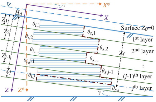
where γ is the slope angle [L/L]. The only difference between Equations (1) and (2) is that hydraulic conductivity K in the equation for the sloping scenario is replaced with K cos γ. This indicates that the effect of gravity normal to the surface direction is changed by cos γ (Chen and Young 2006, Mollerup and Hansen 2012, Muntohar et al. 2013). For small slope angle conditions in this study, we use this same slope factor cos γ of hydraulic conductivity for sloping soils. Similarly, the gravity term in the Richards equation is also changed by a factor cos γ in the HYDRUS-1D simulations (Šimůnek et al. 2013).

Assuming a saturated upper boundary condition with small slope angle, we obtain the infiltration rate when the wetting front is in the first top layer, i.e. Z_f ≤ Z₁:

(3)

in which i is the infiltration rate at any given time t, Z_f is the depth of the wetting front below the sloping surface, Z₀ is the depth of the surface, which is set to zero in this study, Z₁ is the depth of Layer 1, and H₀ and H_f are the hydraulic heads at the surface and the wetting front, respectively. Similar to the modification of gravity to a sloping surface, the overland flow head is h_p = H_d cos γ, where H_d is the overland flow depth normal to the surface, K_e,₁ is the effective hydraulic conductivity of Layer 1, K_e,₁ = cK_s,₁, and h_s,₁ is the capillary suction head at the wetting front of Layer 1. For any layer j, the capillary suction head is determined by (Neuman 1976, Ahuja 1983, Smith et al. 2002):

(4)

where h_i,_j and K_i,_j are, respectively, the soil water pressure head and hydraulic conductivity corresponding to the initial soil water content of layer j, and K_s,_j is the saturated hydraulic conductivity of layer j. In this study, we use the van Genuchten model (Van Genuchten 1980) to describe the hydraulic properties of soils, although any other forms could be adopted. The hydraulic properties are described by the following functions (Mualem 1976, Van Genuchten 1980):

(5)

(6)

(7)

(8)

where S_e is the dimensionless effective saturation, h is the pressure head [L], θ_r is the residual water content, θ_s is the saturated water content, K_r is the dimensionless relative hydraulic conductivity, and K is the hydraulic conductivity. The empirical parameters α [1/L], n and m determine the shape of the hydraulic conductivity function. , with n > 1.

The cumulative infiltration depth, I, is:

(9)

Since the infiltration rate i is given by dI/dt, the velocity of the advection wetting front in Layer 1 can be obtained by combining Equations (3) and (9):

(10)

By integrating Equation (10), we can determine the travel time of the wetting front from the surface to Z_f within the top Layer 1:

(11)

For the wetting front located in Layer 2, i.e. Z₁ < Z_f ≤ Z₂, the wetting front velocities at the interface between Layer 1 and Layer 2 should be the same, i.e. i = v₁ = v₂. Applying Darcy’s law at the interface between these two layers leads to:

(12)

Solving for H₁, Equation (12) gives:

(13)

where H_f is the hydraulic head at the wetting front within Layer 2, , and H₀ = h_p is the hydraulic head at the sloping surface. Then the infiltration rate can be determined as:

(14)

The cumulative infiltration at the wetting front Z_f is:

(15)

Since , we have

(16)

Integrating from depth Z₁ to Z_f to calculate the travel time, we have:

(17)

(18)

where t₁ is the travel time when the wetting front passes the interface between Layer 1 and Layer 2.

For the wetting front located in Layer j, i.e. Z_j−1 < Z_f ≤ Z_j:

(19)

(20)

(21)

where t_j−1 is the travel time when the wetting front passes the interface between Layer j – 1 and Layer j.

Equation (19) indicates that a stepwise change in the infiltration rate may occur when water passes the interface between layers n – 1 and layer n if the suction heads are different in these two layers:

(22)

and the infiltration rate when water arrives just below layer n – 1 (i.e. Z_f = Z_n−1) is:

(23)

The only difference between Equations (22) and (23) is the suction head h_s,n−1 and h_s,n. Therefore, a stepwise increase of infiltration rate occurs when the wetting front arrives at a soil layer with larger suction head than the previous layer. This stepwise increase is likely not possible and is caused by the assumption of instantaneous hydraulic equilibrium at the interface. The increase in the infiltration rate should be gradual when the wetting front passes the interface from a finer layer to a coarser layer under natural conditions.

2.2 Evaluation of the adjusting conductivity factor c

The effective hydraulic conductivity K_e is a key parameter in the GASLS model. To properly apply the value of K_e, we try to determine the adjusting factor for the hydraulic conductivity, c (=K_e/K_s) for various soil profile formations and infiltration conditions. The globally convergent shuffled complex evolution algorithm (SCE-UA) (Duan et al. 1992) is used to optimize the factor c in conjunction with the Richards equation numerical solver HYDRUS-1D (Šimůnek et al. 2008, 2013). The modified Richards equation, shown as Equation (24) with the same slope factor cos γ, is solved in the form:

(24)

and the results are used to optimize the adjusting factor c in the GASLS model. In Equation (24), γ = 0° applies for vertical flow, and γ = 90° for horizontal flow. The following initial and boundary conditions are used:

initial condition:

(25)

upper boundary condition:

(26)

lower boundary condition:

(27)

where h_i(z) is the initial water pressure head.

For most applications with practical significance, we are concerned about total infiltration and the infiltration rate in water budget considerations. As predicted by the HYDRUS-1D simulations, not all layers are saturated depending on the layer formation when the infiltration into the soil profile reaches a steady state. We can obtain the water amount infiltrated into the soil profile W_hy at steady state. Then the travel time t_hy from HYDRUS-1D is determined as the time when the cumulative infiltration depth is equal to the water amount W_hy. Since the GASLS model assumes fully saturated water content behind the wetting front, the travel time t_ga(c) with an adjusting factor c is the travel time when the GASLS cumulative infiltration depth W_ga equals the water amount W_hy. If HYDRUS-1D predicts a not fully saturated soil profile at steady state, the GASLS wetting front advances to an effective depth instead of the bottom of the soil profile to ensure an identical infiltration amount at the same time. The objective function in the inverse algorithm of SCE-UA is to minimize the difference between the HYDRUS-1D time t_hy and the GASLS model time t_ga by varying the factor c:

(28)

3 Results and discussion

3.1 Adjusting hydraulic conductivity factor c

To evaluate the optimal adjusting factor c for the GASLS model, five types of soils with contrasting textures are used to construct the layered formation. The hydraulic parameters of the five soil types are listed in Table 1 (Carsel and Parrish 1988, Wang et al. 2014). The optimal factor c is determined under a combination of varying soil types, layered formations, soil profile thicknesses, surface overland flow heads, and slope angles. For easy reference, the soil formations are expressed using abbreviations in the form {layer number}-{soil type from top to bottom} {total depth of soil profile}. For example, 4-BADC 200 means four layers with equal thickness of 50 cm of loamy sand, loam, sand and silt loam from top to bottom in a 200-cm soil profile, and 20-ABCD… 20 indicates 20 layers with equal thickness (five quaternary units) in a 20-cm soil profile.

Table 1. The van Genuchten hydraulic parameters of soils used in establishing guidelines to estimate the hydraulic conductivity adjusting factor c.

ID	Soil	θr	θs	θi	α (1/cm)	n	Ks (cm/min)	hs (cm)
A	Loam	0.078	0.430	0.150	0.036	1.560	0.017	6.926
B	Loamy sand	0.057	0.410	0.130	0.124	2.280	0.243	3.855
C	Silt loam	0.067	0.450	0.180	0.020	1.410	0.008	8.969
D	Sand	0.045	0.430	0.110	0.145	2.680	0.495	3.816
E	Loamy sand II	0.057	0.410	0.150	0.020	4.100	0.243	37.821

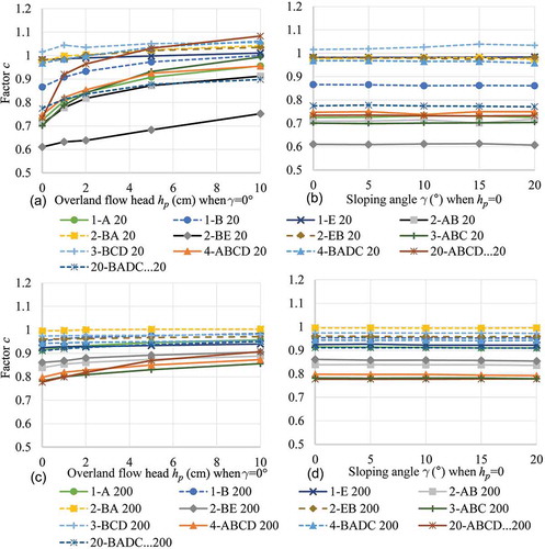
Figure 2 shows the optimal adjusting factor c for 234 scenarios. Figure 2(a) and (c) indicates that c increases with increasing overland flow depth for all soil formations. A significant increase in c is clearly shown with increasing overland flow head for fine soils or fine soil on top layered formations, while the effect of overland flow head on factor c is relatively insignificant for coarse soils or coarse soil on top formations. Factor c for coarse soils or coarse soil on top formations is close to 1 when the overland flow head is zero. Factor c for a single coarser soil profile is closer to 1 and larger than that for a finer soil profile. For example, the c values are 0.725, 0.866 and 0.982 for Loam, Loamy sand and Loamy sand II, respectively, in the 20-cm soil with h_d = 0, γ = 0° (see 1-A 20, 1-B 20 and 1-E 20 in Fig. 2(a)). In some layered formations, factor c may be larger than 1 with a large overland flow head. In general, the results demonstrate that c increases with increasing overland flow depth (from Fig. 2(a) and (c)). The comparison of same-layered formations for the 20-cm and 200-cm soil profiles illustrates that the change in c with overland flow depth is more significant in the 20-cm profile. For example, c increases from 0.725 to 0.956 for the 20-cm single loam soil (i.e. 1-A 20, Fig. 2(a)) when the overland flow depth increases from 0 to 10 cm, while for the 200-cm soil (i.e. 1-A 200, Fig. 2(c), c increases from 0.914 to 0.957. This can be explained by the fact that the effect of overland depth decreases as the thickness of the soil profile increases. Figure 2(b) and (d) shows that c is not affected by changing slope angle, which demonstrates that the same effective K_e as horizontal soil formations can be similarly used in dealing with sloping layered formations.

Figure 2. Influence of overland flow head h_p (a and c) and slope angle γ (b and d) on the optimal factor c for 20-cm (a and b) and 200-cm (c and d) soil profiles for layered formations under various scenarios. Abbreviations in the legends follow the format {layer number}-{soil type from top to bottom} {total depth of soil profile}.

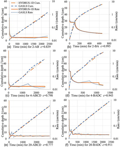
Figure 3 shows the infiltration results for six scenarios in the 200-cm profile with the determined optimal factor c. The results demonstrate that the GASLS model simulates an infiltration rate change when the wetting front passes the interface of soil layers, both from coarse to fine or from fine to coarse layers. Figure 3(b) shows that the HYDRUS-1D and GASLS results are in excellent agreement, and both indicate the infiltration rate is decreasing when the water advances to the bottom finer layer. Figure 3(e) and (f) shows that the infiltration process in a 20-layer soil tends to behave similarly to a homogeneous soil formation. In contrast to the HYDRUS-1D simulation results, the GASLS model can capture the infiltration rate changes when water advances into every soil layer. Both models indicate that the total travel time is shorter with coarse soil on top than fine soil on top formations. The optimal factor c decreases with a more heterogeneous soil profile. For example, Figure 3(a), (c) and (e) shows that c for two, four and 20 layers with finer soil on top is 0.839, 0.798 and 0.777, respectively. Figure 3(b), (d) and (f) indicates that a coarser soil on top formation has a larger factor c compared to Figure 3(a), (c) and (e). The cumulative infiltration depth at the final time from Figure 3(a) is smaller than that from Figure 3(b). The main reason is that the bottom coarse layer in Figure 3(a) is not fully saturated when the infiltration reaches a steady state. Comparison of cumulative infiltration depth from different soil layer arrangements in Figure 3 shows the bottom coarser layer is not fully saturated in the scenarios (i.e. Fig. 3(a), (c) and (e)), with the bottom coarser layer being below a finer soil layer. For these partial saturation scenarios, the sharp front GASLS model predicts an effective wetting front depth such that the total cumulative water infiltration amount equals that from the HYDRUS-1D at the steady state.

Figure 3. Cumulative infiltration depth and infiltration rate as a function of time for the 200-cm profile with h_d = 0, γ = 0° and optimal factor c.

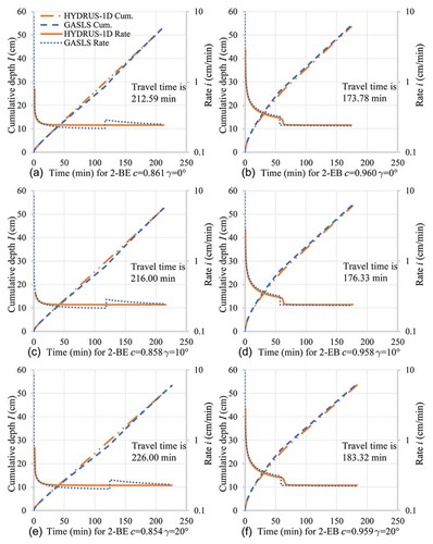
Figure 4 shows the infiltration processes in sloping two-layer soils with the optimal factor c when the overland flow head is zero. The results confirm that c is not affected by the slope angle, while the steady infiltration rate decreases and the travel time increases with increasing slope angle. For sloping soils with a coarser layer on top (i.e. Fig. 4(b), (d) and (f)), the GASLS model and HYDRUS-1D predictions are similar, and both capture the infiltration rate decrease when water passes the second finer layer. The results from the 2-BE case indicate that the GASLS model predicts an infiltration rate increase due to the larger suction in the bottom layer.

Figure 4. Cumulative infiltration depth and infiltration rate as a function of time in the sloping layered formation for the 200-cm profile with h_d = 0 and optimal factor c.

3.2 Comparison of GASLS model with experimental data in layered soils

3.2.1 Two-layer infiltration testing

First, we compare the GASLS model with the laboratory infiltration tests in two-layer soil columns conducted by Mohammadzadeh-Habili and Heidarpour (2015). The set-up and hydraulic parameters are shown in Table 2. All the experiments were performed in initially dry soils, i.e. . The soil formation in Test 1 has the coarser soil on top according to the saturated hydraulic conductivity, which is similar to the 2-BA case in our earlier discussion. Since the overland head is 2.7 cm and total thickness of soil profile is 53.4 cm, we may estimate c using the average of the optimal factors c of the 2-BA 20 and 2-BA 200 cases when h_p = 2 cm (i.e. c = (1.003 + 1.000)/2 = 1.002). For Test 2 with finer soil on top and large suction head soil in the bottom layer, we may estimate c for Test 2 as the average of the optimal factors c of 2-BE 20 and 2-BE 200 cases when h_p = 5 cm (i.e. c = (0.683 + 0.892)/2 = 0.788).

Table 2. Physical properties and hydraulic parameters in the two-layer tests (after Mohammadzadeh-Habili and Heidarpour 2015).

Test no.	Layer	hp (cm)	hs (cm)	Layer thickness (cm)	θr	θs	Ks (cm/min)	α (1/cm)	n
Test 1	Top	2.70	9.284	30.65	0.018	0.450	0.456	0.033	1.7
	Bottom		2.807	22.75	0.110	0.482	0.007	0.025	1.2
Test 2	Top	4.20	9.284	26.05	0.018	0.456	0.496	0.033	1.7
	Bottom		17.976	26.10	0.009	0.412	1.540	0.034	3.1

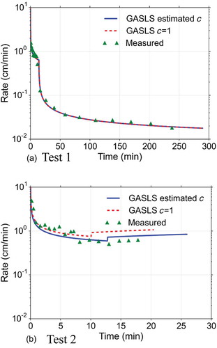
Figure 5 shows the comparison of the infiltration rate between the two-layer tests and the GASLS model with both the estimated factor c above and a convenient value of c = 1. Figure 5(a) demonstrates that both the estimated factor c (i.e. 1.002) and c = 1 are in good agreement with the measured infiltration rate data, with the root mean square error (RMSE) and coefficient of determination of 0.093 cm/min and 0.979, respectively. Since our estimated c (1.002) is virtually the same as 1, assigning factor c close to 1 is acceptable for the coarse layer on top formations. However, the simulation results in Test 2 with fine soil on top show that the GASLS with estimated factor c is better than that with c = 1, with RMSEs of 0.857 and 0.957 cm/min and R² of 0.705 and 0.693, respectively. However, the performance of GASLS to simulate Test 2 is not as good as that for Test 1. The laboratory data indicate that the infiltration rate decreased in the bottom coarse layer. Mohammadzadeh-Habili and Heidarpour (2015) illustrated that the unusual infiltration rate decrease in the bottom coarse layer was caused by the large air-filled volume in the experiments. The interaction between the low available water from the top finer soil and the large wetting front advancing rate in the bottom coarser soil resulted in entrapped air. Even so, the GASLS model based on the estimated c can still simulate the infiltration better than using simply c = 1.

Figure 5. Comparison of the infiltration rate in the two-layer soil formation between the measured data and the results from the GASLS model with different factor c: (a) Test 1 with estimated c = 1.002; and (b) Test 2 with estimated c = 0.788.

3.2.2 Three-layer infiltration testing

Wang et al. (2014) conducted constant 2-cm ponding infiltration experiments in three-layer soils with loams on top and at the bottom and a coarse sand layer in between. The thickness of the top, interlayer and bottom layer is 22.5, 20 and 17.5 cm, respectively. The layered formation is the same for the two tests, except for the interlayer of sand: in Test 1, Sand I is the interlayer, while Sand II is the interlayer in Test 2. The parameters are listed in Table 3. Since the suction heads of the two soils are large relative to the thickness of their layers, we may estimate the factor c based on the above 2-BE case and use the average of the optimal factors c of the 2-BE 20 and 2-BE 200 cases when h_p = 2 cm (i.e. c = (0.638 + 0.880)/2 = 0.759). This estimation ignores the bottom layer because it is involved in a transformation from coarser soil to finer soil, which has a relatively insignificant influence on c. Since the Sand II soil in Test 2 has a significantly larger suction head compared to Sand I, we use a slightly larger value of 0.789 for c.

Table 3. Hydraulic parameters of the three-layer tests (after Wang et al. 2014).

Soil	θr	θs	θi	α (1/cm)	n	Ks (cm/min)	hs (cm)
Loam	0.014	0.400	0.080	0.009	1.58	0.057	28.644
Sand I	0.010	0.275	0.065	0.050	2.50	0.160	10.536
Sand II	0.005	0.300	0.020	0.018	4.30	0.220	39.875

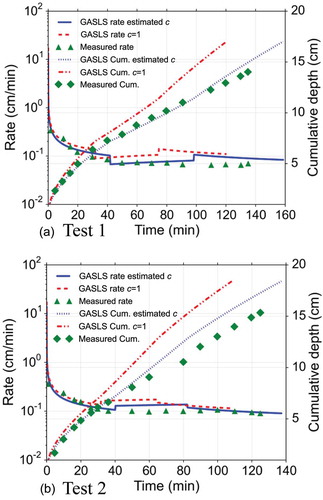
Figure 6(a) demonstrates that the GASLS with estimated c agrees with measured data, and is significantly better than that with c = 1. The infiltration rate RMSE and R² of the GASLS with estimated c (0.759) are 0.028 cm/min and 0.902, respectively. The cumulative infiltration depth RMSE and R² of GASLS with estimated c are 0.443 cm and 0.992, respectively. Both the measurements and the GASLS model show an infiltration rate decrease in the second interlayer due to its lower suction head, which is consistent with the study of Eisenhauer et al. (1992). For Test 2, shown in Figure 6(b), the GASLS with estimated c shows a good agreement with the measured data, and is significantly better than that with c = 1. The infiltration rate RMSE and R² of the GASLS with estimated c are 0.062 cm/min and 0.831, respectively, and the cumulative infiltration depth RMSE and R² of the GASLS with estimated c are 1.156 cm and 0.994, respectively. The infiltration rate increase in the second interlayer with coarse soil and decrease in third bottom layer predicted by the GASLS may be observed in the measurements. The coarser Sand II in the interlayer has larger saturated hydraulic conductivity and suction head than those of the top and bottom loam soils. The significantly larger suction in the interlayer coarser Sand II leads to a considerably larger rate. The infiltration rate increase when the water advances in the Sand II interlayer is in agreement with Wang et al. (2014). Ma et al. (2011) also demonstrated a possible infiltration rate increase when water flows from a fine layer into a coarse layer from both experimental observations and modelling simulations. However, the small stepwise increase from the GASLS model is a result of the assumption of instantaneous hydraulic equilibrium at the interface, which should be gradual under natural conditions.

Figure 6. Comparison of the infiltration rate and the cumulative infiltration depth in the three-layer soil formation between the measured data and results from the GASLS model with different factor c: (a) Test 1 with estimated c = 0.759; and (b) Test 2 with estimated c = 0.789.

3.2.3 Multi-layer infiltration testing

In this multi-layer infiltration test, we evaluate the GASLS model using the field double-ring infiltrometer measurement data from two sites, SV10 and SV62, conducted by Huang et al. (2011) and Zettl et al. (2011). The natural soil profiles in the two sites are vertically heterogeneous and coarse contents are very high. Soils profiles are complicated, with as many as 16 layers of contrasting hydraulic properties, as shown in Table 4. The overland head in the test was maintained at about 10 cm. According to the variability in K_s, site SV10 is less heterogeneous with smaller standard deviation and SV62 is much more heterogeneous with larger standard deviation. For the SV10 site, the total thickness of the soil profile is 110 cm, with 14 layers having relatively homogeneous hydraulic conductivities. We estimate factor c using the average of optimal factors of the 1-B 20 and 1-B 200 cases when h_p = 10 cm, i.e. c = (1.000 + 0.984)/2 = 0.992. For the SV62 site, it can be considered as a two-layer soil profile with finer soil on top, since there was a 40-cm finer sand layer overlying a medium sand layer. Thus we may estimate c using the average of the optimal factors of the 2-AB 20 and 2-AB 200 cases when h_p = 10 cm, i.e. c = (0.912 + 0.888)/2 = 0.900. The initial water contents are not uniform in this field case. To represent this non-uniformity in the initial water contents, we treat the soil profile as consisting of many layers in the GASLS model, 110 layers for the SV10 site and 100 layers for the SV62 site to be specific.

Table 4. Hydraulic parameters for test sites SV10 and SV62 (after Huang et al. 2011). SD: standard deviation.

Layer	Depth (cm)	θr	θs	α (1/cm)	n	Ks (cm/min)	Avg. θi	Avg. hs (cm)
SV10
1	0–8	0.017	0.500	0.228	3.235	2.378	0.018	2.750
2	8–14	0.016	0.500	0.172	3.195	1.985	0.020	3.619
3	14–18	0.019	0.500	0.142	3.511	2.093	0.026	4.616
4	18–24	0.025	0.492	0.124	2.993	1.710	0.036	4.820
5	24–30	0.028	0.420	0.134	2.684	1.693	0.044	4.125
6	30–40	0.007	0.417	0.128	2.630	1.663	0.047	4.250
7	40–46	0.001	0.427	0.098	3.602	1.761	0.046	6.777
8	46–60	0.000	0.392	0.096	3.605	1.616	0.054	6.925
9	60–70	0.000	0.418	0.106	3.653	1.855	0.047	6.309
10	70–80	0.000	0.374	0.084	3.608	1.546	0.045	7.916
11	80–86	0.000	0.393	0.076	3.641	1.670	0.045	8.789
12	86–94	0.000	0.393	0.084	3.638	1.566	0.050	7.949
13	94–100	0.000	0.411	0.086	3.644	1.630	0.050	7.769
14	100–110	0.000	0.430	0.078	3.551	1.535	0.051	8.457
Mean		0.008	0.433	0.117	3.371	1.764	0.041	6.077
SD		0.011	0.045	0.043	0.365	0.240	0.012	2.000
SV62
1	0–6	0.000	0.467	0.258	1.986	0.620	0.041	1.556
2	6–15	0.000	0.300	0.216	1.875	0.216	0.022	1.702
3	15–27	0.000	0.379	0.102	2.296	0.470	0.037	4.703
4	27–32	0.000	0.388	0.228	1.736	0.719	0.041	1.403
5	32–37	0.000	0.389	0.186	2.070	0.576	0.051	2.285
6	37–42	0.000	0.405	0.19	1.994	0.554	0.067	2.126
7	42–46	0.000	0.400	0.304	2.044	0.505	0.057	1.375
8	46–54	0.000	0.324	0.352	1.711	1.311	0.043	0.882
9	54–60	0.000	0.311	0.238	1.955	0.750	0.042	1.649
10	60–67	0.000	0.305	0.202	1.982	0.789	0.042	1.982
11	67–71	0.005	0.302	0.198	1.931	1.059	0.042	1.945
12	71–78	0.005	0.305	0.21	1.970	1.865	0.042	1.890
13	78–81	0.005	0.302	0.21	1.851	2.109	0.042	1.714
14	81–88	0.003	0.289	0.212	1.997	2.636	0.042	1.909
15	88–97	0.004	0.316	0.214	2.019	1.901	0.042	1.920
16	97–100	0.004	0.332	0.218	2.024	1.268	0.042	1.891
Mean		0.002	0.345	0.221	1.965	1.084	0.043	1.933
SD		0.002	0.052	0.054	0.135	0.701	0.009	0.811

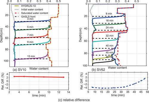
Figure 7 shows the infiltration results from the GASLS model with estimated c and c = 1. For the SV62 test, the cumulative infiltration depth simulated with the GASLS over-predicts the data measured by the inner ring. Huang et al. (2011) indicated that there were lateral flows from the outer ring to the inner ring. Since the estimated factor c (0.992) based on the guidelines we established earlier (Fig. 2) is very close to 1, it is not a surprise to see that the cumulative infiltration results from c = 1 are also close to those for the estimated c. Given the uncertainty and errors in the ring measurements, the simulation results from the GASLS are reasonable for both the sites SV10 and SV62. Figure 8 shows the results of water content profiles at sites SV10 and SV62 from the GASLS simulations with estimated c, as well as those from the HYDRUS-1D simulations. As expected, the water content profiles from the GASLS are a sharp wetting front in the range of the wetting front curve from the HYDRUS-1D simulations. The agreement with the HYDRUS-1D simulations in Figure 8(a) is better than that in Figure 8(b), since the soil profile in the SV62 site is more heterogeneous than that in the SV60 site. Even so, the wetting front with the GASLS model using estimated c is in the range of the wetting front simulated by HYDRUS-1D. Since the SV62 site soil profile in Figure 8(b) can be considered as a two-layer formation with finer soil on top, the estimated factor c is less than 1, and the soil profile in the bottom part is not saturated as predicted by HYDRUS-1D. Although the factor c leads to slight underestimation of infiltration amount when the wetting front is in the upper part of the soil profile, the relative differences in cumulative infiltration are always less than 5%, which demonstrates that the GASLS model with estimated factor c can reasonably predict the total infiltration amount.

Figure 7. Comparison of the infiltration rate and the cumulative infiltration depth in the multi-layer soil formation between the measured data and the results from the GASLS model: (a) SV10 test with estimated c = 0.992; and (b) SV62 test with estimated c = 0.900.

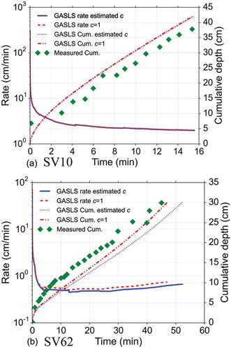
Figure 8. Dynamics of the water content profiles in the multi-layer soils using the GASLS model with estimated factor c and HYDRUS-1D: (a) SV10 test with c = 0.992; (b) SV62 test with c = 0.900; and (c) relative difference of cumulative infiltration between the simulations of the GASLS and HYDRUS-1D models.

3.3 Comparison of GASLS model with experimental data in sloping soil surface

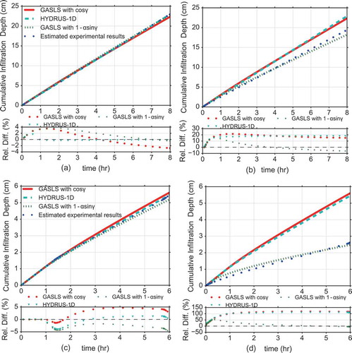
Since the gravity effects on infiltration decrease with slope angle by a factor of cos γ, several studies (e.g. Philip 1991, Chen and Young 2006, Essig et al. 2009, Haghizadeh et al. 2014) have examined whether the same factor also applies to infiltration. Morbidelli et al. (2015, 2016) recently conducted two laboratory studies of infiltration on sloping surfaces with slope angle from 1° to 15° under steady rainfall. The two experiments were similar, with a loam soil overlying a gravel layer, one with a grassy surface under 8-h duration rainfall and the other with bare soil under 6-h duration rainfall. We extend the GASLS model to simulate the infiltration process under steady rainfall condition such that we can compare the results with these two experiments. We first determine the cumulative infiltration depth and cumulative runoff based on the results of Morbidelli et al. (2015, 2016), and then estimate the soil parameters using the HYDRUS-1D by minimizing the difference between the results of simulation and experiments. The factor c in the GASLS model is estimated as 0.91 for the two loam soils based on the similarity of the soils and infiltration set-ups between Scenario 1-A in Figure 2 and the experiments.

Figure 9(a) and (c) shows the relative differences of cumulative infiltration depth compared with the experiments. Both the GASLS and HYDRUS-1D models agree well with the experimental results for the nearly horizontal surface, with γ = 1º, with less than 5% relative differences. The estimated factor c = 0.91 is suitable for the two experiments with insignificant differences when comparing the HYDRUS-1D and experimental results. The GASLS model simulation with estimated factor is better than that with c = 1, especially with bare soil (Fig. 9(c)). For the infiltration processes on the sloping soil surface with γ = 5º (Fig. 9(b) and (d)), both the GASLS and HYDRUS-1D models using the factor cos γ overestimate the cumulative infiltration compared to the experimental results, which is consistent with the results of Morbidelli et al. (2015) that the magnitudes of the infiltration reduction with slope are much larger than those using the factor cos γ. The experimental results also demonstrate that the ratio of cumulative runoff over cumulative infiltration is significantly larger in bare soil than grassy soil, which is consistent with the findings of Hino et al. (1987) and Pan and Shangguan (2006). This is not fully captured by the GASLS and HYDRUS-1D, which do not take the surface roughness into account in examining the slope effects. Since the agreement between the GASLS simulations and experimental results is better in grassy soil (K_s = 2.87 cm/h) than in bare soil (K_s = 0.815 cm/h), we may conclude that the GASLS model with the factor cos γ is more applicable for soils with greater surface roughness and larger hydraulic conductivity. As discussed in the Introduction, there have been many studies suggesting that an adjusting factor other than cos γ might be more appropriate in accounting for the slope effects. We also perform additional simulations using the gravity reduction factor 1 – α sin γ instead of cos γ and K_e = K_s(1 – α sin γ), as proposed by Essig et al. (2009). The results based on the factor 1 – α sin γ are also shown in Figure 9. The values of parameter α are calculated as 1.834 and 5.952, respectively, for grassy soil and bare soil, by the measured steady deep flow K_e from Morbidelli et al. (2015, 2016). The results show that the GASLS with 1 – α sin γ lead to more reasonable comparison, especially for the bare soil experiments, than the factor cos γ for both the GASLS and HYDRUS-1D simulations. The introduction of the additional parameter α increases the flexibility of correction for slope effects and effective hydraulic conductivity, which can better simulate the significant reduction of infiltration on a sloping surface. In general, the slope factor is used to approximate multi-dimensional infiltration in a sloping surface by one-dimensional flow, which may introduce errors to a certain degree. Note that the developed GASLS model can easily accommodate any slope adjusting factor.

Figure 9. Comparison of infiltration processes from the GASLS model, HYDRUS-1D model and laboratory experiments: (a and b) for grassy soil with γ = 1° and γ = 5°, respectively, compared to Morbidelli et al. (2016); (c and d) for bare soil with γ = 1° and γ = 5°, respectively, compared to Morbidelli et al. (2015). The values of α in 1 – α sin γ are 1.834 and 5.952 for grassy soil and bare soil, respectively.

4 Summary and conclusions

In this study, we developed a modified sharp wetting front infiltration model, GASLS, to simulate infiltration processes through sloping layered soil formations. The adjusting conductivity factor c, i.e. the ratio of the effective hydraulic conductivity to the saturated hydraulic conductivity, is a key parameter in the model. We developed guidelines to estimate factor c, which is the same for all individual layers, based on comparisons with the numerical solution of the Richards equation performed through the HYDRUS-1D solver under 234 scenarios with different soil formations, soil types, overland flow heads and slope angles. The results from experiments in the literature are explored to compare and validate the GASLS model.

The proposed GASLS model can reasonably describe infiltration processes in a sloping layered formation with an appropriate factor c. The model can simulate the infiltration in layered soils with non-uniform initial water contents in individual layers and under steady rainfall.

The adjusting conductivity factor c varies with soil type, soil formation and infiltration conditions. However, one major conclusion is that c is not affected by the slope of the layered formation to any significant extent.

General guidelines were established to estimate the factor c so the model can be used to simulate the infiltration into a layered sloping soil formation with reasonable accuracy. The factor c increases and approaches 1 with increases in the depth of the soil profile and the overland flow head. For fine soils, or layered formations with finer soils on top of the profile, the c is much smaller than 1. The factor c for coarse soils, or layered formations with coarse soils on the top, is close to 1. The ratio of the soil suction head over the overland flow head as well as the length of the soil profile also affect the value of c.

The infiltration wetting front in sloping layered soil formations is delayed, with longer travel time compared to the same profile without a slope. Comparison with laboratory experiments on a sloping surface indicates that the GASLS model with a slope factor of cos γ overestimates infiltration and suggests that the GASLS model with factor 1 – α sin γ can better represent the effects of a sloping surface. The GASLS model can incorporate any slope adjusting factor.

Acknowledgements

The authors are thankful to the editors and anonymous reviewers for their valuable suggestions and comments which helped to improve the manuscript.

Disclosure statement

No potential conflict of interest was reported by the authors.

Additional information

Funding

This research was supported by the Engineering Initiative program at the University of Wyoming. This work was also partially supported by the Wyoming Center for Environmental Hydrology and Geophysics (WyCEHG) funded by NSF EPS-1208909.

References

- Ahuja, L.R., 1983. Modeling infiltration into crusted soils by the Green–Ampt approach. Soil Science Society of America Journal, 47, 412–418. doi:10.2136/sssaj1983.03615995004700030004x
- Arnold, J.G., et al., 2012. Soil & water assessment tool: input/output documentation. Temple, TX. Available from: http://swat.tamu.edu/media/69296/SWAT-IO-Documentation-2012.pdf
- Assouline, S., 2013. Infiltration into soils: conceptual approaches and solutions. Water Resources Research, 49 (4), 1755–1772. doi:10.1002/wrcr.20155
- Bouwer, H., 1966. Rapid field air entry value and parameters. Water Resources Research, 2 (4), 729–738. doi:10.1029/WR002i004p00729
- Cameira, M.R., et al., 2000. Evaluating field measured soil hydraulic properties in water transport simulations using the RZWQM. Journal of Hydrology, 236 (1–2), 78–90. doi:10.1016/S0022-1694(00)00286-9
- Carsel, R.F. and Parrish, R.S., 1988. Developing joint probability distributions of soil water retention characteristics. Water Resources Research, 24 (5), 755–769. doi:10.1029/WR024i005p00755
- Chen, L. and Young, M.H., 2006. Green-Ampt infiltration model for sloping surfaces. Water Resources Research, 42 (7), 1–9. doi:10.1029/2005WR004468
- Chu, X. and Mariño, M.A., 2005. Determination of ponding condition and infiltration into layered soils under unsteady rainfall. Journal of Hydrology, 313 (3–4), 195–207. doi:10.1016/j.jhydrol.2005.03.002
- Corradini, C., Melone, F., and Smith, R.E., 2000. Modeling local infiltration for a two-layered soil under complex rainfall patterns. Journal of Hydrology, 237 (1–2), 58–73. doi:10.1016/S0022-1694(00)00298-5
- Damodhara, R.M., Raghuwanshi, N.S., and Singh, R., 2006. Development of a physically based 1D-infiltration model for irrigated soils. Agricultural Water Management, 85 (1–2), 165–174. doi:10.1016/j.agwat.2006.04.009
- Dorofki, M., et al., 2014. A GIS-ANN-Based approach for enhancing the effect of slope in the modified Green-Ampt model. Water Resources Management, 28 (2), 391–406. doi:10.1007/s11269-013-0489-7
- Duan, Q., Sorooshian, S., and Gupta, V., 1992. Effective and efficient global optimization for conceptual rainfall-runoff models. Water Resources Research, 28 (4), 1015–1031. doi:10.1029/91WR02985
- Eisenhauer, D.E., Heermann, D.F., and Klute, A., 1992. Surface sealing effects on infiltration with surface irrigation. Transactions of the ASAE, 35 (6), 1799–1807. doi:10.13031/2013.28799
- Essig, E.T., et al., 2009. Infiltration and deep flow over sloping surfaces: comparison of numerical and experimental results. Journal of Hydrology, 374 (1–2), 30–42. doi:10.1016/j.jhydrol.2009.05.017
- Flanagan, D.C., Gilley, J.E., and Franti, T.G., 2007. Water Erosion Prediction Project (WEPP): development history, model capabilities, and future enhancements. Transactions of the ASABE, 50 (5), 1603–1612. doi:10.13031/2013.23968
- Fox, D.M., Bryan, R.B., and Price, A.G., 1997. The influence of slope angle on final infiltration rate for interrill conditions. Geoderma, 80 (1–2), 181–194. doi:10.1016/S0016-7061(97)00075-X
- Gowdish, L. and Muñoz-Carpena, R., 2009. An improved Green–Ampt infiltration and redistribution method for uneven multistorm series. Vadose Zone Journal, 8 (2), 470. doi:10.2136/vzj2008.0049
- Green, W.H. and Ampt, G.A., 1911. Studies of soil physics, part I – the flow of air and water through soils. Journal of Agricultual Science, 4, 1–24.
- Haghizadeh, A., Soleimani, L., and Zeinivand, H., 2014. Optimization of the conceptual model of green-ampt using artificial neural network model (ANN) and WMS to estimate infiltration rate of soil (case study: kakasharaf watershed, Khorram Abad, Iran). Journal of Water Resource and Protection, 6, 473–480. doi:10.4236/jwarp.2014.65047
- Han, T., et al., 2014. Sensitivity analysis of cumulative infiltration and stability at different angles of unsaturated soil slope. Journal of Central South University (Science and Technology), 45 (5), 1583–1589.
- Hino, M., Fujita, K., and Shutto, H., 1987. A laboratory experiment on the role of grass for infiltration and runoff processes. Journal of Hydrology, 90 (3–4), 303–325. doi:10.1016/0022-1694(87)90073-4
- Huang, M., et al., 2011. Infiltration and drainage processes in multi-layered coarse soils. Canadian Journal of Soil Science, 91 (2), 169–183. doi:10.4141/cjss09118
- Huat, B.B.K., Ali, F.H.J., and Low, T.H., 2006. Water infiltration characteristics of unsaturated soil slope and its effect on suction and stability. Geotechnical and Geological Engineering, 24 (5), 1293–1306. doi:10.1007/s10706-005-1881-8
- Kidwell, M.R., Weltz, M.A., and Phillip, D., 1997. Estimation of Green-Ampt for rangelands hydraulic conductivity. Journal of Range Management, 50 (3), 290–299. doi:10.2307/4003732
- King, K.W., Arnold, J.G., and Bingner, R.L., 1999. Comparison of Green-Ampt and curve number methods on Goodwin Creek watershed using SWAT. American Society of Agricultural Engineers, 42 (4), 919–925. doi:10.13031/2013.13272
- Liu, G., Craig, J.R., and Soulis, E.D., 2011. Applicability of the Green-Ampt infiltration model with shallow boundary conditions. Journal of Hydrologic Engineering, 16 (3), 266–273. doi:10.1061/(ASCE)HE.1943-5584.0000308
- Liu, J., Zhang, J., and Feng, J., 2008. Green–Ampt model for layered soils with nonuniform initial water content under unsteady infiltration. Soil Science Society of America Journal, 72 (4), 1041. doi:10.2136/sssaj2007.0119
- Lv, T., et al., 2015. Determining permeability coefficient of Green-Ampt model for infiltration analysis. Rock and Soil Mechanics, 36 (Supp.1), 341–345. doi:10.16285/j.rsm.2015.S1.058
- Ma, D., et al., 2015. Derivation of the relationships between Green–Ampt model parameters and soil hydraulic properties. Soil Science Society of America Journal, 79 (4), 1030. doi:10.2136/sssaj2014.12.0501
- Ma, Y., et al., 2011. Water infiltration in layered soils with air entrapment: modified Green-Ampt model and experimental validation. Journal of Hydrologic Engineering, 16 (8), 628–638. doi:10.1061/(ASCE)HE.1943-5584.0000360
- Mishra, S.K., Tyagi, J.V., and Singh, V.P., 2003. Comparison of infiltration models. Hydrological Processes, 17 (13), 2629–2652. doi:10.1002/hyp.1257
- Mohammadzadeh-Habili, J. and Heidarpour, M., 2015. Application of the Green–Ampt model for infiltration into layered soils. Journal of Hydrology, 527, 824–832. doi:10.1016/j.jhydrol.2015.05.052
- Mollerup, M. and Hansen, S., 2012. Power series solution for ponded infiltration on sloping surfaces. Journal of Hydrology, 464–465, 431–437. doi:10.1016/j.jhydrol.2012.07.031
- Morbidelli, R., et al., 2011. Infiltration-soil moisture redistribution under natural conditions: experimental evidence as a guideline for realizing simulation models. Hydrology and Earth System Sciences, 15 (9), 2937–2945. doi:10.5194/hess-15-2937-2011
- Morbidelli, R., et al., 2015. Infiltration on sloping surfaces: laboratory experimental evidence and implications for infiltration modeling. Journal of Hydrology, 523, 79–85. doi:10.1016/j.jhydrol.2015.01.041
- Morbidelli, R., et al., 2016. Laboratory investigation on the role of slope on infiltration over grassy soils. Journal of Hydrology, 543, 542–547. doi:10.1016/j.jhydrol.2016.10.024
- Morbidelli, R., et al., 2014. Soil water content vertical profiles under natural conditions: matching of experiments and simulations by a conceptual model. Hydrological Processes, 28 (17), 4732–4742. doi:10.1002/hyp.9973
- Mualem, Y., 1976. A new model for predicting the hydraulic conductivity of unsaturated porous media. Water Resources Research, 12 (3), 513–522. doi:10.1029/WR012i003p00513
- Muntohar, A.S., Ikhsan, J., and Liao, H.J., 2013. Influence of rainfall patterns on the instability of slopes. Civil Engineering Dimension, 15 (2), 120–128. doi:10.9744/ced.15.2.120-128
- Neuman, S.P., 1976. Wetting front pressure head in the infiltration model of Green and Ampt. Water Resources Research, 12 (3), 564–566. doi:10.1029/WR012i003p00564
- Pan, C. and Shangguan, Z., 2006. Runoff hydraulic characteristics and sediment generation in sloped grassplots under simulated rainfall conditions. Journal of Hydrology, 331 (1–2), 178–185. doi:10.1016/j.jhydrol.2006.05.011
- Philip, J.R., 1991. Hillslope infiltration: planar slopes. Water Resources Research, 27 (1), 109–117. doi:10.1029/90WR01704
- Pirone, M., et al., 2015. Soil water balance in an unsaturated pyroclastic slope for evaluation of soil hydraulic behaviour and boundary conditions. Journal of Hydrology, 528, 63–83. doi:10.1016/j.jhydrol.2015.06.005
- Ribolzi, O., et al., 2011. Impact of slope gradient on soil surface features and infiltration on steep slopes in northern Laos. Geomorphology, 127 (1–2), 53–63. doi:10.1016/j.geomorph.2010.12.004
- Rossman, L.A., 2015. Storm water management model user’s manual. Version5.1. Cincinnati, OH: National Risk Management Laboratory Office of Research and Development U.S. Environmental Protection Agency.
- Sajjan, A.K., Gyasi-Agyei, Y., and Sharma, R.H., 2013. Rainfall–runoff modelling of railway embankment steep slopes. Hydrological Sciences Journal, 58 (5), 1162–1176. doi:10.1080/02626667.2013.802323
- Scharffenberg, W., 2015. Hydrologic modeling system user’s manual. Version4.1. Washington, DC: Hydrologic Engineering Center.
- Šimůnek, J., et al., 2013. The HYDRUS-1D software package for simulating the one-dimensional movement of water, heat, and multiple solutes in variably-saturated media. Version 4.17. HYDRUS Softw. Ser. 3. Riverside, CA: Department of Environmental Sciences, University of California, Riverside.
- Šimůnek, J., Van Genuchten, M.T., and Šejna, M., 2008. Development and applications of the HYDRUS and STANMOD software packages and related codes. Vadose Zone Journal, 7 (2), 587. doi:10.2136/vzj2007.0077
- Sinai, G. and Dirksen, C., 2006. Experimental evidence of lateral flow in unsaturated homogeneous isotropic sloping soil due to rainfall. Water Resources Research, 42 (12), 1–12. doi:10.1029/2005WR004617
- Smith, E., et al. 2002. Infiltration theory for hydrologic applications. In: Water resources monograph. Vol. 15. Washington, DC: American Geophysical Union. doi:10.1029/WM015
- Stewart, R.D., et al., 2013. Modeling effect of initial soil moisture on sorptivity and infiltration. Water Resources Research, 49 (10), 7037–7047. doi:10.1002/wrcr.20508
- Van den Putte, A., et al., 2013. Estimating the parameters of the Green–Ampt infiltration equation from rainfall simulation data: why simpler is better. Journal of Hydrology, 476, 332–344. doi:10.1016/j.jhydrol.2012.10.051
- van Genuchten, M.T., 1980. A closed-form equation for predicting the hydraulic conductivity of unsaturated soils. Soil Science Society of America Journal, 44 (5), 892. doi:10.2136/sssaj1980.03615995004400050002x
- Wang, C., Mao, X., and Hatano, R., 2014. Modeling ponded infiltration in fine textured soils with coarse interlayer. Soil Science Society of America Journal, 78 (3), 745. doi:10.2136/sssaj2013.12.0535
- Warrick, A.W., Wierenga, P.J., and Pan, L., 1997. Downward water flow through sloping layers in the vadose zone: analytical solutions for diversions. Journal of Hydrology, 192 (1–4), 321–337. doi:10.1016/S0022-1694(96)03080-6
- Xue, J. and Gavin, K., 2008. Effect of rainfall intensity on infiltration into partly saturated slopes. Geotechnical and Geological Engineering, 26 (2), 199–209. doi:10.1007/s10706-007-9157-0
- Zettl, J., et al., 2011. Influence of textural layering on field capacity of coarse soils. Canadian Journal of Soil Science, 91 (2), 133–147. doi:10.4141/cjss09117
- Zhang, J., et al., 2014. Probabilistic prediction of rainfall-induced slope failure using a mechanics-based model. Engineering Geology, 168, 129–140. doi:10.1016/j.enggeo.2013.11.005