Trend analysis using discrete wavelet transform (DWT) for long-term precipitation (1851–2006) over India

ABSTRACT

This study is an attempt to determine the trends in monthly, annual and monsoon total precipitation series over India by applying linear regression, the Mann-Kendall (MK) test and discrete wavelet transform (DWT). The linear regression test was applied on five consecutive classical 30-year climate periods and a long-term precipitation series (1851–2006) to detect changes. The sequential Mann-Kendall (SQMK) test was applied to identify the temporal variation in trend. Wavelet transform is a relatively new tool for trend analysis in hydrology. Comparison studies were carried out between decomposed series by DWT and original series. Furthermore, visualization of extreme and contributing events was carried out using the wavelet spectrum at different threshold values. The results showed that there are significant positive trends for annual and monsoon precipitation series in North Mountainous India (zone NMI) and North East India (NEI), whereas negative trends were detected when considering India as whole.

EDITOR A. Castellarin ASSOCIATE EDITOR S. Kanae

KEYWORDS:

• wavelet transform
• sequential Mann-Kendall test
• trend
• precipitation
• climate change

1 Introduction

There is enough evidence in recent studies (Meehl et al. 2007, Randall et al. 2007, Reeves et al. 2007, Meenu et al. 2013, Mehrotra et al. 2013, Pachauri et al. 2014) to confirm that the climate is warming. It is one of the main causes of intensification of the hydrological cycle. Climate variability affects the components of the hydrological cycle, in both quality and quantity (Pandey et al. 2017). It has been observed that atmospheric temperatures are rising and precipitation patterns are changing (Joos et al. 2001, Kahya and Kalaycı 2004, Dibike and Coulibaly 2005, Holman 2005, Gosain et al. 2006, Fowler et al. 2007, Barkhordarian et al. 2012, Sethi et al. 2015). Precipitation is one of the most important components of hydrological processes. The distribution of precipitation plays a key role in the development of any country and affects the water management systems in irrigation, power generation, agriculture productivity, and flood and drought monitoring (Zaveri et al. 2016, Ribbe et al. 2017).

In recent years, many methods have been introduced to analyse trends detected in precipitation time series (Lettenmaier et al. 1994, Lu 1997, Klein Tank and Können 2003, Kahya and Kalaycı 2004, Hamlet et al. 2007, Mekis and Vincent 2011, Duhan et al. 2013, Gocic and Trajkovic 2013, Vittal et al. 2013, Goyal 2014, Murumkar and Arya 2014). The purpose of understanding trends is to detect expected changes and uncertainty. There are various methods in the literature to analyse trend detection. Sonali and Kumar (2013) analysed the trend of maximum and minimum temperature in annual, monthly, winter, pre-monsoon, monsoon and post-monsoon periods for three time slots (1901–2003, 1948–2003 and 1970–2003) over India as a whole and over seven homogeneous regions. Considering the effect of serial correlation, trend detection analysis was performed using a variety of nonparametric methods. A rigorous analysis of trends and persistence in precipitation has been carried out over the three major river basins in the Himalayan region in India (Ganges, Brahmaputra and Meghna) by Mirza et al. (1998). These three river basins have been examined for trends using a variety of trend tests, namely the Mann-Kendall rank statistic test, Student’s t-test and regression analysis, and for persistence using first-order autocorrelation analysis. Goswami et al. (2006) used a daily rainfall dataset for India and detected significant rising trends in the extreme rain events. In Central India, they found a significant decreasing trend in the mean values of rainfall during the monsoon in the period 1951–2000. In their conclusion, the authors declared that in future a substantial increase in hazards related to flood is expected over Central India. Rahmani et al. (2015) analysed the daily precipitation for Kansas (USA) using statistical methods, such as the Mann-Kendall method, linear regression and the Spearman test, for trend detection. In their analysis of 23 stations, significant change points were detected, which is useful in managing the water resources system.

There are limited studies based on wavelet transform, a relatively new tool for trend detection studies. Wavelet transform is a very useful tool for the decomposition of time series into a small number of elementary series that are based on both time and frequency. Wavelet analysis has the capability to expose many characteristics of a time series, such as trends, periodicity, discontinuities and change points (Labat 2005, Partal and Küçük 2006, Sang et al. 2009, Nikhil Raj and Azeez 2012, Joshi et al. 2016). Adarsh and Janga Reddy (2015) investigated rainfall trends for southern India using nonparametric methods and a wavelet transform method. Sequential changes for annual and monsoon trends have also been analysed using the sequential Mann-Kendall (SQMK) test. Nalley et al. (2012) analysed trends in streamflow and precipitation for Canada using discrete wavelet transform (DWT) methods. The continuous wavelet transform was used by Tarhule et al. (2015) to analyse the variability of precipitation and streamflow. Their study was carried out on 100 years of data for northwestern Oklahoma, USA. The results showed variability in annual precipitation and streamflow. Xu et al. (2009) evaluated climate change impacts in the Tarim River basin in China using a decomposition and reconstruction technique based on wavelet transform. Climatic parameters such as annual temperature, precipitation and relative humidity were used to analyse the trend in time series.

In the recent past, many trend studies were based on long-term and short-term time series of different climatic and hydrological variables, e.g. precipitation, temperature and discharge. Hydrological variables exhibit substantial dependence over a wide range of temporal and spatial scales. The spatial variability of a hydrological variable may also have an effect on hydrological modelling. Therefore, the main objectives of this study are: (a) to carry out trend analysis using climatological categorization of time series (30 years) data, in addition to investigating general long-term trends (156 years) over all seven zones of India based on annual and monsoon precipitation; (b) to study temporal changes in trends for monthly, annual and monsoon precipitation to help derive changes in climatological time zones, as well as spatial variability of precipitation under Indian conditions; (c) to use a combination of the MK test with DWT to analyse trends in Indian long-term precipitation time series, in which monthly, annual and monsoon precipitation series are decomposed via DWT into approximation coefficient and detailed series using convolution of low-pass filter and high-pass filter. In order to identify the suitable mother wavelet and decomposed level, the criteria proposed by Nalley et al. (2012) were used to decompose the original series; (d) to apply the SQMK test to the original series and a combination of approximation and detailed series in order to check the trend and periodicity of the series; and (e) to derive a visualization of extreme events and contributing events at different threshold values.

2 Study area and data collection

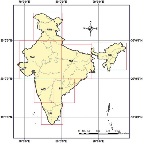
In this study, DWT was applied to detect the trend of precipitation for India. The country was divided into seven zones for the study, considering the monsoon and annual precipitation data within each of these zones to be homogeneous. The seven zones, shown in Figure 1, are North Mountainous India (NMI), North Central India (NCI), North West India (NWI), East Peninsular India (EPI), West Peninsular India (WPI), South Peninsular India (SPI) and North East India (NEI) (Sontakke et al. 2008, Li et al. 2014). North Mountainous India is the Great Himalayan mountain region, with an elevation of more than 7000 m a.m.s.l. and mean annual precipitation of about 1500 mm/year, of which nearly 72% falls in the monsoon season. The NWI zone is an arid and semi-arid climate zone of India, which includes the Thar Desert. The mean annual precipitation of this region is 800 mm/year, 88% of which is contributed by the monsoon. The NCI zone covers the Indo-Gangentic plains of India’s humid subtropical climatic region. The mean annual precipitation is 1212 mm/year, of which the monsoon contributes 85%. The mean annual precipitation for the WPI, EPI and SPI zones is 1103, 1162 and 1555 mm/year, with nearly 85, 73 and 60%, respectively, falling in the monsoon season (Li et al. 2014, Parth Sarthi et al. 2015). The NEI zone covers the eastern part of the Himalaya and includes the mighty Brahmaputra River. It is a humid subtropical climate region, with humid and hot summers, mild winters and severe monsoon. The NEI zone receives heavy rainfall, which creates a problem for ecosystems due to flooding (Jain et al. 2013). The region’s overall average annual rainfall is 2156 mm/year, with a major portion (70%) occurring during the monsoon season.

Figure 1. Study area of India and precipitation zones used in this study.

Long-term precipitation data series (1851–2006) were obtained from the Indian Institute of Tropical Meteorology (IITM), Pune, website (http://www.tropmet.res.in/Data%20Archival-52-Page). The study was carried out for spring (January–February), summer (March–June), monsoon (July–August), autumn (September–December), yearly (January–December) and monthly series of the 156-year dataset.

3 Methodology

There are three types of precipitation data used in this study: monthly, annual and monsoon data of a 156-year period (1851–2006). Monthly data were used to investigate the short-term fluctuations in precipitation, whereas annual data were used to identify the long-term fluctuations, and monsoon data were used to detect the variation in seasonality. First, linear regression was applied on the original series to check the linear changes in precipitation per year for each zone of India. The long-term precipitation series (156 years) was subdivided into five climatic periods for short-term (30 years) trend analysis, and linear trend analysis was carried out on all five short-term precipitation series. The SQMK test was applied on the original precipitation series to identify temporal changes in precipitation over India.

In the next step, using DWT, the original precipitation series was decomposed into two series: an approximation and a detailed series. The first decomposed series represents the periodic component, whereas the latter represents the trend of the series. The MATLAB tool box of Wavelet D-1 was used to decompose the series into wavelet coefficients.

Nonparametric trend detection methods (MK) were applied on the original series and on a combination of the decomposed and approximation series. Additionally, the SQMK test was applied to the original and to a combination of the detailed and approximation components. However, the procedure followed here is as follows:

1. Detect linear trend by applying linear regression test on short-term (30-year) and long-term (156-year) precipitation based on monsoon and annual series.

2. Apply the SQMK test to detect temporal variation for the period 1851–2006 based on seasonal and annual precipitation series.

3. Identify the decomposed level of a suitable mother wavelet to decompose the original series using the criteria of mean relative error (MRE) of the approximation series and relative error (RE) of the Z value of the MK test (Nalley et al. 2012).

4. Decompose monthly, annual and monsoon precipitation series via DWT into approximation coefficient and detailed series using convolution of low-pass filter and high-pass filter.

5. To check the trend and periodicity of the series, apply SQMK to the original series and to the combination of approximation and detailed series.

6. Visualize extreme events at different thresholds.

3.1 Linear regression

Linear regression is one of the most popular methods for detecting linear trend (Jain et al. 2013, Sonali and Kumar 2013, Murumkar and Arya 2014, Adarsh and Janga Reddy 2015, Rahmani et al. 2015, Sethi et al. 2015)). The regression line was drawn for the 30-year and 156-year series. As per the null hypothesis, the slope is equal to zero; the alternative hypothesis states that the slope is not equal to zero. In the regression line (Equation (1)), β represent the slope of regression line or regression coefficient and β_o represent the intercept:

(1)

It is important to calculate the standard error (S_E) of the slope and the degree of freedom (n – 2) using the series to analyse the significance of trend. The S_E is calculated using:

(2)

where and are the dependent and independent observed variables, respectively, is the mean of the independent variable and is the estimated value of the dependent variable. In order to test for significant trend, the ratios of slope (β) and S_E are calculated as follows:

(3)

The computed ratio (t) is adopted as the t-distribution and compared with values on a t-table with a t_critical value for a significance level at n – 2 degrees of freedom (Anandhi et al. 2013) . In this paper, a trend is considered to be statistically significant if it is significant at the 5% level.

3.2 Mann-Kendall (MK) test

The Mann-Kendall test is a nonparametric test for trend analysis. It tests for the existence of a trend in terms of yes or no, and is therefore a simple and strong method. In addition, it is able to work with missing values and outliers.

The MK test statistic is calculated as follows (Mann 1945, Kendall 1975):

(4)

(5)

For a time series, X_i, i = 1, 2, 3, …, n:

(6)

(7)

where n is the length of the time series. When n ≥ 10, S becomes normally distributed with zero mean and variance denoted as (σ_s)²; and t is the extent (number of times involved) of any given tie.

If |Z| > Z_1−α/2, there is no trend rejected, according to the null hypothesis, where Z is the standard normal variate and α is the significance level for the test.

3.3 Sequential Mann-Kendall (SQMK) test

To detect the nonlinear trend with time, Sneyers (1990) introduced sequential or partial values, z(t), from the progressive analysis of the Mann-Kendall test. Herein, z(t) is a standardized variable that has zero mean and unit SD (standard deviation), and is calculated by the following steps:

1. Compare the values of P_j mean time series (j = 1, …, n) with P_i (i = 1, …, j − 1). At each comparison, the number of cases where P_j > P_i is counted and denoted by n_j.

2. Calculate the test statistic t by:

   (8)

3. Calculate the mean and variance of the t by:

   (9)
   (10)

4. Calculate the sequential or partial values of z(t) as:

   (11)

3.4 Discrete wavelet transforms

The hypothesis of wavelet analysis was developed based on Fourier analysis. A signal is broken up into smooth sinusoids of unlimited duration in Fourier analysis (Kisi and Cimen 2012). A wavelet is a mathematical function which can be used to localize a given function in both space and time scales (Labat 2005, Labat et al. 2005).Wavelets can be utilized to extract information from diverse kinds of data, such as seismic, financial, medical (heartbeat) and hydrological (Chakraborty and Okaya 1995, Ivanov et al. 1996, 1999, Clementsa et al. 2004, Agarwal et al. 2005, Ahmad and Simonovic 2005, Sinha et al. 2005).Wavelet analysis is often used to learn evolutionary behaviour to characterize fluctuating daily discharge time series (Smith et al. 1998, Wang and Ding 2003).The major improvement of wavelet transforms is their ability to concurrently acquire information on the time, location and frequency of a signal, while the Fourier transform provides only the frequency information of a signal.

The discrete wavelet transform (DWT) is defined as:

(12)

where m and n are integers that govern the wavelet scale/dilation and translation, respectively; a₀ is a specified fine-scale step greater than 1; and b₀ is the location parameter and must be greater than zero. The most common and simplest choices for parameters a₀ and b₀ are 2 and 1, respectively. This power of 2 logarithmic scaling of the dilations and translations is known as dyadic grid arrangement, and is the simplest and most efficient case for practical purposes. For a discrete time series P(t), the DWT becomes:

(13)

where DWT(m,n) is the wavelet coefficient for the discrete wavelet of scale a = 2^m and location b = 2^mn; P(t) is a finite precipitation time series (t = 0, 1, 2, …, N − 1), and N is an integer power of 2 (N = 2^M). This yields the ranges of m and n as, respectively, 0 < n < 2^M−m−1 and 1 < m < M.

4 Results and discussion

4.1 Primary statistical analysis

Table 1 details the primary statistical parameters, such as mean, standard deviation (SD), skewness (C_S), kurtosis (C_K) and coefficient of variation (C_V), for each zone of India, which were computed for annual and monsoon precipitation (1851–2006). Average annual precipitation varied between about 773 mm/year (NWI) and 2111 mm/year (NEI), whereas the monsoon season values varied from 686 mm (NWI) to 1507 mm (NEI). The SD in annual series varied between 151 and 227 mm (NCI and NMI, respectively). The skewness parameter represents the measure of asymmetry in a frequency distribution around the centre point; kurtosis indicates a measure as to whether the data are peaked or flat relative to a normal frequency distribution. Datasets with low kurtosis tend to have a flat top near the mean rather than a sharp peak; its value varies from −0.21 (NEI) to 0.57 (WPI) for average annual rainfall and −0.01 (NEI) to 0.73 (WPI and SPI) for monsoon rainfall. The C_V represents the ratio of SD to the mean of the data series. The C_V varies between about 8.47% (NEI) and 17.54% (NWI) for annual values and from 9.28% (NEI) to 20% (NMI) for the monsoon season (Table 1).

Table 1. Primary statistical parameter values of the precipitation series (1851–2006). SD: standard deviation; C_V: coefficient of variation; C_S: skewness; C_K: kurtosis.

Region	Annual series					Monsoon series
	Mean	SD	CV (%)	CS	CK	Mean	SD	CV (%)	CS	CK
NMI	1572.78	227.83	14.49	0.40	0.02	1131.12	225.50	19.94	0.10	0.01
NWI	773.03	135.62	17.54	−0.20	0.30	686.73	128.32	18.69	−0.49	0.02
NCI	1211.49	151.20	12.48	0.03	0.23	1026.68	131.07	12.77	−0.05	0.42
NEI	2155.91	182.64	8.47	−0.38	−0.21	1507.34	139.87	9.28	0.09	−0.01
WPI	1090.64	184.78	16.94	−0.01	0.47	922.59	163.23	17.69	0.07	0.73
EPI	1147.73	155.95	13.59	0.38	0.57	840.68	111.38	13.25	−0.26	0.14
SPI	1525.13	180.02	11.80	−0.07	0.34	906.89	139.43	15.37	0.31	0.73

4.2 Trend analysis applying linear regression

In this study, linear regression was used to detect the trend of long-term precipitation over India. All seven zones were selected for trend analysis with long-term precipitation data (156 years). Trend of precipitation was also carried out on the basis of short time series for annual and monsoon rainfall (June–September).

The World Meteorological Organization (WMO) defines the classical climate period as a 30-year period (http://www.wmo.int/pages/prog/wcp/ccl/faqs.php). For the purpose of short-term trend detection, the 1851–2006 time series was subdivided into five consecutive classical 30-year periods: C1 (1851–1880), C2 (1881–1910), C3 (1911–1940), C4 (1941–1970) and C5 (1971–2006); note, the C5 climate series contains 36 years.

Figures 2 and 3 show the annual and monsoon precipitation trends of the seven zones of India based on short- and long-term time series. In Figures 2 and 3, the solid (red) line indicates the short-term trend (30-year period), whereas the dotted (blue) line indicates the long-term trend of the whole 156-year period. On the basis of long-term series of precipitation, zones NMI, NCI and NEI show a negative trend line, whereas zones NWI, WPI, EPI and SPI indicate a positive trend line for the 156-year precipitation time series.

Figure 2. Long-term and short-term linear trends based on annual precipitation series of each zone.

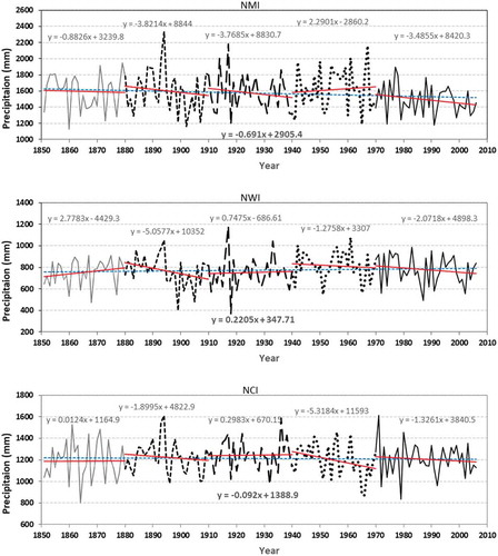
Figure 2. (Continued).

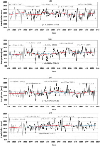
Figure 3. Long-term and short-term linear trends based on monsoon precipitation series of each zone.

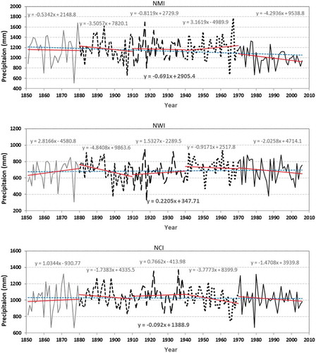
Figure 3. (Continued).

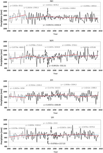
In past studies, drastic changes were found in climatic parameters in the most recent 30-year climate period (1981–2010) (Mirza et al. 1998, Kahya and Kalaycı 2004, Gosain et al. 2006, Pandey et al. 2017). In this study, negative trend lines were found in the last climatic period (C5) (1971–2006) for zones NMI, NWI, NCI and SPI. However, positive trend lines were found for zones NEI, WPI and EPI for the C5 period based on annual time series (Fig. 2).

Positive linear trends were found over zones NWI, WPI, EPI and SPI, with the other zones (NMI, NCI and NEI) indicating a negative trend for long-term monsoon series (Fig. 3). For the C5 time period, most of the zones (NMI, NWI, NCI, NEI and SPI) indicate a negative trend line for monsoon series.

4.3 Sequential trend analysis of annual and monsoon series

In order to examine the trend, the sequential MK test was applied on the annual and monsoon precipitation series. In Figure 4, the Z value is shown for annual and monsoon based data (spring, summer, monsoon and autumn) for each zone. Trends were examined at the 0.05 (5%) significance level of a two-tailed test. The standard value of Z at a significance level of 0.05 (5%) is ±1.96; in Figure 4, the straight dotted lines indicate the upper bound (Z = +1.96) and lower bound (Z = −1.96). The SQMK Z values greater than the upper bound indicate a positive trend, whereas Z values beyond the lower bound indicate a negative trend. In Table 5 it may be seen that for the monsoon season there is a positive trend in zones NMI (Z = +2.93) and NEI (Z = +1.53), whereas a negative trend is found for zones WPI (Z = −2.23) and SPI (Z = −1.11). For the annual series, zone NMI shows a positive trend (Z = +1.91), whereas in zones EPI (Z = −1.64), SPI (Z = −1.70) and WPI (Z = −2.71), a negative trend was found. The sequential MK test was applied separately to the decomposed series (detail and approximation components) of annual, monsoon and monthly precipitation series.

Table 2. Maximum level of decomposition proposed for monthly and yearly series (1851–2006).

Series	Mother wavelet
	db5	db6	db7	db8	db9	db10
Monthly	7	7	7	6	6	6
Yearly	4	3	3	3	3	3
Seasonal	4	3	3	3	3	3

Table 3. Mean relative error (MRE) and Z value relative error (E_r) at different decomposition levels for All India (AI) monthly series (1851–2006). Bold values indicate the minimum values corresponding to “db”.

Wavelet	db5	db6	db7	db8	db9	db10
L	7	7	7	6	6	6
MRE	4.1264	4.1394	4.1401	4.1379	4.1323	4.1336
Er	14.942	14.392	11.811	11.935	13.358	10.262

Table 4. Mean relative error (MRE) and Z value relative error (E_r) at different decomposition levels for AI annual series (1851–2006). Bold values indicate the minimum values corresponding to “db”.

Wavelet	db5	db6	db7	db8	db9	db10
L	4	3	3	3	3	3
MRE	0.1138	0.1095	0.1101	0.1097	0.1094	0.1100
Er	2.154	1.525	1.727	1.584	1.777	1.605

Table 5. MK test (Z value) for original precipitation series (O) and combinations of detailed and approximation series, with coefficient of determination (R²) and NS values. *indicates trend at the 5% significance level, bold indicates the most effective periodic component.

Region	Annual							Monsoon
	O	d1	d2	d3	d1+a3	d2+a3	d3+a3	O	d1	d2	d3	d1+a3	d2+a3	d3+a3
NMI	R^2		0.00	0.10	0.00	0.02	0.12	0.17		0.00	0.10	0.00	0.59	0.54	0.54
	NS		−48.11	−48.38	−47.79	−0.82	0.03	0.16		−48.42	−48.45	−47.74	0.59	0.54	0.28
	Z	1.91	0.20	0.03	−0.10	2.68*	2.88*	3.57*	2.94*	0.01	−0.20	−0.04	3.80*	4.00*	4.50*
NWI	R^2		0.30	0.05	0.10	0.67	0.34	0.26		0.30	0.04	0.07	0.69	0.36	0.36
	NS		−33.83	−32.51	−32.41	0.67	0.34	0.26		−32.01	−32.53	−32.41	0.69	0.36	0.24
	Z	−0.82	0.21	−0.14	0.04	−1.03	−1.79	−1.83	−0.51	0.24	0.00	−0.05	−0.49	−1.01	−1.06
NCI	R^2		0.19	0.03	0.08	0.65	0.37	0.21		0.19	0.03	0.05	0.62	0.45	0.45
	NS		−65.54	−64.46	−64.36	0.65	0.37	0.21		−63.94	−64.44	−64.36	0.62	0.45	0.24
	Z	0.28	0.20	0.12	−0.65	0.37	0.86	0.74	0.52	0.11	0.10	−0.29	0.63	0.81	0.81
NEI	R^2		0.09	0.02	0.07	0.62	0.38	0.25		0.03	0.02	0.04	0.60	0.34	0.34
	NS		−142.54	−141.58	−141.77	0.62	0.38	0.25		−141.31	−141.49	−141.77	0.60	0.34	0.31
	Z	0.33	−0.02	−0.66	−0.19	0.40	0.17	0.20	1.53	0.02	−0.43	0.15	2.08*	2.94*	2.36*
WPI	R^2		0.19	0.07	0.07	0.65	0.45	0.33		0.17	0.06	0.05	0.65	0.42	0.42
	NS		−36.37	−35.34	−35.33	0.65	0.45	0.33		−34.96	−35.33	−35.35	0.65	0.42	0.28
	Z	−2.71*	−0.19	0.19	0.12	−3.73*	−4.09*	−4.41*	−2.23*	−0.09	0.13	0.06	−3.17*	−3.76*	−4.29*
EPI	R^2		0.27	0.03	0.07	0.74	0.35	0.26		0.16	0.00	0.03	0.74	0.34	0.34
	NS		−56.08	−54.89	−54.71	0.74	0.35	0.26		−54.48	−54.86	−54.77	0.74	0.34	0.32
	Z	−1.64	−0.07	0.17	0.00	−1.87	−2.41*	−3.29*	−1.33	−0.22	0.17	−0.04	−1.58	−1.96*	−2.42*
SPI	R^2		0.16	0.09	0.06	0.64	0.38	0.31		0.07	0.04	0.02	0.69	0.32	0.32
	NS		−72.83	−71.74	−71.96	0.64	0.38	0.31		−71.63	−71.83	−71.94	0.69	0.32	0.23
	Z	−1.70	−0.13	−0.31	0.03	−2.98*	−3.32*	−4.07*	−1.11	−0.55	−0.23	0.05	−1.50	−2.17*	−2.32*

Figure 4. Annual and monsoon SQMK test (Z value) plots for each zone.

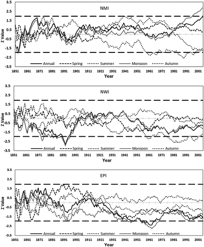
Figure 4. (Continued).

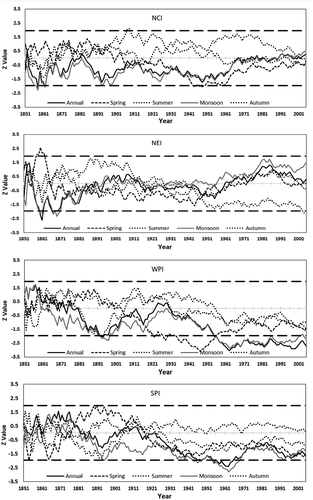
Trend analysis of annual and monsoon time series shows a similar type of trend for most of the zones. Similarity of trend depends on the contribution of average monsoon rainfall to annual rainfall. For example, for zone SPI, the trend deviation for annual and monsoon series is large because the contribution of average monsoon rainfall is around 59.5% of the average annual rainfall. At the same time, the zone having a higher contribution of average monsoon rainfall with respect to average annual rainfall shows a more similar trend, for example NWI (88.8%) and NCI (84.7%).

4.4 Trend analysis using DWT

In this study, the Daubechies (db) wavelet was used because it is the most common smooth mother wavelet for hydro-meteorological study. The relatively large number of data points used in this study were from the monthly, annual and seasonal datasets. Analysis was carried out for the period 1851–2006, on annual and average monsoon data points of 156 years; there were 1872 (12 × 156) data points for the monthly sets. First, the decomposition level was determined to avoid unnecessary levels of data decomposition of these larger datasets (Equation (14)). This level of decomposition is based upon the number of data points and the mother wavelet used de Artigas et al. (2006):

(14)

where v is the number of vanishing moments of a db wavelet, n is the number of data points, and L is the maximum decomposition level. The maximum level of decomposition is shown in Table 2 for monthly, annual and seasonal datasets.

In order to analyse the trend detection, smoother db wavelets (db5–db10) were applied on the monthly and annual datasets. The selection of smoother wavelets was preferred in this study because the trends are supposed to be gradual and represent slowly changing processes.

The criterion used to determine the smooth mother wavelet and the extension mode of db wavelets for the analysis was the mean relative error (MRE) (de Artigas et al. 2006, Nalley et al. 2012, Joshi et al. 2016)). The mean relative error (MRE) was calculated as:

(15)

where is the original data value, and is the approximation of. In the results, it was found that there were no significant differences in values of MRE. The second criterion is the relative error (E_r), proposed by (Nalley et al. 2012, 2013). The lowest value of E_r, based on approximation of the MK test Z value, was examined for each extension mode of the smooth db wavelets. The relative error is calculated as:

(16)

where is the Z value (MK test) of the last approximation for the decomposed level used, and is the MK test Z value of the original data. The results of MRE and E_r calculations are given in Table 3 and Table 4 for monthly and annual values, respectively. In the results, it was found that the db10 wavelet showed the lowest value of MRE and E_r for monthly datasets, whereas the db6 wavelet was found more suitable for annual data.

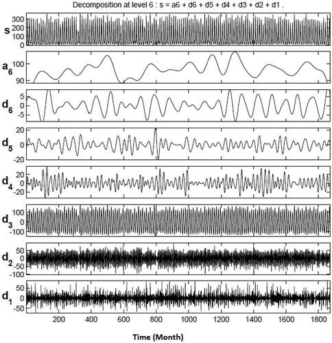
Figures 5 and 6 show the decomposed level for annual and monthly time series using the DWT method. It can be seen in Figures 5 and 6 that more detailed decomposed levels have lower frequencies, which shows the change in periodicity. The approximation components (a3 and a6) show the long-term change in trend.

Figure 5. Decomposition of original annual precipitation series of All India (AI) into three levels (d1–d3) and approximation (a3).

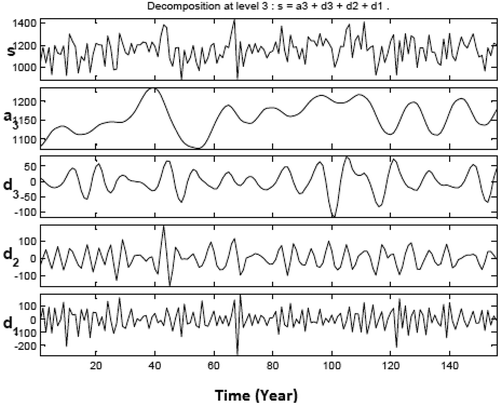
Figure 6. Decomposition of original monthly precipitation series of AI into six levels (d1–d6) and approximation (a6).

4.5 Trend analysis of decomposed annual, monsoon and monthly series

Each annual and seasonal time series was decomposed into three detailed components (d1–d3) and one approximation (a3), and the monthly series was decomposed into six components (d1–d6) and one approximation (a6). Each detailed component represents the 2ⁿ (dyadic translation) fluctuations, where n is the level of detailed components. For annual and monsoon detailed series, d1, d2 and d3 represent the 2-year, 4-year and 8-year periodicity, respectively. The approximate component of the wavelet transform represents the high-scale function of the time series. Moreover, it is the low-frequency component of the time series and is used to find the key points of the time series to lose minimum potential information (He et al. 2016). For this study, a3 is found as the end point for deriving the optimal (maximum/minimum) local points of precipitation time series for India. Therefore, for monthly series, detailed components d1, d2, d3, d4, d5 and d6 represent the 2-, 4-, 8-, 16-, 32- and 64-month periodicity, respectively.

A comparison was carried out between the original series and the combination of decomposed series. The values of evaluation parameters, coefficient of determination (R²) and Nash-Sutcliffe efficiency coefficient (NS), are given in Table 5.

Table 5 indicates that only a few zones showed a significant trend, for example WPI for annual rainfall, and NMI for both annual and monsoon season rainfall. Zone WPI indicates a negative trend for annual and monsoon season, whereas a positive trend was detected for the NMI monsoon season. It is quite interesting to see the significant trend in decomposed components, where the original series did not show a significant trend, e.g. NMI, NEI (monsoon), EPI and SPI zones (Table 5). In general, combinations of detailed and approximation series indicated an increase in MK test Z value as compared to single detailed series (without approximation series) and original series. The results shown in Table 5 imply that the combination of detailed and approximation series mainly contributed to the trend in the original series. However, all the decomposed components of periodicity did not have much influence on the trend of the original series.

While analysing the Z values of the individual detailed series and the combination of detailed and approximation series, it was noticed that individual detailed series did not show the closeness to the original series (excluding zone NCI for the d1 series), although all zones were examined for significant trend, which was found in WPI and NMI (monsoon). However, in all cases, the combination of d1+a3 showed the nearest Z value to the original series (annual and monsoon precipitation time series).

Hence, it is clear that the approximation component carries the trend components and affects the trend in the original series, which is similar to the results mentioned by Nalley et al. (2012) in analysing the Quebec and Ontario (Canada) region. For example, for the NMI zone (Z = +1.91) the detailed series (d1) Z value is 0.20, whereas for the combination series (d1+a3) it is 2.68, which also shows a significant trend.

Nalley et al. (2012) proposed a two-step method to identify the most effective periodic components in contributing to trend in the original series. In the first step, the SQMK approach is applied to check the progressive trend line of each individual detailed series and combinations of detailed and approximation series with respect to original time series. Thus, the detailed series, or combination of detailed and approximation series, that follow the same trend as the original data could be identified. In the second step, the MK test Z values of the detailed series and combinations of detailed and approximation series are compared with the Z value of the original time series, and the closet values identified. The component(s) that satisfy these two tests are considered as the most dominant components that affect the trend.

In this study, the combination of detailed components and combinations with approximations were evaluated to identify the most influential component of the trend (Nalley et al. 2012). While analysing the Z values of the different combinations, it was noticed that combination of two or more detailed components with the approximation component significantly increased the Z value of the series. However, these combinations do not play a crucial role in the decision making, as the Z value is far away from the Z value of the original series, and at the same time the SQMK graph does not match. Hence, we considered a combination of single detailed components with approximation series for comparison of Z values and SQMK graph (Figs 7–9, Tables 5 and 6).

Table 6. MK test (Z value) for monthly series, detail components (D1–D6), approximation (A3) and combinations of detail and approximation. * indicates trend at the 5% significance level, bold indicates the most effective periodic component.

	Monthly series (1851–2006)
	NCI	NWI	EPI	NMI	SPI	WPI	NEI
Original	−0.70	−1.22	−0.77	−0.86	−1.37	−1.35	0.00
D1	0.30	−0.28	−0.04	0.33	−0.16	0.11	−0.12
D2	0.13	0.09	0.01	0.46	0.05	0.12	−0.02
D3	−0.22	−0.03	0.01	−0.42	−0.11	0.10	−0.16
D4	0.04	0.34	0.49	0.42	0.11	0.21	0.28
D5	0.07	0.13	0.35	−0.52	0.42	0.23	−0.17
D6	−0.16	−0.21	0.39	0.70	1.20	0.36	−0.55
A6	3.65*	−5.27*	−11.72*	12.50*	−20.85*	−16.73*	2.32*
D1+A6	0.88	−1.40	−2.56*	2.68*	−3.40*	−3.72*	0.95
D2+A6	0.44	−0.59	−2.34*	1.76	−2.71*	−2.77*	0.61
D3+A6	0.03	−0.50	−0.94	0.70	−1.65	−1.39	0.12
D4+A6	1.11	−2.62*	−5.53*	5.96*	−7.33*	−7.70*	2.02*
D5+A6	0.90	−2.93*	−7.75*	7.52*	−9.98*	−12.12*	0.94
D6+A6	2.75*	−5.00*	−9.52*	10.41*	−11.75*	−14.42*	0.64

Figure 7. Changes in trend in time for annual original series and combinations of detailed and approximation series.

Figure 8. Changes in trend in time for monsoon original series and combinations of detailed and approximation series.

Figure 9. Changes in trend in time for monthly original series and combinations of detailed and approximation series.

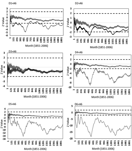
In this study, the most periodic component was identified as d1 which contributed a 2-year periodicity trend (with addition to the approximation series) for annual and monsoon series over the study area (Table 5, Figs 7 and 8). This indicates that d2 (4-year periodicity) and d3 (8-year periodicity) did not contribute much in the trend of the annual and monsoon season rainfall in the study area.

Table 6 shows zone-wise MK test Z values for monthly series from 1850 to 2006 (1872 data points) for the study area. There was no significant trend in the study area for the original monthly time series. In general, the most dominating periodicity was d3 (with approximation series), except in zones NWI (d1) and NEI (d2). Hence, the 8-month periodicity was the most influential parameter for estimating rainfall trends in the study area (Fig. 9). The results also emphasize the usefulness of monthly trend analysis along with decomposed components using wavelet techniques, as in the present study. Monthly analysis seems important because the periodicity was found to be less than for yearly data.

4.6 Visualization and thresholding of precipitation extreme events

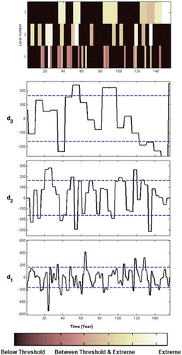
In order to analyse the contributing events for extreme events, the method of wavelet analysis is very valuable to decompose the original time series into different frequencies, retaining information in the time domain (Labat 2005, Chou 2011, Nalley et al. 2013). Figure 10 presents an example of normalized annual precipitation time series of zone WPI; in the bottom panel the horizontal (blue, red and green) lines represent the three selected thresholds for both positive and negative positions. These thresholds were selected based on the standard deviation (S in Figs. 10 and 11) of the original precipitation series. Figure 10 clearly shows that the number of exceedence events decreases as the threshold increases. Figure 11 shows a visualization of the extreme value of monsoon precipitation at fixed threshold values over the WPI zone. In Figures 10 and 11, black represents non-exceedence properties of the series. The approach taken here was inspired by the work of Keylock (2007), but applies to time series of precipitation data. The method could be generalized to gain frequency information from the precipitation time series. An inspection of Figure 10 clearly shows that the exceedence of 1.5S at t = 20 (negative fluctuation) is a different type of event from that at t = 65 (positive fluctuation). The different shades indicate the different frequency fluctuations. Keylock (2007) stated, “The former arises due to relatively small high frequency fluctuations superimposed on a large, low frequency positive departure from the mean. The latter is a sudden and dramatic excursion from the mean that is not superimposed on an obvious larger scale fluctuation”. Therefore, it helps to visualize this information in a clear manner so that the scales of events that actively contribute to an extreme event can be determined.

Figure 10. Visualization of detailed component (d1) extreme values of annual precipitation at different threshold values of standard deviation (S) over the WPI zone of India. Red, green and blue lines indicate the threshold values at, respectively, 0.5, 1.0 and 1.5 times the standard deviation of the observed series.

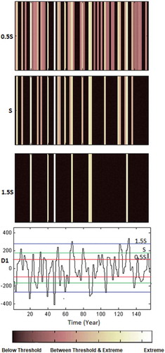
Figure 11. Visualization of extreme values of monsoon precipitation at fixed threshold values over the WPI zone of India. Dashed (blue) lines in d1, d2 and d3 indicate the threshold values (standard deviation of the original series).

5 Conclusions

In this study, trend detection has been carried out for long-term precipitation data over India, applying regression analysis, the MK test and a combination of DWT and sequential MK tests. Regression analysis was carried out on the basis of the classical climate period of 30 years. The results of this study imply that the mean values of precipitation are decreasing in most of the study area in the last 30-year period. It was found that there are both positive and negative trends existing in each zone for the monsoon datasets. Annual and monsoon precipitation data show a negative trend; however, zones NMI and NEI show a positive trend for annual and monsoon datasets. The most suitable mother wavelet was selected using the criteria of MRE and the criterion relative error (E_r) proposed by Nalley et al. (2012). Applying this criterion, the DWT Daubechies wavelets db6 and db10 were selected for annual and monthly datasets, respectively. The decomposed level was determined using the extension border of DWT and the length of the datasets. The comparisons were carried out between the original series and decomposed series in terms of R² and NS values. The Z statistic was evaluated for trend analysis of the decomposed periodic components and the original annual and monsoon series. Application of DWT on annual series implied 2-, 4- and 8-year fluctuations in the NMI zone, indicating a positive trend in rainfall, whereas zones WPI, SPI and WPI (with 2- and 4-year fluctuations) experienced a negative trend at the same periodicities, at the 0.05 (5%) significance level. In the monsoon series, a positive trend was found over NMI and NEI decomposed series at 2-, 4- and 8-year periodicity, whereas WPI, EPI and SPI indicated a negative trend at the same periodicity. Considering India as whole (AI), a negative trend was found in all zones except NMI and NEI. Therefore, visualization of extreme events was examined at different threshold limits. The same intensity of positive and negative fluctuations indicated the same colour spectrum, which is one of the limitations of the visualization study and may form the subject of future work in this area.

Acknowledgements

The authors wish to thank IIT Roorkee for providing the needful space and resources during the study.

Disclosure statement

No potential conflict of interest was reported by the authors.

Additional information

Funding

This work was financially supported by the Ministry of Human Resources and Development, New Delhi, and the Department of Science and Technology, New Delhi.

References

- Adarsh, S. and Janga Reddy, M., 2015. Trend analysis of rainfall in four meteorological subdivisions of southern India using nonparametric methods and discrete wavelet transforms. International Journal of Climatology, 35 (6), 1107–1124. doi:10.1002/joc.2015.35.issue-6
- Agarwal, A., et al., 2005. ANN-based sediment yield models for Vamsadhara river basin (India). Water SA, 31 (1), 85–100. doi:10.4314/wsa.v31i1.5125
- Ahmad, S. and Simonovic, S.P., 2005. An artificial neural network model for generating hydrograph from hydro-meteorological parameters. Journal of Hydrology, 315 (1), 236–251. doi:10.1016/j.jhydrol.2005.03.032
- Anandhi, A., et al., 2013. Long-term spatial and temporal trends in frost indices in Kansas, USA. Climatic Change, 120 (1), 169–181. doi:10.1007/s10584-013-0794-4
- Barkhordarian, A., Bhend, J., and von Storch, H., 2012. Consistency of observed near surface temperature trends with climate change projections over the Mediterranean region. Climate Dynamics, 38 (9–10), 1695–1702. doi:10.1007/s00382-011-1060-y
- Chakraborty, A. and Okaya, D., 1995. Frequency-time decomposition of seismic data using wavelet-based methods. Geophysics, 60 (6), 1906–1916. doi:10.1190/1.1443922
- Chou, C.-M., 2011. A threshold based wavelet denoising method for hydrological data modelling. Water Resources Management, 25 (7), 1809–1830. doi:10.1007/s11269-011-9776-3
- Clementsa, M.P., Norman, P.H.F., and Swansonc, R., 2004. Forecasting economic and financial time-series with non-linear models. International Journal of Forecasting, 20, 169–183. doi:10.1016/j.ijforecast.2003.10.004
- de Artigas, M.Z., Elias, A.G., and de Campra, P.F., 2006. Discrete wavelet analysis to assess long-term trends in geomagnetic activity. Physics and Chemistry of the Earth, Parts A/B/C, 31 (1–3), 77–80. doi:10.1016/j.pce.2005.03.009
- Dibike, Y.B. and Coulibaly, P., 2005. Hydrologic impact of climate change in the Saguenay watershed: comparison of downscaling methods and hydrologic models. Journal of Hydrology, 307 (1–4), 145–163. doi:10.1016/j.jhydrol.2004.10.012
- Duhan, D., et al., 2013. Spatial and temporal variability in maximum, minimum and mean air temperatures at Madhya Pradesh in central India. Comptes Rendus Geoscience, 345 (1), 3–21. doi:10.1016/j.crte.2012.10.016
- Fowler, H.J., Blenkinsop, S., and Tebaldi, C., 2007. Linking climate change modelling to impacts studies: recent advances in downscaling techniques for hydrological modelling. International Journal of Climatology, 27 (12), 1547–1578. doi:10.1002/(ISSN)1097-0088
- Gocic, M. and Trajkovic, S., 2013. Analysis of changes in meteorological variables using Mann-Kendall and Sen’s slope estimator statistical tests in Serbia. Global and Planetary Change, 100, 172–182. doi:10.1016/j.gloplacha.2012.10.014
- Gosain, A., Rao, S., and Basuray, D., 2006. Climate change impact assessment on hydrology of Indian river basins. Current Science, 90 (3), 346–353.
- Goswami, B.N., et al., 2006. Increasing trend of extreme rain events over India in a warming environment. Science, 314 (5804), 1442–1445. doi:10.1126/science.1132027
- Goyal, M., 2014. Statistical analysis of long term trends of rainfall during 1901–2002 at Assam, India. Water Resources Management, 28 (6), 1501–1515. doi:10.1007/s11269-014-0529-y
- Hamlet, A.F., et al., 2007. Twentieth-century trends in runoff, evapotranspiration, and soil moisture in the Western United States. Journal of Climate, 20 (8), 1468–1486. doi:10.1175/JCLI4051.1
- He, X., Shao, C., and Xiong, Y., 2016. A non-parametric symbolic approximate representation for long time series. Pattern Analysis and Applications, 19 (1), 111–127. doi:10.1007/s10044-014-0395-5
- Holman, I.P., 2005. Climate change impacts on groundwater recharge- uncertainty, shortcomings, and the way forward? Hydrogeology Journal, 14 (5), 637–647. doi:10.1007/s10040-005-0467-0
- Ivanov, P.C., et al., 1996. Scaling behaviour of heartbeat intervals obtained by wavelet-based time-series analysis. Nature, 383 (6598), 323–327. doi:10.1038/383323a0
- Ivanov, P.C., et al., 1999. Multifractality in human heartbeat dynamics. Nature, 399 (6735), 461–465. doi:10.1038/20924
- Jain, S.K., Kumar, V., and Saharia, M., 2013. Analysis of rainfall and temperature trends in northeast India. International Journal of Climatology, 33 (4), 968–978. doi:10.1002/joc.v33.4
- Joos, F., et al., 2001. Global warming feedbacks on terrestrial carbon uptake under the Intergovernmental Panel on Climate Change (IPCC) emission scenarios. Global Biogeochemical Cycles, 15 (4), 891–907. doi:10.1029/2000GB001375
- Joshi, N., et al., 2016. Analysis of trends and dominant periodicities in drought variables in India: A wavelet transform based approach. Atmospheric Research, 182, 200–220. doi:10.1016/j.atmosres.2016.07.030
- Kahya, E. and Kalaycı, S., 2004. Trend analysis of streamflow in Turkey. Journal of Hydrology, 289 (1–4), 128–144. doi:10.1016/j.jhydrol.2003.11.006
- Kendall, M.G., 1975. Rank correlation methods. London: Charles Griffin.
- Keylock, C.J., 2007. The visualization of turbulence data using a wavelet-based method. Earth Surface Processes and Landforms, 32 (4), 637–647. doi:10.1002/(ISSN)1096-9837
- Kisi, O. and Cimen, M., 2012. Precipitation forecasting by using wavelet-support vector machine conjunction model. Engineering Applications of Artificial Intelligence, 25 (4), 783–792. doi:10.1016/j.engappai.2011.11.003
- Klein Tank, A. and Können, G., 2003. Trends in indices of daily temperature and precipitation extremes in Europe, 1946–99. Journal of Climate, 16 (22), 3665–3680. doi:10.1175/1520-0442(2003)016<3665:TIIODT>2.0.CO;2
- Labat, D., 2005. “Recent advances in wavelet analyses: part 1. A review of concepts. Journal of Hydrology, 314 (1–4), 275–288. doi:10.1016/j.jhydrol.2005.04.003
- Labat, D., Ronchail, J., and Guyot, J.L., 2005. Recent advances in wavelet analyses: part 2—amazon, Parana, Orinoco and Congo discharges time scale variability. Journal of Hydrology, 314 (1–4), 289–311. doi:10.1016/j.jhydrol.2005.04.004
- Lettenmaier, D.P., Wood, E.F., and Wallis, J.R., 1994. Hydro-climatological trends in the continental United States, 1948–88. Journal of Climate, 7 (4), 586–607. doi:10.1175/1520-0442(1994)007<0586:HCTITC>2.0.CO;2
- Li, L., et al., 2014. Validation of a new meteorological forcing data in analysis of spatial and temporal variability of precipitation in India. Stochastic Environmental Research and Risk Assessment, 28 (2), 239–252. doi:10.1007/s00477-013-0745-7
- Lu, M., 1997. Trends in surface air temperature data over Turkey. International Journal of Climatology, 17, 511–520. doi:10.1002/(SICI)1097-0088(199704)17:5<511::AID-JOC130>3.0.CO;2-0
- Mann, H.B., 1945. Nonparametric tests against trend. Econometrica: Journal of the Econometric Society, 13 (3), 245–259.
- Meehl, G.A., et al., 2007. Global climate projections. Climate Change, 283, 747–845.
- Meenu, R., Rehana, S., and Mujumdar, P., 2013. Assessment of hydrologic impacts of climate change in Tunga–Bhadra river basin, India with HEC‐HMS and SDSM. Hydrological Processes, 27 (11), 1572–1589. doi:10.1002/hyp.v27.11
- Mehrotra, R., et al., 2013. Assessing future rainfall projections using multiple GCMs and a multi-site stochastic downscaling model. Journal of Hydrology, 488, 84–100. doi:10.1016/j.jhydrol.2013.02.046
- Mekis, É. and Vincent, L.A., 2011. An overview of the second generation adjusted daily precipitation dataset for trend analysis in Canada. Atmosphere-Ocean, 49 (2), 163–177. doi:10.1080/07055900.2011.583910
- Mirza, M., et al., 1998. Trends and persistence in precipitation in the Ganges, Brahmaputra and Meghna river basins. Hydrological Sciences Journal, 43 (6), 845–858. doi:10.1080/02626669809492182
- Murumkar, A.R. and Arya, D.S., 2014. Trend and periodicity analysis in rainfall pattern of Nira Basin, Central India. American Journal of Climate Change, 3 (01), 60. doi:10.4236/ajcc.2014.31006
- Nalley, D., et al., 2013. Trend detection in surface air temperature in Ontario and Quebec, Canada during 1967–2006 using the discrete wavelet transform. Atmospheric Research, 132, 375–398. doi:10.1016/j.atmosres.2013.06.011
- Nalley, D., Adamowski, J., and Khalil, B., 2012. Using discrete wavelet transforms to analyze trends in streamflow and precipitation in Quebec and Ontario (1954–2008). Journal of Hydrology, 475, 204–228. doi:10.1016/j.jhydrol.2012.09.049
- Nikhil Raj, P.P. and Azeez, P.A., 2012. Trend analysis of rainfall in Bharathapuzha River basin, Kerala, India. International Journal of Climatology, 32 (4), 533–539. doi:10.1002/joc.v32.4
- Pachauri, R.K., et al., 2014. “Climate change 2014: synthesis report. Contribution of Working Groups I, II and III to the Fifth Assessment Report of the Intergovernmental Panel on Climate Change.”
- Pandey, B.K., Gosain, A.K., Paul, G., & Khare, D., 2017. Climate change impact assessment on hydrology of a small watershed using semi-distributed model. Applied Water Science, 7 (4), 2029–2041.
- Partal, T. and Küçük, M., 2006. Long-term trend analysis using discrete wavelet components of annual precipitations measurements in Marmara region (Turkey). Physics and Chemistry of the Earth, Parts A/B/C, 31 (18), 1189–1200. doi:10.1016/j.pce.2006.04.043
- Parth Sarthi, P., Ghosh, S., and Kumar, P., 2015. Possible future projection of Indian Summer Monsoon Rainfall (ISMR) with the evaluation of model performance in Coupled Model Inter-comparison Project Phase 5 (CMIP5). Global and Planetary Change, 129, 92–106. doi:10.1016/j.gloplacha.2015.03.005
- Rahmani, V., Hutchinson, S.L., Harrington Jr, J.A., Hutchinson, J.M., & Anandhi, A., 2015. Analysis of temporal and spatial distribution and change-points for annual precipitation in Kansas, USA. International Journal of Climatology, 35 (13), 3879–3887.
- Randall, D.A., et al., 2007. Climate models and their evaluation. Climate Change 2007: the physical science basis. Contribution of Working Group I to the Fourth Assessment Report of the IPCC (FAR), Cambridge: Cambridge University Press, 589–662.
- Reeves, J., et al., 2007. A review and comparison of changepoint detection techniques for climate data. Journal of Applied Meteorology and Climatology, 46 (6), 900–915. doi:10.1175/JAM2493.1
- Ribbe, L., et al., 2017. Integrated river basin management in the Vu Gia Thu Bon Basin. In: A. Nauditt and L. Ribbe, eds. Land use and climate change interactions in central vietnam. Singapore: Springer, 153–170.
- Sang, Y.-F., et al., 2009. Entropy-based wavelet de-noising method for time series analysis. Entropy, 11 (4), 1123–1147. doi:10.3390/e11041123
- Sethi, R., et al., 2015. Performance evaluation and hydrological trend detection of a reservoir under climate change condition. Modeling Earth Systems and Environment, 1 (4), 1–10. doi:10.1007/s40808-015-0035-0
- Sinha, S., et al., 2005. Spectral decomposition of seismic data with continuous-wavelet transform. Geophysics, 70 (6), P19–P25. doi:10.1190/1.2127113
- Smith, L.C., Turcotte, D.L., and Isacks, B.L., 1998. Stream flow characterization and feature detection using a discrete wavelet transform. Hydrological Processes, 12 (2), 233–249. doi:10.1002/(ISSN)1099-1085
- Sonali, P. and Kumar, D.N., 2013. Review of trend detection methods and their application to detect temperature changes in India. Journal of Hydrology, 476, 212–227. doi:10.1016/j.jhydrol.2012.10.034
- Sontakke, N.A., Singh, N., and Singh, H.N., 2008. Instrumental period rainfall series of the Indian region (AD 1813—2005): revised reconstruction, update and analysis. The Holocene, 18 (7), 1055–1066. doi:10.1177/0959683608095576
- Tarhule, A., et al., 2015. Exploring temporal hydroclimatic variability in the Niger Basin (1901–2006) using observed and gridded data. International Journal of Climatology, 35 (4), 520–539. doi:10.1002/joc.2015.35.issue-4
- Vittal, H., Karmakar, S., and Ghosh, S., 2013. Diametric changes in trends and patterns of extreme rainfall over India from pre-1950 to post-1950. Geophysical Research Letters, 40 (12), 3253–3258. doi:10.1002/grl.50631
- Wang, W. and Ding, J., 2003. Wavelet network model and its application to the prediction of hydrology. Nature and Science, 1 (1), 67–71.
- Xu, J., et al., 2009. Wavelet analysis and nonparametric test for climate change in Tarim River Basin of Xinjiang during 1959–2006. Chinese Geographical Science, 19 (4), 306–313. doi:10.1007/s11769-009-0306-7
- Zaveri, E., et al., 2016. Invisible water, visible impact: groundwater use and Indian agriculture under climate change. Environmental Research Letters, 11 (8), 084005. doi:10.1088/1748-9326/11/8/084005