Probabilistic and ensemble simulation approaches for input uncertainty quantification of artificial neural network hydrological models

ABSTRACT

Artificial neural network (ANN) has been demonstrated to be a promising modelling tool for the improved prediction/forecasting of hydrological variables. However, the quantification of uncertainty in ANN is a major issue, as high uncertainty would hinder the reliable application of these models. While several sources have been ascribed, the quantification of input uncertainty in ANN has received little attention. The reason is that each measured input quantity is likely to vary uniquely, which prevents quantification of a reliable prediction uncertainty. In this paper, an optimization method, which integrates probabilistic and ensemble simulation approaches, is proposed for the quantification of input uncertainty of ANN models. The proposed approach is demonstrated through rainfall-runoff modelling for the Leaf River watershed, USA.  The results suggest that ignoring explicit quantification of input uncertainty leads to under/over estimation of model prediction uncertainty. It also facilitates identification of appropriate model parameters for better characterizing the hydrological processes.

KEYWORDS:

• artificial neural networks
• ensemble simulation
• input uncertainty
• prediction uncertainty
• rainfall–runoff modelling

Editor R. Woods Associate editor F.-J. Chang

Introduction

The choice of a hydrological model, in general, is based on the complexity of the hydrological processes to be considered in the modelling exercise. To date, a variety of hydrological models have been developed, which are being employed mainly for the effective planning, management and operation of water resource projects. In most situations, the objective of the modelling is to adjust or calibrate the model parameters for capturing the dynamics of the hydrological processes at either the entire catchment scale or sub-catchment scale to obtain an arbitrarily accurate model prediction (Vrugt et al. 2008). Consequently, several optimization techniques and procedures have been developed and/or employed to search for the optimal set of parameters in hydrological models (Kavetski et al. 2006, Tolson and Shoemaker 2007). However, the confidence of such models and calibrated model parameters is limited, due to the presence of uncertainty. Therefore, besides accurate model prediction, evaluating uncertainty in hydrological models, which is another important metric that needs to be considered, has become crucial.

While several components introduce uncertainty in the hydrological process, the inherent variability that exists in the input, parameter and model structure is considered to be a major source of model prediction uncertainty. It has been reported that explicit integration and quantification of these sources would enhance overall hydrological forecasting (Zhang et al. 2011a). However, considering contributions from each source and their mutual interaction while estimating the total prediction uncertainty is computationally a challenging task (Parasuraman and Elshorbagy 2008). For instance, accounting structure uncertainty would lead to a change in the number of model parameters. As a result, one could expect an increase in degrees of freedom associated with model parameters. Similarly, including the input error in the model calibration requires valid assumptions and additional model parameters. Further, it is impossible to determine the true value of input, which is unknown. Hence, most of the previous studies have considered only the parameter uncertainty (Ebtehaj et al. 2010) in the modelling. In such analysis, only a portion of the uncertainty is quantified out of total prediction uncertainty while neglecting other sources of uncertainty. Therefore, it is important to develop modelling procedures that quantify each source of uncertainty, either separately or together, for realistic model prediction. Overall, it would provide insightful results, which could be used for better understanding and characterizing catchment responses.

It has been emphasized that model inputs produce considerable uncertainty, which significantly affects the model prediction (Kavetski et al. 2006, Vrugt et al. 2008, Patil and Deng 2012), besides model parameter (Li et al. 2015) and structure uncertainty (Zhang et al. 2011b). In recent decades, significant research studies have focused on developing methodology for the quantification of input uncertainty along with other sources of uncertainty in hydrological models. These include Bayesian total error analysis (BATEA), Kavetski et al. 2006), differential evolutionary adaptive metropolis (DREAM, Vrugt et al. 2003) and multi-model target distribution (Vrugt et al. 2009). The methods reported in the above studies have been demonstrated mostly through conceptual hydrological models, hence similar methods can be extended to other modelling approaches, such as data-driven models.

Over the past two decades, the accurate prediction of ANN models has gained significant interest among researchers for modelling various hydrological/hydrogeological processes. The ANN model can be developed with limited available information, in order to derive suitable relationships among the modelled variables, whereas the physics-based models require detailed information on the catchment. Numerous research studies have reported the usefulness of ANN in hydrological modelling, such as evapotranspiration modelling (Kumar et al. 2002), infiltration (Nestor 2006), flood forecasting (Chang et al. 2007), flood frequency analysis (He et al. 2015) and so on. Despite improved estimates of modelled variables from the point prediction of ANN, the practical application of these models is limited due to the uncertainty. Hence, there is a growing interest in developing methods to quantify the uncertainty in ANN models (Srivastav et al. 2007, Kasiviswanathan et al. 2013, Tiwari et al. 2013). While a majority of the previous studies have analysed the influence of parameter and structure uncertainty (Zhang et al. 2009), the main focus of the present study is to quantify the input uncertainty of ANN models. In this paper, a probabilistic and ensemble simulation technique combined with a multi-objective optimization method is proposed. In order to demonstrate the influence of input uncertainty on the model prediction uncertainty, two different simulation cases are conducted while estimating model parameters: Case I assumes no input error, and Case II includes input error. The next section describes the proposed methodology. Then the results are analysed and discussed in the succeeding sections. Finally, the summary and conclusions drawn from the study along with scope for further research are presented.

Methodology

The method begins with the conventional approaches used for identifying the inputs and the ANN model architecture. A combination of probabilistic and ensemble simulation-based optimization approaches is proposed to quantify the input uncertainty of ANN in terms of model prediction uncertainty. This is conducted in a two-stage optimization, wherein Stage 1 estimates the input uncertainty, and the prediction uncertainty is quantified in Stage 2.

Identification of model input and ANN architecture

Ignoring the important input and/or including redundant inputs is not advisable, as both would reduce the capability of ANN model prediction. Therefore, model input identification is one of the important steps in ANN modelling. While several methods, ranging from sophisticated optimization algorithms to simple linear correlation, are available, this study used a commonly employed statistical approach to identify the appropriate input variables (Sudheer et al. 2002). The method was based on the heuristic that the potential influencing variables corresponding to different time lags can be identified through statistical analysis of the data series that uses cross-, auto- and partial autocorrelations between the variables in question. It should be noted that the relationships among input variables may be highly non-linear; under this condition the assumption of linear dependency might not be appropriate. Nonetheless, the determination of inputs using a statistical approach is very popular in ANN modelling and it has been reported in a majority of the studies in hydrological modelling (Maier et al. 2010).

This study focused on ANNs in their most common form, the multilayer perceptron (MLP), but other ANN-based approaches exist; for example, radial basis function (RBF) networks and recurrent neural networks (Kumar et al. 2005). Several studies have been reported that compared the performance of MLP with RBF and other variants of ANN, and suggested that MLP outperforms the others in hydrological applications (Maier et al. 2010). This study used MLPANN architecture, which has three layers including an input layer, one or more hidden layer, and an output layer. Each layer consists of a number of nodes, in which the weights and biases (i.e. model parameters) are the numerical values introduced into the network between different nodes in the form of connections. The choice of the number of hidden layers is based on the complexity of the process to be modelled. However, including multiple hidden layers might result in overfitting of the data used for developing the model. Thus, a single hidden layer is most prevalent (Maier et al. 2010). The number of input and output nodes is dependent on the modeller, whereas the number of hidden nodes is fixed based on the model performance; accordingly, the ANN model architecture is decided. Different approaches have been reported in the literature (Maier et al. 2010), including global, stepwise and trial and error. Despite the superiority of the global and stepwise approaches, the trial-and-error approach has often been reported due to its simplicity and lower computational requirement (Nayak et al. 2005); thus it was used to optimize the ANN in this paper. The trial-and-error approach starts with two hidden neurons, and the number of hidden neurons is increased by 1 in each trial. The final architecture of the ANN model is identified by repeated iterations, which continue until there is no further significant improvement in the model performance.

Optimization stage 1: input uncertainty quantification

The error in the input may exist in a particular variable or the complete set of variables used for developing the model. In this paper, the error in the rainfall was considered as a major source of input uncertainty, which propagates to the model prediction. It has been reported that analysing input uncertainty should yield meaningful values of model parameters, which, in general, has significant implications for testing hydrological theory, diagnosing structural errors in models, and appropriately benchmarking rainfall measurement devices (Vrugt et al. 2008). In principle, each rainfall value is associated with an independent error. The error can be attributed to various sources, such as interpolation error, measurement error and sampling error. Therefore, the input error in each measured value must be estimated independently when estimating the model parameters in the model calibration. However, the major difficulty in such an approach is the dimensionality in the calibration procedure, which grows multifold. In addition to that, the predictive capability of model might deteriorate gradually due to overparameterization (Vrugt et al. 2008). Therefore, it is necessary to develop efficient methods that quantify input uncertainty in the model by accomplishing the condition of a parsimonious model.

The traditional calibration of the ANN model (Equation (1)) assumes that there is no input error, as the measured values are considered to be true values (i.e.), where represent the measured and true rainfall values, respectively. Note that the rainfall only is shown in Equation (1), to demonstrate the methodology, and other inputs were also included in the model development. Details about including inputs such as rainfall and evapotranspiration are presented in the “Results and discussion” section.

(1)

where y_t represents the target variable of the tth pattern; i, j and k are the indices representing input, hidden and output layers, respectively; p is the total number of inputs used for developing the model; M is the dimension of ANN architecture in terms of number of hidden neurons; and β_j and β_k denote the bias of hidden and output nodes, respectively. Similarly, w_ij denotes the weights connecting input to hidden nodes and w_jk denotes weights connecting hidden to output nodes.

The assumption in Equation (1) is valid only when the measured rainfall values contain no error; in other words, the values are not disturbed by aforementioned factors (i.e. instrument error, human error, etc.). However, such a condition is ideal and may not exist, while the process of measuring rainfall has high variability in an uncertain environment. In addition, the deviation of the measured value from its true value is unknown, which makes it difficult to characterize the input error. Therefore, the measured values need to be corrected/adjusted to closely follow the true values. In this paper, a modelling procedure is developed that can diagnose the input error in the model calibration. This can be achieved through forcing various realizations of error in the measured rainfall, referred to as the rainfall multiplier (). Based on this approach, the forcing errors (i.e. perturbations) were introduced in the measured input values. The forcing error is generally sampled from probability distribution functions (Vrugt et al. 2008, Yen et al. 2015). The forcing error herein was assumed to follow a log-normal distribution as the multiplier needs to be a positive fraction. The normal distribution may not be an appropriate choice as it requires additional computation to change the domains of values into a positive fraction. The initial values of the parameters of the log-normal distribution, i.e. mean (µ) and standard deviation (σ) of the probability density function (pdf), were assumed based on the maximum amount of error that the measured rainfall might have; these values were then estimated through the model calibration. As mentioned above, the error is identical and independent, hence the value of was sampled from the log-normal probability distribution function, with calibrated µ and σ, for each rainfall value. Ideally, the input error should have a mean value of zero, and the corresponding mean value in the log-normal domain (equal to 1.0) was considered in this study. The value of σ was obtained through calibration along with the other ANN parameters. The root mean square error (RMSE) was used as the objective function in the genetic algorithm (GA) based optimization approach (NSGA-II; Deb et al. 2002) to simultaneously calibrate the neural network weights and the parameter σ of the log-normal distribution. The lower and upper bounds of σ were fixed as 0.0 and 0.25, respectively, through trial and error. The lower and upper bounds of the ANN parameters were fixed at −10 and +10, as suggested by Dhanesh and Sudheer (2011). The values of GA parameters, such as number of generation, population, probability of cross-over and probability of mutation, were identified through sensitivity analysis and were fixed at 1000, 100, 0.6 and 0.001, respectively.

The sampled value of the multiplier was then used to adjust the measured rainfall into error forced rainfall () independently. Subsequently, the ANN model presented in Equation (1) was modified to the following form, which includes the rainfall multiplier:

(2)

As mentioned previously, a two-stage optimization procedure, as demonstrated in Kasiviswanathan et al. (2013) and Ye et al. (2014), was applied to account for the input uncertainty, and to quantify the model prediction uncertainty. In the first stage of optimization, the plausible input uncertainty was assessed while calibrating the suitable parameter sets of the ANN model. The flowchart (Fig. 1) illustrates the parameter optimization (Stage 1), which incorporates the rainfall multiplier. During this stage of optimization, the decision variables were the ANN model parameters (i.e. weights and biases) and the sigma value of the log-normal distribution. The initial values of the parameters were assigned in the GA, and the GA tends to calibrate the model parameters that yield minimum RMSE. The optimized ANN parameters were further used to construct the prediction interval of model output in Stage 2.

Figure 1. Framework for input uncertainty quantification in Stage 1 of optimization.

Optimization stage 2: constructing the prediction interval

In the second stage of optimization, the variability in the ANN parameters was created through perturbation. It may be noted that the perturbation cannot be a random value; hence the GA was employed to optimize the variability in the parameters. The Latin hypercube sampling (LHS) method was applied to generate an ensemble of parameters. The objective function was formulated that produces minimum width in the prediction interval, and also maximizes the number of observations that fall within the prediction interval. The percentage of coverage (POC) and average width (AW) have often been reported to quantify the magnitude of model prediction uncertainty. While these indices are in conflict with each other (Kasiviswanathan et al. 2013), the objective function is formulated as a multi-objective function, as presented in Equations (3) and (4) in Stage 2, and the single objective function in Stage 1 of the optimization:

(3)

(4)

where K refers the total number of ensemble simulations; is a model prediction for the tth pattern, obtained from the kth network (k = 1, 2, …, K); n is the total number of patterns; and are, respectively, the upper and lower bound estimations of the tth pattern; c_t = 1 if the observed values of targets fall in the prediction band , otherwise c_t = 0. The decision variables of the optimization at this stage are considered to be the perturbation levels for each ANN parameter. Readers are referred to the studies of Kasiviswanathan et al. (2013) and Ye et al. (2014) for more details about the two-stage optimization developed for constructing the prediction interval of hydrological models.

The proposed method identifies the model prediction uncertainty through a two-stage parameter optimization. In the first stage, the variance parameter (σ) of the log-normal distribution is identified along with the ANN parameters. In the second stage, the estimated variance parameter (σ) is employed to identify the ANN parameter for models with error forced rainfall (rainfall multiplier that uses σ), and to obtain an ensemble of models. During validation, σ and the second-stage ANN parameters are used to develop the prediction band.

Further, it should be noted that the formulation proposed herein for the input uncertainty quantification in the ANN model is completely different from the approach presented in Vrugt et al. (2008). In their approach, an event-based model was considered and the calibration of multipliers was performed independently for each rainfall hyetograph. This might add further uncertainty, including more parameters (i.e. a distribution parameter); also it might be subjective in model validation. Therefore, in our study, we selected a continuous time series dataset for model calibration with a single value of pdf parameter, which obviously reduces the degrees of freedom to obtain confidence simulation in the model validation and further reduce the overall uncertainty. In addition, the second stage of optimization in this study helped us understand the predictive uncertainty of the ANN model with an ensemble of model parameters.

Model performance evaluation

In both the model calibration and validation, the uncertainty in the model prediction was assessed using the indices POC and AW (Equations (3) and (4), respectively). Along with the evaluation of uncertainty, the performance of the model in terms of goodness of fit also needs to be assessed. Several methods for quantifying the goodness of fit of observations against model-calculated values have been proposed, but none of them are free of limitations and they are often ambiguous (Dawson et al. 2007). When a single indicator is used it may lead to incorrect verification of the model. Instead, a combination of graphical results and absolute value error statistics along with normalized goodness-of-fit statistics is currently recommended. These indices include the normalized root mean square error (NRMSE), coefficient of correlation (CC), the Nash-Sutcliffe efficiency (NSE), and the mean bias error (MBE) between the computed and observed runoff. These indices are the most commonly used indices in any soft computing application, and the definitions for these indices can be obtained from the literature (e.g. Hsu et al. 1995, Dawson et al. 2007). These indices are calculated by:

(5)

(6)

(7)

(8)

where n is the number of data points; and are the observed and predicted values for the tth pattern, respectively; and and are the means of the observed and predicted values, respectively.

The RMSE matric records in real units the level of overall agreement between the observed and modelled datasets. It is a non-negative metric that has no upper bound, and for a perfect model the result would be zero. It is a weighted measure of the error in which the largest deviations between the observed and modelled values contribute the most. The CC between the measured and modelled hydrograph measures the degree to which they are related, and indicates the overall fit of the model to the data. The values range between −1.0 and +1.0, with a value close to zero indicating a poor fit. Negative correlations between observed and modelled hydrographs indicate a non-performing model. The NSE can range from −∞ to 1; NSE = 1 corresponds to a perfect match of modelled discharge to the observed data, NSE = 0 indicates that the model predictions are as accurate as the mean of the observed data, whereas an NSE < 0 occurs when the observed mean is a better predictor than the model, in other words, when the residual variance (described by the numerator in the expression above) is larger than the data variance (described by the denominator). Essentially, the closer the model efficiency is to 1, the more accurate the model is.

Results and discussion

Model development

To demonstrate the proposed methodology presented herein, data collected from Leaf River watershed, USA, were used. The Leaf River is a tributary of the Pascagoula River. It has a total area of 1924 km² above the streamflow gauge station. The catchment is located in the coastal plain geographic province and is characterized by gentle rolling topography. The soil textures range from clay to coarse sand, with 15.13 cm average available water storage within the top 100 cm depth, while saturated hydraulic conductivity values range from 0.0126 to 50.81 cm/hr, with a mean value of 4.331 cm/hr. Of the total precipitation, one-third is converted into overland flow; hence the baseflow component is significant. The discharge data used in this study are streamflow data. While the dynamics of the watershed in terms of nonlinearity in the flow generating mechanism appears to be justified to test the validity of a variety of hydrological models, the Leaf River watershed has been used extensively as an experimental catchment. The data pertaining to this watershed have been used widely for developing various models, demonstrating parameter optimization and testing hydrological theories since the 1970s (e.g. Burnash et al. 1973, Sorooshian et al. 1993, Vrugt et al. 2008), and are available in the literature for various research studies.

The daily values of mean aerial precipitation, potential evapotranspiration and streamflow were collected in the period between 1 January 1954 and 31 December 1961. A similar complexity was maintained, while partitioning the data into calibration and validation sets through statistical estimation of their moments (i.e. mean, standard deviation, skewness), according to Vrugt et al. (2008) was reported for the same data. The data for the first 5 years were used for model calibration and the remaining data were used for model validation.

The significant inputs for the ANN model development were identified by the statistical method (Sudheer et al. 2002). Auto- and cross-correlation were used to identify significant inputs for modelling. The results of autocorrelation between discharge values and cross-correlation between discharge and rainfall, and evapotranspiration are plotted in Figure 2. Accordingly, the following inputs were found to be appropriate: [R(t – 3), R(t – 2), R(t – 1), R(t), E(t – 1), E(t), Q(t – 2), Q(t – 1)], where R(t) represents the rainfall, E(t) represents potential evapotranspiration at any time period t. The lagged information of measured rainfall, evapotranspiration and streamflow values has significant correlation up to 3, 1 and 2 days, respectively, to the output of the network considered, Q(t). This was further verified using physical characteristics of the watershed, such as using the average slope (0.0002 m/m) and the total stream length of 290 km. This resulted in a time of concentration (calculated using the Kirpich empirical formula) of 2.4 days, which was close to mean areal rainfall of the last 3 days determined through correlation analysis. The next step was to identify the number of hidden neurons and hidden layers. This study used a trial-and-error procedure (Maier et al. 2010). It was found that the model produced minimum mean square error when using a single hidden layer and two hidden neurons. A sigmoidal and a linear activation function were used in the hidden and output layers, respectively. The inputs were scaled between zero and 1, so as to get appropriate responses from the activation functions. Figure 3 illustrates the final architecture of the ANN model, and this was fixed for the rest of the analysis reported below.

Figure 2. Plots of autocorrelation: (a) discharge; and cross-correlation of (b) discharge–rainfall and (c) discharge–evapotranspiration.

Figure 3. The final architecture of ANN identified for the Leaf River basin.

Quantification of input uncertainty

In Stage 1 of the optimization, the input uncertainty in the model is assessed. To demonstrate the influence of incorporating the input error, the proposed method (Case II, in which the adjusted rainfall values were considered, while optimizing the model parameters) is compared with the prediction interval obtained from the models that assume no input error (Case I). However, it may be noted that both cases have considered model parameter uncertainty while quantifying the prediction uncertainty.

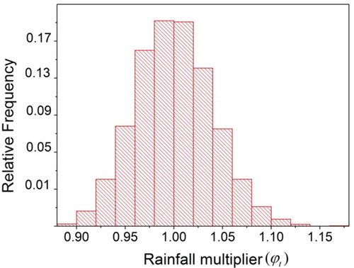
As the possible variation in rainfall is created by the multipliers sampled from the log-normal probability distribution, the initial values of distribution parameters should be appropriate. Hence, the sensitive range of σ, identified to be between 0 and 0.25 by the trial-and-error method, was used as a feasible range in GA. At the end of the optimization, the optimal σ value was found to be 0.03, besides the optimized parameters of the ANN (i.e. weights and biases). The sampling was performed to get multipliers for adjusting the measured rainfall that used the pdf, characterized by the distribution parameters (μ = 1; σ = 0.03). Figure 4 shows the histogram of the multipliers sampled using the optimized pdf. The range of multipliers (i.e. perturbation) was found to vary between 0.85 and 1.15, with a maximum frequency falling close to 1.0 (no error). It is worth mentioning that the “no error” condition was mostly observed for low values of rainfall, and may plausibly be due to the lower error and sensitivity of the rainfall in this domain.

Figure 4. Histogram of rainfall multiplier sampled from the log-normal distribution (Leaf River).

The scatter plot presented in Figure 5 shows the variation of bias (the magnitude of forced error) among the measured values. The results suggest that the bias increases with the magnitude of the rainfall. The mean bias identified for the rainfall is within ±10% in this analysis, which is within acceptable limits (Vrugt et al. 2008).

Figure 5. Two-dimensional scatter plots of observed rainfall vs corrected rainfall.

Model performance

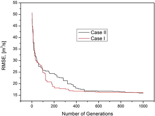
The ability of the model to reproduce the observation was evaluated using various statistical indices: NRMSE, NSE, CC and MBE. The RMSE was used as an objective function to train the ANN model. Figure 6 shows the model convergence towards different generations. During initial generations, the RMSE was high (around 50 m³/s). When the GA progressed in the successive generations, the model showed convergence in both Cases I and II, and an agreed level was reached without any further improvement in the reduction of error.

Figure 6. Convergence of objective function against number of generations.

The mean and standard deviation computed for weights in Case I (input error is not considered) and Case II (input error is considered) are presented in Table 1. The weights of the ANN connecting rainfall inputs to the first and second hidden nodes resulted in significant reduction and increase in mean and standard deviation values, respectively. Similar findings were observed in all other connections (results are not shown here). It may be noted that the weights optimized in parallel computing lead to various magnitudes of weights in neural network modelling. Hence, any different network architecture and input combinations would result in different sets of weight vectors, which require further investigation to reinforce the results.

Table 1. Statistical properties of the ANN parameters optimized for Case I and Case II. SD: standard deviation.

	Case I		Case II
Parameter	Mean	SD	Mean	SD
WI1H1	−7.12	1.74	0.76	0.14
WI1H2	−0.65	0.16	−0.45	0.78
WI2H1	−2.61	2.30	0.48	0.06
WI2H2	−0.25	0.10	−0.79	0.92
WI3H1	−0.34	2.63	0.54	0.15
WI3H2	−0.44	0.07	−2.35	0.86
WI4H1	−2.54	1.53	−0.14	0.16
WI4H2	0.04	0.17	1.03	0.8

The performance indices computed for Cases I and II are presented in Table 2 for model calibration and validation. It is evident from Table 2 that both cases show consistent performance during calibration as well as validation, indicating the absence of overtraining. The MBE values show overestimation in Case I and underestimation in Case II during calibration, and a similar response was found in validation. The high CC values (i.e. more than 0.90 in Cases I and II) indicate a close fit between the predicted and observed values. It is worth mentioning here that the introduction of an error in the measured rainfall resulted in a slightly better (may not be significant) performance in the Case II simulation compared to Case I. A possible reason for such slightly improved performance could be the presence of an actual (potential) error in the measured data used in this study. However, more investigation is required to reinforce this inference.

Table 2. Summary statistics and model performance indices.

	Calibration				Validation
Source of uncertainty	CC	NSE (%)	NRMSE (m^3/s)	MBE (m^3/s)	CC	NSE (%)	NRMSE (m^3/s)	MBE (m^3/s)
Case I	0.93	86.91	0.74	–0.49	0.93	86.25	0.89	–5.32
Case II	0.94	88.14	0.70	2.14	0.94	87.12	0.86	1.95

Parameter uncertainty

The model parameter uncertainty can be defined as a range, which in turn propagates the uncertainty in the model predictions. While a narrow range of parameters indicates a reduced a level of model prediction uncertainty, a wider range can still produce similar model performance without obvious change in the prediction uncertainty, due to the issue of equifinality. Nonetheless, a narrow range is often preferred from the model calibration. Figures 7 and 8 depict the progressive compression of calibrated model parameters along the number of generations in Cases I and II, respectively. Note that the ranges of initial parameter need to be fixed. This study used the range of (–10 to +10) as suggested by Dhanesh and Sudheer (2011). For most of the parameters, the progressive compressive range of parameter was obtained after 500 generations. It is interesting to note that most of the connection weights that connect the second hidden node to all inputs (i.e. WI₁H₂, WI₂H₂, WI₃H₂, WI₄H₂, WI₅H₂, WI₆H₂, WI₇H₂, WI₈H₂, BH₂) had significant compression in Case I, while the connection to the first hidden node showed higher variability even after 500 iterations. On the contrary, in Case II the compressed range of parameters was significant for weights that connect the first hidden node with all the inputs, while the connection to the second hidden node with the rainfall inputs were not converging after a number of generations. These results indicate the effect of error in the rainfall considered in the model calibration in Case II. In addition, it was observed that the introduction of error in the measured rainfall significantly alters the location and shape parameters of each weight vector of the ANN (results are not presented here). In other words, the ANN parameters are highly sensitive to the values of the input variables (Srivastav et al. 2007). It is also to be noted that in both cases some of the parameters did not converge even after 1000 generations, indicating a significant level of associated parameter uncertainty during the model calibration. The presented results indicate that analysing the possible variations in model inputs has a significant impact on the model output, which should not be ignored.

Figure 7. Case I: Variation of parameter range along the number of generations. W: weight parameter; B: bias parameter; I, H and O: input, hidden and output nodes, respectively; subscript i corresponds to the ith node in the respective layer, e.g. WI₁H₂ indicates a weight connection between 1st input and 2nd hidden node.

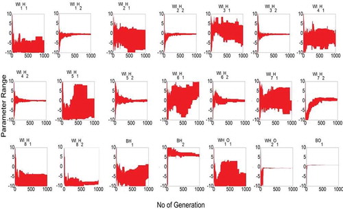
Figure 8. Case II: Variation of parameter range along the number of generations. See Figure 7 for explanation of notation.

Ensemble model simulation and estimation of prediction uncertainty

Ensemble of simulation for quantifying parameter uncertainty of ANN was performed in Stage 2 optimization, such that, the optimal variability in the ANN parameters (i.e. obtained in Stage 1) was identified for constructing the prediction interval. The initial range of perturbation limit was fixed between ± 30%, and population size and number of generations were considered to be 100, 1000 respectively through various trails in the GA. The pareto-optimal front (Fig. 9) was constructed from the ensemble of model simulation obtained using the multi-objective function. 

Figure 9. Pareto-optimal front of optimization during ensemble creation in the calibration period.

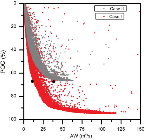
It is very clear from Figure 9 that the Pareto-optimal front obtained from the model calibration is different for the two cases (no overlapping is observed). The Pareto-optimal front has resulted in multiple solutions in Case I, with increased width in the prediction interval. However, in Case II, the Pareto-optimal front was unable to progress along the x-axis beyond some point, which indicates the influence of including input error. Overall, the results suggest that any error in the input will significantly affect the acceptably of the models, as is evident from the uncertainty indices corresponding to the Pareto-optimal front in Case II. It is noted that each point refers to the ensemble of simulation obtained during Stage 2.

Two points (indicated as dots) from the converged envelope of the Pareto-optimal front were selected to compare the effect of input error: one from the (red) optimal front (Case I) and one from the (grey) optimal front (Case II). The prediction uncertainty of the model corresponds to the selected points, as presented in Table 3. It may be noted that the quality of the prediction interval is based on including the maximum number of observations within the prediction interval, whose width is also minimized. Accordingly, those points were selected that have equal values of POC in order to analyse the magnitude of the average width of the prediction interval, and thus the prediction uncertainty can be compared. It is clear from Figure 9 that, for equal values of POC (around 60%), the average width of the prediction interval obtained for Cases I and II is different. In the case of ensemble simulation that did not consider any input error (Case I), an AW of 12.88 m³/s was obtained, while the ensemble that considered input error in model calibration (Case II) had an AW of 38.23 m³/s. In the model validation, a slightly higher level of uncertainty was observed, with POC = 53.84% and AW = 66.09 m³/s for the ensemble selected from Case II, as compared to that selected for Case I (POC = 62.45% and AW = 49.92 m³/s). Figures 10 and 11 confirm the increase in magnitude of the prediction interval width obtained for Case II in the calibration and validation stages, respectively. For brevity, only a portion of the calibration period (20 December 1954 to 7 July 1955) is presented in Figure 10, and of the validation period (13 March 1961 to 28 September 1961) in Figure 11.

Table 3. Uncertainty indices estimated for Case I and Case II. POC: percentage of coverage; AW: average width.

	Case I		Case II
Measures	Calibration	Validation	Calibration	Validation
POC (%)	60.48	62.45	60.54	53.84
AW (m^3/s)	12.88	49.92	38.23	66.09

Figure 10. Prediction interval corresponding to selected ensemble during the calibration period.

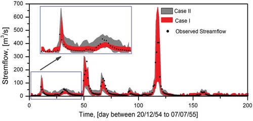
Figure 11. Prediction interval corresponding to selected ensemble during the validation period.

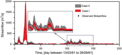
While it is evident from Figures 10 and 11 that the uncertainty interval contains many of the observed streamflow values in both Cases I and II, the observed values were close to the lower bound of the uncertainty interval in the low-flow season. This shows a slight overestimation of low flow by the ANN models; in particular, this was observed in Case II, where some of the low flows were not contained within the prediction interval. It is also evident that the prediction interval obtained in Case II has large average width in both low- and medium-flow ranges compared to the interval estimated in Case I. However, in the case of high-flow series, no distinct variability was observed in the width of the prediction interval for both Cases I and II, which suggests a similar level of uncertainty. This may be due to the fact that the forced error at higher magnitude of rainfall is insignificant compared to the magnitude of the rainfall (±10%).

Despite the similar model performance in terms of accuracy (Table 1), the level of uncertainty increased when input error was included during model calibration as well validation (Figs. 10 and 11). This information suggests the need for a detailed analysis of uncertainty by explicitly considering different sources of uncertainty during modelling.

Summary and conclusions

The quantification of input uncertainty in an ANN model was proposed and illustrated through rainfall–runoff modelling, in the Leaf River watershed. In Stage 1 of the optimization, the plausible realization of errors was sampled from a probabilistic distribution and applied to measured rainfall. In Stage 2 of the optimization, the parameter uncertainty of the ANN was quantified in terms of constructing the prediction interval. To demonstrate the influence of input error, the model was compared with one that used input without error in the model calibration. It was found that calibration of model parameters by incorporating the input uncertainty improves the understanding of the ANN model behaviour, with possible variability in the model prediction and with slight improvement in the model prediction. The approach proposed in this paper provides useful information that could be used for testing hydrological theory, diagnosis of model error, and maximizing the chances of appropriate parameter values. This information could be further used for verifying spatial variations in raingauge measurements, and correcting errors in rainfall measured using radar techniques. Overall, the method proposed for the input uncertainty is simple to apply in ANN models with a minimum number of parameters, which in turn ensures a reduction in any additional source of uncertainty without compromising the model performance.

Scope for further research

It may be noted that each uncertainty method in the literature has its own principle and assumptions, thus cannot be directly applied without modifications. It is suggested that application of methods such as BATEA and DREAM in ANN models would be useful in comparing the results and verifying the validity of different uncertainty methods. Initially, the problem was formulated as a single-stage optimization including all parameters as decision variables. However, our experience was that the optimization algorithm does not converge even with a large number of generations. One reason for this could be the difficulty in assuming an initial range of ANN parameters, unlike other conceptual and physically-based models in which the initial range of model parameters is usually known. Nonetheless, combining the first and second optimization steps together can have certain advantages when using recent developments in optimization techniques, such as the hybrid optimization algorithm. The presented study is limited to eight input variables. However, if the number of inputs is increased and if multiple outputs are considered, the model will be computationally intensive, and might lead to a local minima problem. Hence further research is required to make strong conclusions. It is well known that rainfall has a significant amount of uncertainty as compared to other variables. Due to this fact, this study is limited to considering the uncertainty of rainfall input alone. However, analysing uncertainty in all the inputs might result in more realistic sets of model parameters and meaningful quantification of model prediction uncertainty.

Disclosure statement

No potential conflict of interest was reported by the authors.

References

- Burnash, R.J.C., Ferral, R.L., and McGuire, R.A., 1973. A generalized stream flow simulation system. In: Concerned modelling for digital computers. Sacramento, CA: Joint Federal–State River Forecast Centre.
- Chang, F.-J., Chiang, Y.-M., and Chang, L.-C., 2007. Multi-step-ahead neural networks for flood forecasting. Hydrological Sciences Journal, 52 (1), 114–130. doi:10.1623/hysj.52.1.114
- Dawson, C.W., Abrahart, R.J., and See, L.M., 2007. HydroTest: A web-based toolbox of evaluation metrics for the standardised assessment of hydrological forecasts. Environmental Modelling & Software, 22 (7), 1034–1052. doi:10.1016/j.envsoft.2006.06.008
- Deb, K., et al., 2002. A fast and elitist multi-objective genetic algorithm: NSGA-II. IEEE Transactions on Evolutionary Computation, 6 (2), 182–197. doi:10.1109/4235.996017
- Dhanesh, Y. and Sudheer, K.P., 2011. Predictions in ungauged basins: can we use artificial neural networks? American Geophysical Union Joint Assembly, Foz do Iguassu, Brazil, August 8–13, 2010.
- Ebtehaj, M., Moradkhani, H., and Gupta, H.V., 2010. Improving robustness of hydrologic parameter estimation by the use of moving block bootstrap resampling. Water Resources Research, 46, 1–14. doi:10.1029/2009WR007981
- He, J., Anderson, A., and Valeo, C., 2015. Bias compensation in flood frequency analysis. Hydrological Sciences Journal, 60, 381–401. doi:10.1080/02626667.2014.885651
- Hsu, K., Gupta, H.V., and Sorooshian, S., 1995. Artificial neural network modeling of the rainfall–runoff process. Water Resources Research, 31 (10), 2517–2530. doi:10.1029/95WR01955
- Kasiviswanathan, K.S., et al., 2013. Constructing prediction interval for artificial neural network rainfall runoff models based on ensemble simulations. Journal of Hydrology, 499, 275–288. doi:10.1016/j.jhydrol.2013.06.043
- Kavetski, D., Kuczera, G., and Franks, S.W., 2006. Bayesian analysis of input uncertainty in hydrological modeling: 2. Application. Water Resources Research, 42, W03408. doi:10.1029/2005WR004376
- Kumar, A.R.S., et al., 2005. Rainfall-runoff modelling using artificial neural networks: comparison of network types. Hydrological Processes, 19 (6), 1277–1291. doi:10.1002/(ISSN)1099-1085
- Kumar, M., Raghuwanshi, N.S., and Singh, R., 2002. Estimating evapotranspiration using artificial neural network. Journal of Irrigation and Drainage Engineering, 128, 224–233. doi:10.1061/(ASCE)0733-9437(2002)128:4(224)
- Li, Y., et al., 2015. Parametric uncertainty and sensitivity analysis of hydrodynamic processes for a large shallow freshwater lake. Hydrological Sciences Journal, 60 (6), 1078–1095. doi:10.1080/02626667.2014.948444
- Maier, H.R., et al., 2010. Methods used for the development of neural networks for the prediction of water resource variables in river systems: current status and future directions. Environmental Modelling & Software, 25, 891–909. doi:10.1016/j.envsoft.2010.02.003
- Nayak, P.C., et al., 2005. Short-term flood forecasting with a neurofuzzy model. Water Resources Research, 41, 1–16. doi:10.1029/2004WR003562
- Nestor, L.S.Y., 2006. Modelling the infiltration process with a multi-layer perceptron artificial neural network. Hydrological Sciences Journal, 51 (1), 3–20. doi:10.1623/hysj.51.1.3
- Parasuraman, K. and Elshorbagy, A., 2008. Toward improving the reliability of hydrologic prediction: model structure uncertainty and its quantification using ensemble-based genetic programming framework. Water Resources Research, 44, 1–12. doi:10.1029/2007WR006451
- Patil, A. and Deng, Z.-Q., 2012. Input data measurement induced uncertainty in watershed modelling. Hydrological Sciences Journal, 57 (1), 118–133. doi:10.1080/02626667.2011.636044
- Sorooshian, S., Duan, Q., and Gupta, V.K., 1993. Calibration of rainfall–runoff models: application of global optimization to the Sacramento Soil Moisture Accounting model. Water Resources Research, 29, 1185–1194. doi:10.1029/92WR02617
- Srivastav, R.K., Sudheer, K.P., and Chaubey, I., 2007. A simplified approach to quantifying predictive and parametric uncertainty in artificial neural network hydrologic models. Water Resources Research, 43, 1–12. doi:10.1029/2006WR005352
- Sudheer, K.P., Gosain, A.K., and Ramasastri, K.S., 2002. A data-driven algorithm for constructing artificial neural network rainfall–runoff models. Hydrological Processes, 16, 1325–1330. doi:10.1002/hyp.554
- Tiwari, M.K., et al., 2013. Improving reliability of river flow forecasting using neural networks, wavelets and self-organising maps. Journal of Hydroinformatics, 15 (2), 486–502. doi:10.2166/hydro.2012.130
- Tolson, B.A. and Shoemaker, C.A., 2007. Dynamically dimensioned search algorithm for computationally efficient watershed model calibration. Water Resources Research, 43, W01413. doi:10.1029/2005WR004723
- Vrugt, J.A., et al., 2003. A Shuffled Complex Evolution Metropolis algorithm for optimization and uncertainty assessment of hydrologic model parameters. Water Resources Research, 39 (8), 1201. doi:10.1029/2002WR001642
- Vrugt, J.A., et al., 2008. Treatment of input uncertainty in hydrologic modeling: doing hydrology backward with Markov chain Monte Carlo simulation. Water Resources Research, 44, 1–15. doi:10.1029/2007WR006720
- Vrugt, J.A., et al., 2009. Equifinality of formal (DREAM) and informal (GLUE) Bayesian approaches in hydrologic modeling? Stochastic Environmental Research and Risk Assessment, 23, 1011–1026. doi:10.1007/s00477-008-0274-y
- Ye, L., et al., 2014. Multi-objective optimization for construction of prediction interval of hydrological models based on ensemble simulations. Journal of Hydrology, 519, 925–933. doi:10.1016/j.jhydrol.2014.08.026
- Yen, H., et al., 2015. Assessment of input uncertainty in SWAT using latent variables. Water Resources Management, 29, 1137–1153. doi:10.1007/s11269-014-0865-y
- Zhang, X., et al., 2009. Estimating uncertainty of streamflow simulation using Bayesian neural networks. Water Resources Research, 45, 1–16. doi:10.1029/2008WR007030
- Zhang, X., et al., 2011a. Explicitly integrating parameter, input, and structure uncertainties into Bayesian Neural Networks for probabilistic hydrologic forecasting. Journal of Hydrology, 409, 696–709. doi:10.1016/j.jhydrol.2011.09.002
- Zhang, X.Y., et al., 2011b. Structural uncertainty assessment in a discharge simulation model. Hydrological Sciences Journal, 56 (5), 854–869. doi:10.1080/02626667.2011.587426