Real-time assimilation of streamflow observations into a hydrological routing model: effects of model structures and updating methods

ABSTRACT

This paper comparatively assesses the performance of five data assimilation techniques for three-parameter Muskingum routing with a spatially lumped or distributed model structure. The assimilation techniques used include direct insertion (DI), nudging scheme (NS), Kalman filter (KF), ensemble Kalman filter (EnKF) and asynchronous ensemble Kalman filter (AEnKF), which are applied to river reaches in Texas and Louisiana, USA. For both lumped and distributed routing, results from KF, EnKF and AEnKF are sensitive to the error specification. As expected, DI outperformed the other models in the case of lumped modelling, while in distributed routing, KF approaches, particularly AEnKF and EnKF, performed better than DI or nudging, reflecting the benefit of updating distributed states through error covariance modelling in KF approaches. The results of this work would be useful in setting up data assimilation systems that employ increasingly abundant real-time observations using distributed hydrological routing models.

KEYWORDS:

• hydrological routing
• data assimilation
• three-parameter Muskingum model
• distributed routing

Editor A. Castellarin Associate editor G. Thirel

1 Introduction

River routing is critical in real-time hydrological forecasting operations in order to mitigate losses and damages by informing on the correct timing of floods. Since the development of the Muskingum method by McCarthy (1938), hydrological routing models have been used extensively due to their parsimony and minimal data and computational requirements (O’Donnell 1985, Boku and Xuewei 1987, Georgakakos et al. 1990, Samani and Jebelifard 2003, Barbetta et al. 2011, Xu et al. 2012, Haddad et al. 2015, Yuan et al. 2016). Moreover, these models can replace complicated hydraulic models when river cross-section data are unavailable. However, due to simplifying assumptions, hydrological routing is subject to potentially significant structural and parametric errors. To address this, data assimilation (DA) approaches have increasingly been used to optimally update model input, states, parameters and/or outputs in order to reduce model uncertainty and improve predictions (WMO (World Meteorological Organization) 1992, Refsgaard 1997, McLaughlin 2002, Moradkhani et al. 2005a, Walker and Houser 2005, Liu and Gupta 2007, Reichle et al. 2008). It is also noteworthy that types of uncertainty in models and observations can be categorized into two sources: aleatory (random) and epistemic (of unknown character, nonrandom) (Beven 2016). Measurement errors in rainfall and water level observations can be considered as aleatory uncertainty, while epistemic uncertainty sources include parametric and model structural uncertainties.

Applications of hydrological DA in surface water modelling can largely be divided into DA on rainfall–runoff modelling and river routing. For DA on rainfall–runoff modelling, it is common that hidden (latent or unobserved) state variables (e.g. soil moisture, evapotranspiration, snow water equivalent, runoff and discharge states) and/or associated parameters are updated by observation of measurable quantities, e.g. streamflow (Pauwels and De Lannoy 2006, 2009, Weerts and El Serafy 2006, Noh et al. 2013), water depth (Madsen and Skotner 2005, Neal et al. 2007), soil moisture (Brocca et al. 2010, 2012), and snow cover (Andreadis and Lettenmaier 2006). For DA on routing, the variables (e.g. streamflow and/or water depth) updated in the measurement equations are usually identical to those in state-space equations. It is worth mentioning that, in hydrological applications, both states and parameters can be included in the control vector for DA, as described in Moradkhani et al. (2005b), DeChant and Moradkhani (2012) and Moradkhani et al. (2012). Features of streamflow DA are also discussed in Sun et al. (2016).

Compared to various applications of DA on hydraulic or hydrodynamic routing (Madsen et al. 2003, Andreadis et al. 2007, Neal et al. 2007, 2009, 2012, Matgen et al. 2010, Biancamaria et al. 2011, Giustarini et al. 2011, Jean-Baptiste et al. 2011, Ricci et al. 2011, García-Pintado et al. 2013, Kim et al. 2013a, 2013b, Andreadis and Schumann 2014; Barthelemy, et al. 2017), DA on hydrological routing has received little attention. This is probably due to the assumption that conventional DA methods for linear systems, such as Kalman filtering, are sufficient for hydrological routing. Therefore, a comprehensive evaluation of the effect of various DA methods on hydrological routing has not been carried out thoroughly. Seo et al. (2003) improved the estimate of distributed hydraulic parameters of a kinematic wave routing model by assimilating streamflow observations using a variational method. Liu et al. (2008) used a one-dimensional variational (1D-VAR) method to integrate streamflow observations within a three-parameter Muskingum model.

In addition, the effects of different uncertainty specifications on flood predictions are hardly known, despite an obvious demand for improved real-time forecasting in real-world applications. In order to derive recommendations about DA methods that work well for given model structures, the evaluation efforts should take into account different model structures and different river systems.

The aim of this study is to assess the effect of different DA methods on streamflow predictions with two different structures (i.e. lumped and distributed) of a three-parameter Muskingum hydrological routing model. The five different DA methods selected for this study are direct insertion (DI), nudging scheme (NS), Kalman filter (KF), ensemble Kalman filter (EnKF) and asynchronous ensemble Kalman filter (AEnKF). Different error specifications are used for the different model structures and DA methods (e.g. deterministic and ensemble Kalman filter methods). In the case of lumped routing, the effect of different DA methods is compared via updating a state variable (streamflow discharge) at the downstream boundary location, using observations from a single location; while in the case of distributed routing, the assimilation points are located both within the river reach and at the downstream boundary location. The simulation experiments are implemented for three different river reaches located along the Trinity and Sabine rivers, Texas, USA. The effect of different estimations of model error in ensemble-based assimilation methods is also investigated.

The paper is organized as follows. First, we describe the three-parameter Muskingum model together with the assimilation approach (Section 2). In Section 3, the case study is described; we define the different experimental set-ups in Section 4; and, finally, the results and conclusions are given in Section 5.

2 Methodology

To evaluate the performance of hydrological routing models, the different DA methods include three deterministic (DI, NS and KF) and two probabilistic (EnKF and AEnKF) methods, which are evaluated by both deterministic and probabilistic measures. Among various hydraulic and hydrological models, the Muskingum-based hydrological routing is chosen, not only because of minimal data and computational requirements, but also because of increasing applications of hydrological routing in real-time forecasting and large-scale modelling (Gochis et al. 2015, Rakovec et al. 2016).

2.1 The three-parameter Muskingum model

A three-parameter Muskingum model (3p-Musk; O’Donnell 1985) is implemented in order to represent downstream flood propagation:

(1)

where n and t are the space and time indexes, respectively. In Equation (1), C₁, C₂ and C₃ are the model coefficients, estimated as:

(2)

where K₁ and K₂ are the model parameters representing the weighting factor and the storage constant (h), respectively. The derivation of the 3p-Musk model is based on the standard formulation of the Muskingum model (Todini 2007). Georgakakos et al. (1990) proposed a stochastic state-space form of the Muskingum model:

(3)

where x is the n_state × 1 model state matrix (streamflow in m³/s) related to each river section including the outflow, in which n_state denotes the number of discrete reaches that the river is divided into; I_t is the 2 × 1 input vector of the discharge at the upstream boundary condition (Georgakakos et al. 1990); and w_t is the model structural uncertainty expressed as normal distribution with zero mean and covariance S at time t. The matrices Ф (n_state × n_state) and Γ (n_state × 2) represent the state-transition and input-transition matrices, respectively, and are functions of three model coefficients C₁, C₂ and C₃, derived based on Equation (1) (Georgakakos et al. 1990). In the measurement equation, the matrix z_t (n_obs × 1), representing the flow along the river channel at time t, is expressed as:

(4)

where v_t is the measurement error expressed as normal distribution, with zero mean and covariance R; and H (n_obs × n_state) is the output matrix which, for a given observation, is equal to 1 at the outlet location and zero elsewhere. However, in the original Muskingum model, no lateral inflow or outflow along the reach is considered. O’Donnell (1985) presented a direct and efficient method to extend the two-parameter Muskingum model to a three-parameter model by accounting for the lateral inflow, which is modelled as upstream inflow multiplied by K₃. The new set of coefficients d₁, d₂ and d₃ are estimated as:

(5)

If there is no lateral inflow, K₃ = 0 and d₁, d₂ and d₃ reduce to the coefficients C₁, C₂ and C₃ in Equation (2).

2.2 Data assimilation

State estimation methods are widely applied tools in hydrology that efficiently use observational information to improve model predictions and reduce modelling uncertainty (McLaughlin 1995, 2002, Refsgaard 1997, Madsen and Skotner 2005). Recently, Liu et al. (2012) presented a comprehensive literature review of the latest advances in data assimilation procedures in operational flood forecasting that have been achieved by assimilating water observations from in situ sensors or remote sensing in a distributed fashion. In this study, DI, NS, KF, EnKF and AEnKF are used as described below. It is worth noting that only model states (river flow) are updated in this study, while the model parameters are constant along the simulation windows. For the lumped model structure, there is one model state, which is discharge at the downstream location and is updated using flow measurement data at the same location. For the distributed structure, model states of all river reaches are updated using measurements from multiple gauging locations. Because DA combines observational and model information to provide an estimate of the most likely state and its uncertainty (Lahoz and Schneider 2014), statistical information on observations could be used to analyse the performance of DA methods, which is discussed in Section 2.4.

2.2.1 Direct insertion

In DI, also known as the Cressman method (Daley 1991), the model states are directly replaced with the observations, whenever available:

(6)

where z^o and x are the observation value and the updated model state at time step t at a particular location l. Updated state values are indicated with the superscript +. The main statistical hypothesis (and limitation) of this method is that measurements are considered exact and reliable and that the model contains no information (Refsgaard 1997). However, the risk of this approach, as in the case of the Kalman filter-based approaches, is that unbalanced state estimates can be obtained, which causes model shocks (Walker et al. 2001).

2.2.2 Nudging scheme

The NS technique consists of adding a nudging or innovation term in the model update equation in order to “force” the model state to be closer to the observations (Brocca et al. 2010). The nudging term is proportional to the difference between the model states, and the observations calculated at a given location. The general formulation of NS is:

(7)

where K is the nudging (or gain) matrix estimated as:

(8)

where S_t and R_t are the model and observational error variance, respectively, at the time step t. The superscript − indicates the predicted matrices. In the case of perfect measurement R_t = 0, K = 1 and x⁺ = z^o, as in the DI approach. Alternatively, if the model is assumed perfect, S_t = 0 and K = 0, which means that there will be no update (free run) since x⁺ = x⁻. Although NS is not statistically optimal (Brocca et al. 2010), it can be used to assimilate streamflow observations with low computational time costs. A detailed review of nudging methods is presented by Park and Xu (2013).

2.2.3 Kalman filter

The Kalman filter (KF; Kalman 1960) is a mathematical stochastic tool which allows the estimation, in an efficient optimal recursive way, of the state of a process governed by a linear stochastic difference equation as a response to real-time (noisy) observations. The KF procedure can be divided into two steps: forecasting and updating. The forecasted (with superscript −) model state matrix is estimated based on Equation (1), while the forecasted model covariance matrix P (n_state ×  n_state) is expressed as:

(9)

The prior model states x at time t are updated (with superscript +), as the response to the new available observations, using the following equations:

(10)

(11)

(12)

where K_t is the n_state × n_obs Kalman gain matrix. Because nonlinear-dynamic models are favoured by model developers and users, KF is not applied extensively in the hydrological community. In addition, another limitation in the implementation of KF is the subjective determination of model errors, as underlined in Mazzoleni (2017). On one hand, the confidence in the model can be reduced if the model error is overestimated, while, on the other hand, too much trust in the model can be achieved if the model error is underestimated, and the information from the new observations discarded (Kitanidis and Bras 1980, Sun et al. 2016). Puente and Bras (1987) argued that the proper error quantification of the model is even more important than the selection of the DA methods.

Different (subjective) methods have been proposed to calculate a model error for KF, as reported in Maybeck (1982) and Mazzoleni (2017). One of the main challenges of model error estimation is the computational costs required for large models. In addition, simple parameterization of the model error might be necessary due to the lack of available information (Dee 1995). Hence, in most of the applications with KF, the common approach is to manually calibrate the model error (Verlaan 1998). Another approach is to use the least squares method to minimize the difference between the computed and observed covariance of the residuals (Verlaan 1998).

2.2.4 Ensemble Kalman filter

For nonlinear systems, the EnKF (Evensen 2009) can be used to overcome the limitation of the linearity assumption used for KF. The EnKF (Reichle et al. 2002, Evensen 2003, Weerts and El Serafy 2006; Noh et al. 2013) is widely used in hydrological applications, and defines model error as a function of the spread of the model state ensemble. In the stochastic formulation of EnKF, the vector of the forecasted (or background) ensemble of model states x is represented as:

(13)

where i is the given ensemble member and N_ens is the total number of ensemble members. The model error covariance matrix P is calculated as proposed by Evensen (2003):

(14)

where E is the ensemble anomaly (Clark et al. 2008) for each ensemble member:

(15)

A perturbed (with noise v_t) normally distributed measurement vector z^o is generated when a new observation becomes available. As in the case of KF, the updated model state matrix is estimated using Equation (11), assimilating each member of the observation ensemble vector z (see Section 2.4) with a member of the forecasted model state matrix and using Equation (10) to estimate the Kalman gain K.

The EnKF can be used to replace KF if the dimension of the state matrix is large and if a non-linear model structure is used. Theoretically, in the case of linear dynamics and Gaussian noise, EnKF should converge to the KF solution. However, according to different uncertainty specifications, KF-based methods can lead to different solutions, as discussed in Section 5. One of the reasons to apply EnKF, even for a linear system, is primarily that the estimation of model error in EnKF is less subjective than in KF. In fact, in EnKF, the filter parameters can be calibrated using rigorous approaches such as the one proposed by Anderson (2001).

2.2.5 Asynchronous ensemble Kalman filter

The AEnKF, a generalization of the EnKF introduced by Sakov et al. (2010), uses past observations over a time window at once to update the model states at the current time step (Rakovec et al. 2015). Unlike 4D-VAR, AEnKF does not require any adjoint models. The model state matrix is augmented with the past observations from the W previous time step. While EnKF updates the model using the observation at the current time step t, AEnKF uses the past as well as current observations at time steps from t − W to t. The new state augmented matrix (n_state+W × 1) can be expressed as:

(16)

where H(x_t−W,i) is the model output corresponding to the time step t − W. In a similar way, with the new state definition, also the operator matrix H (n_state + W × n_state + W), the observation covariance matrix R (n_obs + W × n_obs + W) and the observation vector z (n_obs + W × 1), can be expressed in their augmented form as:

(17)

(18)

(19)

where I is the identity matrix having the same dimension of H, i.e. (1 × n_state). It is worth noting that, even if the matrices are made by augmenting with past observations, Equation (16) is solved only for the current time step t without updating past model states. Following Equations (10) and (14), the matrices K and P also change their sizes in both rows and columns. In fact, an extra column in K corresponds to the gain due to one past observation. If W = 0, AEnKF is identical to EnKF. The characteristic of the AEnKF of adding past observations to improve the DA procedure at the current time step is very attractive for operational use, given its relatively small computational costs. It is worth mentioning that the AEnKF method differs from a Kalman smoother approach because AEnKF uses past observations to update only the states at time step t, while the smoother approaches also update past model states.

2.3 Model error estimation

The proper model error estimation is fundamental in order to properly implement DA techniques and improve model output. The estimation of model error for each of the methods employed (deterministic DA: DI, NS and KF; ensemble-based DA: EnKF and AEnKF) is reported below.

2.3.1 Deterministic DA methods

Model error estimation is not required for DI. However, for NS and KF, the covariance matrix S is initially estimated as a diagonal matrix (n_state × n_state) where the covariance of the observed and simulated streamflow is used as the diagonal elements of S. See Sections 3 and 4 for further details.

2.3.2 Ensemble-based DA methods

The EnKF and AEnKF methods are Monte Carlo approximations of a sequential Bayesian filtering process, which alternates between an ensemble forecast step and a state variable update step. In the forecast step, an ensemble of model states is propagated forward in time using the model. As a result, the accuracy of the sampled covariances depends on the model perturbation and ensemble size (Equations (17) and (18)). That is why it is extremely important to properly assess the spread of the ensemble for both EnKF and AEnKF.

In EnKF and AEnKF, the boundary I (i.e. river flow) is perturbed as follows:

(20)

where I′ is the ensemble of perturbed boundary conditions at time t, U is the uniform distribution, and ε_I is the input hyper-parameter. It is worth noting that model parameters are not perturbed in this study. In fact, we found that perturbing model parameters with high hyper-parameter values leads to instability in the distributed 3p-Musk model. For this reason, only boundary I is perturbed for both lumped and distributed model structures. Two different approaches are used to generate the model ensemble.

2.3.2.1 Identical model error variance approach (sub-opt)

In the case of the lumped model, the model ensemble is generated by perturbing the model parameters in such a way that the variance of the ensemble spread is equal to the value of S, estimated for NS and KF. However, in this case the EnKF is sub-optimal because the filter parameters, and the consequent ensemble spread, are not properly calibrated following the approach proposed by Anderson (2001).

2.3.2.2 Optimized model error variance approach (optimal)

Because of the filter sensitivity to model error definition, the tuning of the process noise value is the key factor to properly compare the different DA methods (Brochero et al. 2011, Abaza et al. 2015). A subjective variation of S in the KF might provide better or worse results if compared to an optimal EnKF, compromising the correctness and reliability of the study. In this study, we use the method proposed by Abaza et al. (2014, 2015) to estimate the ε_I value, which led to a normalized root mean square error ratio (NRR) close to one. In fact, the optimal ensemble generates a NRR value equal to 1; NRR > 1 indicates small ensemble spread and NRR < 1 indicates the opposite.

2.4 Estimation of the observational error

The proper characterization of the observational covariance error R_t is very important because it directly affects the DA performance. In this study, (R_t)^1/2 is assumed to be linearly dependent on the observed flow z^o at a given measurement location:

(21)

where the proportionality coefficient α_t is set to 0.1 for each time step, as suggested by Weerts and El Serafy (2006), Clark et al. (2008) and Rakovec et al. (2012).

For EnKF and AEnKF, an ensemble of observed streamflow observations z_t, normally distributed, with mean z_t^o and covariance R_t, is generated as follows:

(22)

2.5 Performance measures

2.5.1 Deterministic measures

The performance of DA is measured by the Nash-Sutcliffe efficiency (NSE; Nash and Sutcliffe 1970), and bias index (Bias).

The NSE compares simulated and observed time series by:

(23)

where Q_t^m and Q_t^o are the simulated and observed streamflow in the tth time step, respectively; is the average observed streamflow; and T is the number of pairs of simulated and observed streamflow. A value of NSE = 1 represents a perfect model simulation, while NSE = 0 indicates that the simulated streamflow is as accurate as the mean of the observed streamflow.

The Bias measures the tendency of the total simulated streamflow to be larger or smaller than the observed one:

(24)

Values greater than 1 indicate overestimation of the streamflow and overall underestimation otherwise.

2.5.2 Probabilistic measures

Four different probabilistic measures are used in this study: Brier skill score (BSS, Richardson 2001, Weigel et al. 2007), continuous ranked probability score (CRPS, Bröcker 2012), receiver operating characteristic curve (ROC, Hajian-Tilaki 2013) and reliability diagram (Brochero et al. 2011)

The BSS is a normalized measure of the mean-square error of probability forecasts for two events. A BSS of 1.0 represents a perfect forecast, while BSS = 0.0 indicates the skill of the reference forecasts. Similarly, the CRPS is equivalent to the mean absolute error in deterministic forecasts. CRPS = 0.0 indicates the perfect score (Brochero et al. 2011).

The ROC curve is used to evaluate the ability of a forecast to discriminate the occurrence of a certain event (Trambauer et al. 2015). For example, a hydrograph can be split into two categories: one identifying a flood event (Category 1) and the other corresponding to the non-flood event (Category 0). Where A is the fraction of truly negative events (non-flood events) correctly classified as negative, and B is the fraction of truly positive events (flood events) correctly classified as positive, the ROC curve is a graphical representation of (1 − A) vs B. A perfect discrimination ability will therefore be represented by two perpendicular lines intersecting at the point (1,1). The most important statistical property that can be extracted from the ROCcurve is the area under the curve (AUC). A value of AUC = 1 represents perfect discrimination ability, while a value of 0.5 represents no discrimination ability.

The reliability diagram is used to examine the reliability of a probabilistic or ensemble forecast of binary categorical events (Murphy and Winkler 1987, Franz and Hogue 2011). For example, a hydrograph can be split into two categories: one identifying a flood event (Category 1) and the other corresponding to the non-flood event (Category 0). In this case, the reliability diagram will be a plot of the forecasting frequency of a certain event (x-axis) against the observed event frequency (y-axis). If the forecasting and the observed frequency match, all the points in the reliability diagram will be on the 1:1 diagonal line, also referred to as the perfect reliability line. The closer the points are to the perfect reliability line, the higher the reliability of the probabilistic forecast is.

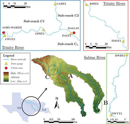
2.6 The Trinity and Sabine Rivers

Comparison of DA methods on hydrological routing was implemented for two rivers in Texas and Louisiana, USA, which are located within the Forecasting domain of the NOAA West Gulf River Forecast Center. With increasing variability of climate and urbanization, these regions are considered flood-prone areas, having experienced devastating floods in recent years (Earl and Vaughan 2015, Schumann et al. 2016).

The Trinity River in north Texas is 1140 km long, with a drainage area of about 46 500 km², 21 major reservoirs, and an average discharge of about 180 m³/s (USGS 2016). The highly dense urbanized area of the Dallas–Fort Worth (DFW) Metroplex area (7 233 323 inhabitants) is located in the upper part of the Trinity River. A major flood that occurred in 1908 resulted in economic losses of about US$5 million and left 4000 people homeless (Barth et al. 2014). Recently, smaller floods have occurred, in May and June 2015.

The Sabine River is a transboundary river between the states of Texas and Louisiana (see Fig. 1). It has a drainage area of about 25 270 km² (76% in Texas and 24% in Louisiana; Phillips 2008). In the recent flood event of January 2016, the Sabine River (on the east Texas side) was hit by a month-long flood.

Figure 1. Trinity and Sabine rivers with the locations of the USGS flow stations.

Flow data for the period 2007–2015 at 15-min time steps are available from monitoring stations, managed by the US Geological Survey (USGS), along the Trinity and Sabine Rivers.

2.7 Model structure

For the purposes of this study, two reaches of the Trinity River and one reach of the Sabine River (see Fig. 1 and Table 1) and two model structures (lumped and distributed) are considered. In particular, for Reach A (between the RSRT2 upstream station and the TDDT2 downstream station) and Reach B (between the BWRT2 upstream station and the DWYT2 downstream station), a lumped version of the 3-par Musk model with n_state = 1 is used. For Reach C, both lumped and distributed model structures are considered. For this purpose, Reach C is divided into sub-reaches C1 (FWOT2 as upstream boundary condition), C2 (CART2 as upstream boundary condition) and C3 (DALT2 station at Dallas used to compare observed and simulated streamflow). The confluence of C1 and C2 is used as the upstream boundary conditions for sub-reach C3. For the distributed structure, a distributed hydraulic model with Δt (s) = 0.9. Δx (m) and n_state = L_reach/Δx is used, where L_reach is the reach length (reported in Table 1) and Δx is the spatial increment implemented along reach C (set to 1000 m). The lumped model structure is implemented considering L_reach = Δx for C1, C2 and C3.

Table 1. Length, in m, of each reach in the Trinity and Sabine rivers.

Reach A	Reach B	Sub-reach C1	Sub-reach C2	Sub-reach C3
78 000	88 000	76 000	30 000	6 000

The main advantage of a distributed formulation over a lumped one is that it is possible to estimate flow characteristics at different points along the reach. For operational applications, it is important to estimate flow values at particular prediction points within urbanized areas, and assimilate flow observations to better predict future flood situations and reduce the consequent economic losses.

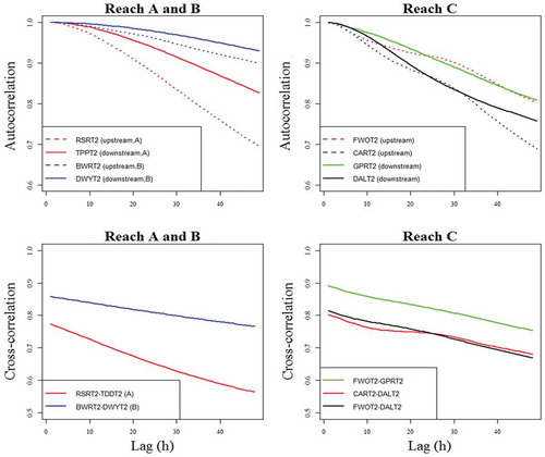
Figure 2 shows auto- and cross-correlation of streamflow observations for simulation periods. For both reaches A and B, as the lag time increases, autocorrelation decreases faster at the upstream locations (RSRT2, BWRT2) than at the downstream ones (TPPT2, DWYT2), which illustrates higher persistency of flows at the downstream to remain in the same state from one observation to the next. Values of both auto- and cross-correlation are consistently higher at Reach B over Reach A for all lag times. In Reach C, the difference of autocorrelation between upstream and downstream is not shown clearly, partly because the simulation period is relatively short. However, the impact of merging two upstream reaches is shown in the cross-correlation plot; values of cross-correlation among two upstream locations (FWOT2, CART2) and one downstream location (DALT2) are lower than those between FWOT2 and GPRT2, which are located at the same sub-reach (C1) before merging with another upstream sub-reach (C2). Due to the nature of simple DA methods such as DI and NS, the performance of these methods can be dependent on the magnitude of auto- and cross-correlation of observations, which is discussed with experimental results in Section 5.

Figure 2. Auto- and cross-correlation of streamflow observations.

2.8 Model calibration and validation

2.8.1 Reaches A and B

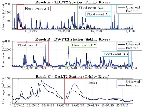
Calibration for the lumped 3p-Musk model implemented in reaches A and B is performed in Lee et al. (2011), by means of the least squares minimization technique using the Broyden-Fletcher-Goldfarb-Shanno variant of the Davidon-Fletcher-Powell minimization (DFPMIN) algorithm (Press et al. 1992) belonging to the class of quasi-Newton methods. The optimal parameter values estimated for the two reaches in the Trinity and Sabine rivers are reported in Table 2. In fact, the higher parameter values in reaches A and B are justified by the fact that parameters refer to the whole river reach, while those for Reach C (distributed routing) refer to the single spatial discretization. That is why the storage constant (K₂) and distributed lateral inflow (K₃) are smaller in the case of distributed routing compared to the lumped modelling. Validation of the lumped hydraulic model is performed by comparing five years (1 January 2002 to 31 December 2006) and 12 years (1 January 1996 to 31 January 2007) of observed and simulated flow time series at the TDDT2 and DWYT2 stations for reaches A and B, respectively (Figs 1 and 3). Six different flood events with high intensity and long duration are considered for these river reaches. For Reach A, flood events include 16 March–8 June 2002 (flood event A.1), 29 May–20 August 2004 (A.2) and 14 March–4 April 2006 (A.3). In the case of Reach B, the analyses are focused on the three flood events of 17 October 1998–2 April 1999 (flood event B.1), 7 January–31 March 2001 (B.2) and 9 September–16 October 2006 (B.3). The corresponding observed and simulated without DA (free run) hydrographs are shown in Figure 3. A quantitative assessment of the model performance without update is provided in Section 5. In Table 3 the NSE values obtained for calibration and validation in both reaches A and B are reported.

Table 2. Optimal parameter values for the three-parameter Muskingum model implemented along reaches A, B and C.

Parameter	Lumped structure			Distributed structure
	Reach A	Reach B	Reach C	Reach A	Reach B	Reach C
K1 (-)	0.47	0.35	0.103	-	-	0.122
K2 (h)	47.28	78.97	4.94	-	-	0.17
K3 (-)	0.109	0.105	0.088	-	-	0.006

Table 3. Calibration period and NSE values for the calibration of the lumped and distributed model structure.

	Lumped structure			Distributed structure
	Reach A	Reach B	Reach C	Reach A	Reach B	Reach C
Period	01/01/1996–31/01/2007		01/10/2007–01/10/2013	-	-	01/10/2007–01/10/2013
NSE	0.89	0.91	0.65	-	-	0.61

Figure 3. Comparison between observed and simulated (without DA) flow time series at TDDT2, DWYT2 and DAT2 in reaches A, B and C used for evaluating the DA methods and model structures. Peak 1 refers to the June 2015 flood event.

2.8.2 Reach C

For Reach C, both lumped and distributed model structures are implemented, and a genetic algorithm (GA) approach (Deb et al. 2002) is used to calibrate the values of parameters K₁, K₂ and K₃, which are assumed to be the same for the three sub-reaches of Reach C. The flow time series between 1 October 2007 and 1 October 2013 is used in the calibration. The optimal sets of parameters found for Reach C are also reported in Table 2. The validation of the lumped and distributed 3p-Musk models is performed considering the recent flood event of 12 May–1 August 2015, which affected the urbanized area of DFW. The results of the calibration and validation analyses are reported in Table 3.

3 Experimental set-up

Two different experiments were carried out in this study to assess the advantages (pros) and disadvantages (cons) of different DA methods applied on a lumped and distributed structure of the 3p-Musk model. Table 4 summarizes the experimental set-up, which is described below.

Table 4. Summary of the experimental set-up.

		Experiment 1	Experiment 2
Reach	A	∏	-
	B	∏	-
	C	-	∏
Model structure	Lumped	∏	∏
	Distributed	-	∏
Model error estimation	Sub-optimal	∏	∏
	Optimal	∏	∏

3.1 Experiment 1

This experiment focuses on the evaluation of the effects of different DA methods implemented on a lumped model structure considering sub-optimal and optimal estimation of the model error for DA ensemble methods. Reaches A and B are considered.

In order to assess the effect of assimilation of streamflow observations, model error is considered lower than the observational one. For this reason, a small and indicative value of 25 m⁶/s², lower than the observation variance R even in the case of low flow, is assumed for the elements of the model error variance S. This value is considered stationary and constant along the river reach. For ensemble methods, in both experiments 1 and 2, we consider N_ens = 50, since for numbers of ensemble members higher than 50 there is no significant difference in the model results. However, model performance varies for ensemble numbers because of sampling issues. The values of ε_I and related NRR for both model structures and river reaches are reported in Table 5.

Table 5. Hyper-parameter values ε_I for different river reaches and ensemble generation methods (sub-optimal and optimal). The NRR values are given in parentheses.

		Sub-optimal	Optimal
Reach A (lumped)	A1	0.05 (1.39)	0.75 (1.07)
	A2	0.05 (1.38)	0.75 (0.93)
	A3	0.05 (1.40)	0.75(1.02)
Reach B (lumped)	B1	0.02 (1.39)	0.30 (1.08)
	B2	0.02 (1.39)	0.30 (0.91)
	B3	0.02 (1.40)	0.30 (1.15)
Reach C (lumped)	C1	0.30 (1.12)	0.4 (1.00)
Reach C (distributed)	C1	0.25 (1.26)	0.5 (1.00)

3.2 Experiment 2

The objective of Experiment 2 is to compare the results of the different DA approaches for both lumped and distributed 3p-Musk model structures implemented on Reach C. Model error for Reach C is considered equal to 90 m⁶/s² for NS and KF. Also in this experiment, sub-optimal and optimal ensemble spreads are calculated for EnKF and AEnKF. The corresponding values of ε_I are reported in Table 5.

4 Results and discussion

4.1 Experiment 1

Assimilation of streamflow observations is performed by applying DI, NS, KF, EnKF and AEnKF (W = 2) to a lumped structure of the 3p-Musk model to simulate the six flood events (Fig. 3) at stations TDDT2 (Reach A) and DWYT2 (Reach B).

Figure 4 shows the observed and simulated hydrographs at the analysis time step, with and without state updating, for flood events A.2, A.3 and B.3 (see Section 3.3.1). The results without DA show a systematic overestimation of the simulated flow at Reach A, whereas peak flows are generally underestimated at Reach B. As expected, DI provides better model improvements in all the considered flood events compared to the other DA methods. In fact, it is not surprising that DI shows good performance at the analysis time step since observations are assumed to be perfect and, in the case of lumped modelling, there is only a single model state that is directly substituted with the observation. In addition, the good performance using DI can be due to the fact that discharge shows prolonged autocorrelation (Fig. 2). For these reasons, for the lumped model, DI can be used as a baseline to compare the other DA approaches. However, different orders of performance among DA methods are found in the case of distributed routing, where updating a single state does not augment the spatial distribution (see the Section 5.2). The NS method produces the worst results among all the DA approaches.

Figure 4. Observed and simulated flow hydrograph at the analysis time step in reaches A and B using different DA methods (lumped routing).

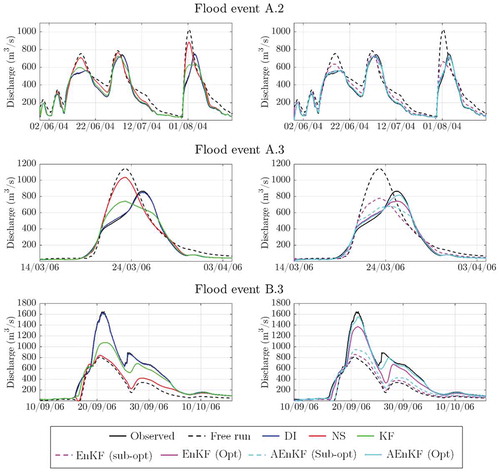
It is interesting to note that the results from KF and EnKF differ based on the approach (sub-optimal or optimal) used to estimate the model error variance S. The results show that model error estimation in Kalman filtering approaches can significantly affect the DA performance. The reasons for such incongruence can be found in the fact that fixing the ensemble spread in the sub-optimal EnKF to the same value of the process noise in KF does not guarantee the optimal use of EnKF. In fact, the small value of the covariance S results in a small spread in the EnKF and in its consequent sub-optimal use. Such low spread of the model ensemble indicates that the EnKF trusts the model more than the assimilated observations, with a consequent low model performance.

The Optimal EnKF tends to outperform both KF and the sub-optimal EnKF. The AEnKF approach with W = 2 produced results comparable with DI. This means that augmenting past observations can improve model performance even in cases of a sub-optimal filter. A way to solve this issue is to optimally estimate the ensemble spread, as described in Section 4. It can be observed that optimal EnKF and AEnKF outperform the sub-optimal approaches and KF. The optimal AEnKF shows performance similar to DI.

Table 6 presents NSE and Bias values for reaches A and B for the six different flood events at the analysis time (i.e. lead time = 0 h). As expected, the lowest values of NSE are obtained without any model update. The best model improvements, in terms of both NSE and Bias, are achieved with DI and optimal AEnKF, due to the high auto- and cross-correlation of streamflow, while NS and sub-optimal EnKF produce less satisfactory model results. Overall, streamflow in Reach A is overestimated (Bias > 1), while opposite results are obtained in Reach B.1 and B.2 (Bias < 1). This can be due to an inefficient calibration of the parameter K₃: (Equation (5)), which represents lateral inflow along the river reach. High auto- and cross-correlation of observations for short lag times (Fig. 2) may affect performance at the analysis time step, although additional analysis is left as a future endeavour.

Table 6. Deterministic (NSE and Bias) and probabilistic (CRPS and BSS) performance measures obtained in Experiment 1.

Event	Index	NoDA	DI	NS	KF	EnKF (Sub-opt)	EnKF (Opt)	AEnKF (Sub-opt)	AEnKF (Opt)
A.1	NSE	0.15	1.00	0.69	0.92	0.82	0.99	0.91	0.99
	Bias	1.33	1.01	1.10	1.03	1.05	1.02	1.00	1.01
	CRPS	143.10	4.85	78.53	33.70	57.43	11.43	23.37	8.50
	BSS	-	-	-	-	−0.33	0.83	0.60	0.89
A.2	NSE	0.69	1.00	0.85	0.97	0.93	1.00	0.99	1.00
	Bias	1.23	1.01	1.09	1.03	1.08	1.02	1.02	1.01
	CRPS	89.94	3.02	49.92	21.78	41.38	8.00	10.93	5.71
	BSS	-	-	-	-	0.09	0.92	0.86	0.95
A.3	NSE	0.50	1.00	0.63	0.90	0.83	0.98	0.94	1.00
	Bias	1.24	1.01	1.14	1.03	1.00	0.99	0.97	1.00
	CRPS	115.28	4.96	87.30	45.94	68.04	16.11	33.66	7.89
	BSS	-	-	-	-	−0.88	0.63	−0.11	0.91
B.1	NSE	0.90	1.00	0.93	0.97	0.92	0.99	0.93	0.99
	Bias	0.99	1.00	0.99	0.99	0.98	0.99	0.96	1.00
	CRPS	77.15	8.99	61.00	30.59	62.75	20.23	37.98	11.84
	BSS	-	-	-	-	0.42	0.80	0.54	0.87
B.2	NSE	0.95	1.00	0.97	0.99	0.98	1.00	0.99	1.00
	Bias	1.11	1.00	1.07	1.02	1.07	1.02	1.01	1.01
	CRPS	107.95	15.08	82.37	38.86	72.28	16.26	20.93	13.50
	BSS	-	-	-	-	0.14	0.80	0.82	0.82
B.3	NSE	0.45	1.00	0.56	0.86	0.54	0.91	0.66	0.99
	Bias	0.50	0.99	0.61	0.83	0.55	0.84	0.62	0.95
	CRPS	230.01	6.30	180.43	85.08	205.53	70.42	172.70	23.20
	BSS	-	-	-	-	−0.11	0.84	−0.11	0.95

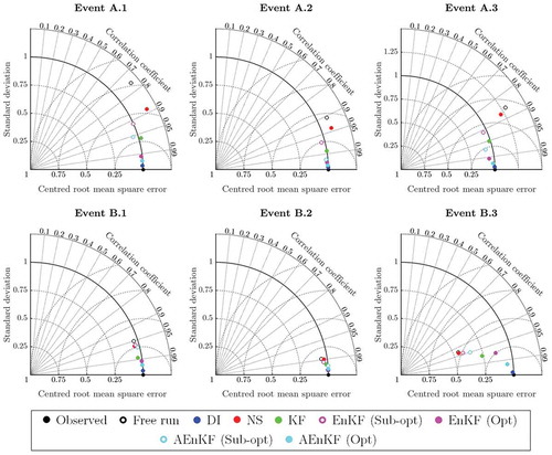
Figure 5 presents Taylor diagrams for reaches A and B for the six flood events at the analysis time. Taylor diagrams graphically summarize similarities between simulations and observations with root mean square deviation (RMSD), correlation and standard deviation between observations and simulations. This means that the closest the simulation result, for a given DA method, is to the observations (black point) in the Taylor diagram, the better. High correlation values are achieved using DI and optimal ensemble methods. On the other hand, the NS method does not allow us to significantly improve model performance if compared with results without update. In Table 6 the probabilistic measures CRPS and BSS are reported. As expected, values of BSS close to 1 are achieved for optimal AEnKF, with the highest values for flood events A.2 and B.3. Similarly, small CRPS values are obtained for DI and optimal AEnKF.

Figure 5. Taylor diagrams obtained for reaches A and B using different DA methods (lumped routing).

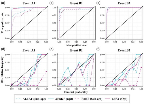
Figure 6 presents the ROC curve and the reliability diagram for reaches A and B for three different flood events (for lead time 1 hour) that occurred in the analysed time period. In Figure 6, the optimal models EnKF (Opt) and AEnKF (Opt) provide the highest reliability and the highest discrimination ability with respect to the sub-optimal models (Sub-opt). This is particularly true in the analysis of flood event A.1. Here, the optimal models experience an increase of 10% (AEnKF) and 16% (EnKF) in the value of the AUC indicator with respect to the sub-optimal models. The same can be said about BSS: the optimal models perform better than the sub-optimal ones, with a 66% (AEnKF) and 85% (EnKF) decrease in BSS from sub-optimal to optimal (see Table 6). In general, it is possible to consider the performance of the two optimal models as comparable, with the AEnKF marginally outperforming the EnKF, while EnKF (Sub-opt) is the best solution in all the analysed scenarios.

Figure 6. ROC (a, b, c) and reliability diagrams (d, e, f) for three selected flood events in reaches A and B.

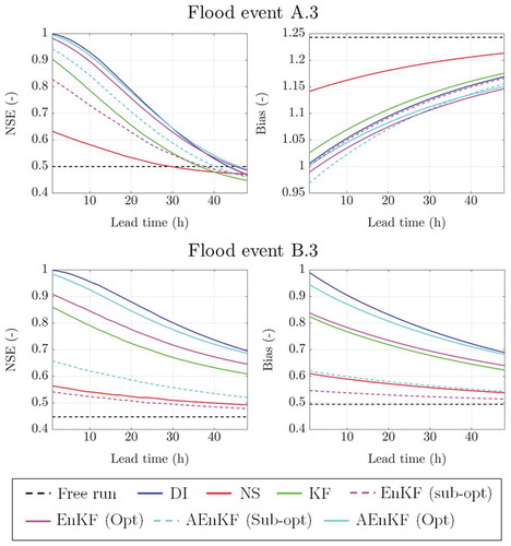
Figure 7 shows NSE and Bias as a function of lead time for flood events A.3 and B.3. Observations at the upstream stations are used as perfect forecasts for this analysis. As previously, DI produces the largest improvement in streamflow over a range of lead times for both flood events. AEnKF and KF also noticeably improve streamflow results. However, for flood event A.3, NS tends to give comparable NSE values to those obtained using the other DA methods used in this study for high lead times. In Figure 7, gains of updating by DA methods last longer in Reach B (lower panel) compared to Reach A (upper panel), which indicates that the performance of DA may be affected by characteristics of river observations, such as auto- and cross-correlation (Fig. 2).

Figure 7. Comparison of NSE and Bias as a function lead time among the different DA methods for flood events A.3 and B.3 (lumped routing).

4.2 Experiment 2

Lumped and distributed 3-par Musk model structures were used to estimate streamflow values along the Trinity River flowing from Fort Worth to the urbanized area of Dallas. For AEnKF, when W > 5, any additional past observations provided negligible model updates.

Streamflow observations recorded at two sensor locations – Grand Prairé (GPRT2) and Dallas (DALT2) – during the flood events of May–August 2015 in the DFW area are assimilated. In particular, three different scenarios of assimilation of streamflow observations by location were introduced for the distributed structure: (a) at the GPRT2 sensor; (b) at the DALT2 sensor; and (c) from both GPRT2 and DALT2 sensors. However, for the lumped structure, only observations at DALT2 were integrated within the model. Simulated streamflow values were compared to the observed ones at DALT2 because of the strategic position of this flow sensor in flood risk management for the DFW area.

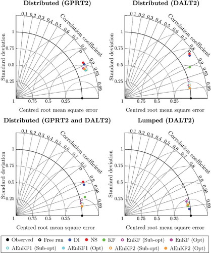
The results presented in Figure 8 and Table 7 show an overestimation of the observed flow at the DALT2 station. The Taylor diagrams for the distributed model show that, as expected, lower standard deviations and RMSD are achieved for assimilation at both GPRT2 and DALT2. In particular, good model improvements are obtained with the sensor at DALT2, while the opposite results can be seen for assimilation only at GPRT2. This suggests that additional sensors close to the Dallas area would further improve the model results, and may help reduce flood risk. High correlation values are achieved for assimilation in both distributed and lumped model structures. The DI provides the best model improvement for the Dallas station with the lumped model. Optimal and sub-optimal ensemble DA methods tend to outperform KF in all three scenarios of assimilation locations for the distributed model, while DI provides poor model performance.

Table 7. Deterministic (NSE and Bias) and probabilistic (CRPS and BSS) performance measures obtained in Experiment 2.

Method	Lumped				Distributed
	NSE	Bias	CRPS	BSS	NSE	Bias	CRPS	BSS
NoDA	0.77	0.96	77.04	-	0.47	1.11	139.52	-
DI	0.99	0.99	16.01	-	0.56	1.10	127.15	-
NS	0.98	0.99	22.37	-	0.52	1.11	130.87	-
KF	0.98	0.99	21.36	-	0.77	1.07	89.21	-
EnKF (Sub-Opt)	0.94	0.97	29.31	0.60	0.93	1.00	30.74	0.49
EnKF (Opt)	0.95	0.96	27.55	0.67	0.96	0.99	22.79	0.70
AEnKF1 (Sub-Opt)	0.96	0.97	23.56	0.66	0.95	1.00	24.44	0.61
AEnKF1 (Opt)	0.96	0.97	22.51	0.71	0.97	0.99	19.31	0.74
AEnKF2 (Sub-Opt)	0.96	0.98	21.46	0.68	0.96	1.00	21.14	0.66
AEnKF2 (Opt)	0.97	0.97	20.62	0.72	0.98	0.99	17.18	0.77

Figure 8. Taylor diagrams obtained using different DA methods for different locations of the flow sensors (distributed routing).

The values of NSE and Bias, obtained for the different model structures, are reported in Table 7. High NSE values were obtained for AEnKF with W = 5, followed by AEnKF with W = 2 in the distributed model. The DI gave high NSE values because local updates were only at the assimilation point and not along the entire river reach for the lumped model structure. However, comparison between the NSE values shows different results from using KF, sub-optimal EnKF and optimal EnKF, highlighting that Kalman filtering methods are very sensitive to the proper model error estimation. Overall, for the distributed model, the streamflow at DALT2 tends to be overestimated (Bias > 1). The frequent overestimation of the observed flow may be due to inefficient calibration of the parameter K₃ (Equation (5)).

Figure 9 shows the streamflow profile along sub-reach C1 obtained for assimilation at station GPRT2 and at two different time steps. As previously discussed, assimilation using both DI and NS does not affect the profile upstream of the assimilation point. Different results were obtained for Kalman filter methods. In the KF-based methods (KF, sub-optimal EnKF and sub-optimal AEnKF), all the model states were updated as a response to assimilation at a single location. This is due to the distributed nature of the Kalman gain matrix K. In fact, as shown in Section 5, the maximum value of K is achieved at the assimilation point, while the value of K reduces proportionally to the distance from the assimilation point. Another interesting aspect is that, in the case of KF, a discontinuity in the profile can be observed at the assimilation point. However, such a discontinuity is not present in the ensemble methods.

Figure 9. Streamflow profile and storage along sub-reach C1 at two particular time steps for assimilation in GPRT2 (distributed routing).

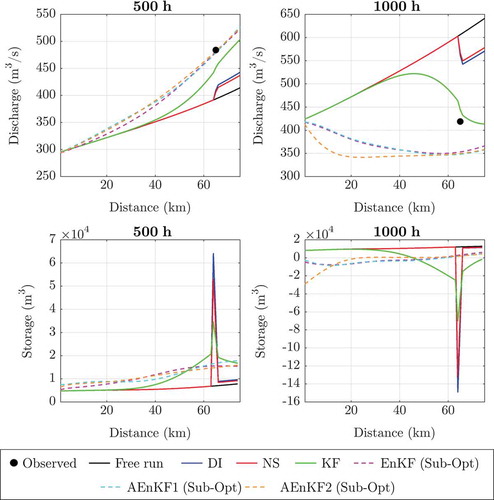
The same behaviour can be observed in Figure 9, where the water storage (m³) between one cross-section and the one upstream is calculated along sub-reach C1 for the same time steps. It can be observed that DI, NS and KF induce an abrupt change in the water storage at the sensor location, while in ensemble methods a smooth variation of storage is observed along the river. However, it is interesting to observe in Figure 9 that, in ensemble methods, the state update at upstream locations induces a non-univocal profile in both EnKF and AEnKF. This is due to the ensemble generation at the boundary conditions, which generates different ensemble trajectories at upstream locations.

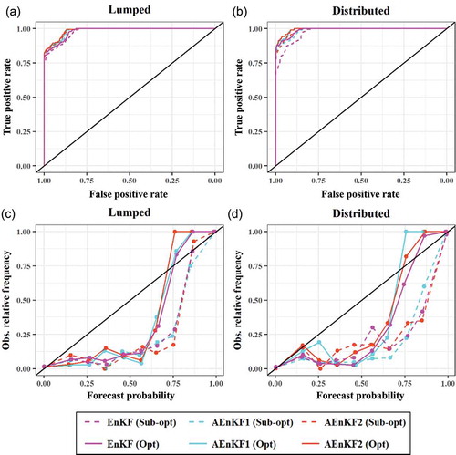
Figure 10 shows the ROC curve and reliability diagram for the probabilistic analysis of the lumped and distributed modes. By analysing the plot and observing the statistical indicators, it is evident that all the models provide excellent reliability (BSS in the range [0.23; 0.37]) and discrimination ability score (AUC always > 0.98). In general, the distributed optimal models can be considered as the best alternative, having performances that are marginally better than the lumped non-optimal models. However, this performance improvement can be considered as marginal in most cases. Once again, EnKF (Sub-opt) can be considered a better solution than the rest.

Figure 10. ROC (a and b) and reliability diagrams (c and d) for the flood event on Reach C for lumped and distributed structures A and B.

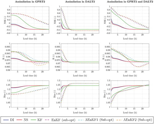
In Figure 11, the NSE, R and Bias values of model prediction, for up to 24 h lead time, are shown for the June 2015 flood event, in Reach C (Peak 1 in Figure 3), where the model simulation overestimated the observed streamflow hydrograph. It can be seen that assimilation at DALT2 station provides an overall improvement in the model predictions. However, such improvement is lost after a few hours, leading to NSE, R and Bias values equal to those obtained without any model update. Besides, assimilation at GPRT2 station gives higher values of the statistical indexes for high lead times. This is due to the propagation effect from the assimilation point up to the target point at DALT2. As described above, AEnKF and EnKF provide better model performance for any lead time values, while DI and NS are the less effective and accurate DA methods for the distributed model in all scenarios and sensor locations. In Table 8 we summarize the advantages and disadvantages of the different DA methods, in terms of updating the 3-par Musk model.

Table 8. Summary of the advantages and disadvantages of the five DA methods, in terms of updating the 3-par Musk model used in this study.

	Advantages	Disadvantages
DI	Best performance in cases of lumped modelling	Assimilation effects dissipate quickly in cases of distributed modelling
NS	Easy to implement	Poor model performance in both lumped and distributed model structures
KF	Good in cases of linear model Overall good results in both model structures	Sensitive to model error estimation
EnKF	Good results in cases of distributed model structure Good performance for optimal model error estimation	Sensitive to ensemble spread definition Poor results in cases of lumped model structure for sub-optimal model error estimation Computationally expensive Uncertain representation of flow profile in cases of distributed modelling
AEnKF	Best performance in cases of both lumped and distributed modelling Better results with the increasing number of past observations	Sensitive to ensemble spread definition Computationally most expensive Uncertain representation of flow profile in cases of distributed modelling

Figure 11. Comparison of observations and model predictions, in terms of NSE, R and Bias, for different lead times and different flow sensor locations during Peak 1 in the June 2015 flood event (distributed routing).

5 Conclusions

In this study, we evaluated the effects of different DA approaches – direct insertion (DI), nudging scheme (NS), Kalman filter (KF), ensemble Kalman filter (EnKF) and asynchronous ensemble Kalman filter (AEnKF) – on the assimilation of streamflow observations from within two structures, lumped and distributed, of a three-parameter Muskingum (3p-Musk) model. Sub-optimal and optimal methods were used to estimate the ensemble spread for EnKF and AEnKF approaches.

This study shows that, for the specific case studies, assimilation of streamflow observations increases the performance of the hydrological routing model. Overall, higher statistical performance is obtained with a lumped model compared to a distributed model. This is because, in distributed modelling, the maximum update is carried out at the assimilation location, while at the other point the adjustment via updating is relatively small. In the case of a lumped model, the entire river reach receives the same amount of update, with a consequent higher model improvement at the downstream target point. In addition, using past observations to update model states (e.g. the AEnKF method) helps to achieve satisfactory model results even with sub-optimal ensemble spread.

The results obtained in Experiment 1 (reaches A and B) show that DI provided the best improvement among the five DA methods used due to the model structure (only one model state) and the assumption on perfect flow observations. Comparably good results were achieved for the optimal EnKF and AEnKF approaches. Sub-optimal AEnKF performed better than KF and sub-optimal EnKF, achieving similar results to DI. Kalman filtering approaches were noticeably sensitive to the definition of model error. Assimilation of streamflow observations using NS produced unsatisfactory model improvements.

For Experiment 2 and the distributed model of Reach C, the best model improvement was obtained by assimilating flow observations at distributed upstream and downstream sensors. In contrast, assimilation only at the upstream station resulted in small improvement. Among all the DA methods, the highest model performance was achieved using optimal and sub-optimal AEnKF with W = 5 in both analysis and forecasting steps. Additional inclusion of past observations longer than 5 hours didn’t increase the model performance in the AEnKF approach. For the lumped structure of Reach C, DI provided the best model performance, as for reaches A and B. However, for the distributed structure, DI was not as effective as for the lumped structure in Reach C. This is mainly because DI affects the model states only at that particular location and downstream of it, while upstream of the assimilation point is not changed due to the nature of the Muskingum model. An abrupt change in the flow water storage profile was observed in the upstream direction from the assimilation point when using DI, NS and KF, while a smooth variation of flow was observed in ensemble methods.

It is expected that these results will serve as possible guidelines for selection of assimilation methods and model structures for improved early warning systems in assimilating increasingly abundant real-time observations into linear hydrological routing models. Suggestions for future research include model error specification considering the spatial and temporal correlation, and comparison between AEnKF and variational data assimilation which implement asynchronous assimilation in different approaches.

Acknowledgements

We would like to thank the West Gulf River Forecast Center for providing river discharge data.

Disclosure statement

No potential conflict of interest was reported by the authors.

Additional information

Funding

This research was funded in the framework of the European FP7 Project WeSenseIt: Citizen Observatory of Water [grant agreement no. 308429]. Support for Seongjin Noh and Dong-Jun Seo was provided by the National Science Foundation under Grant CyberSEES-1442735 (Dong-Jun Seo, University of Texas at Arlington, PI), and by NOAA/OAR/OWAQ/JTTI under Grant NA17OAR4590174. This support is gratefully acknowledged; Directorate for Computer and Information Science and Engineering [CyberSEES-1442735]; Seventh Framework Programme [308429].

References

- Abaza, M., et al., 2014. Sequential streamflow assimilation for short-term hydrological ensemble forecasting. Journal of Hydrology, 519, 2692–2706. doi:10.1016/j.jhydrol.2014.08.038
- Abaza, M., Garneau, C., and Anctil, F., 2015. Comparison of sequential and variational streamflow assimilation techniques for short-term hydrological forecasting. Journal of Hydrologic Engineering, 20 (2). doi:10.1061/(ASCE)HE.1943-5584.0001013
- Anderson, J.L., 2001. An ensemble adjustment Kalman filter for data assimilation. Monthly Weather Review, 129, 2884–2903. doi:10.1175/1520-0493(2001)129<2884:AEAKFF>2.0.CO;2
- Andreadis, K.M., et al., 2007. Prospects for river discharge and depth estimation through assimilation of swath-altimetry into a raster-based hydrodynamics model. Geophysical Research Letters, 34 (10). doi:10.1029/2007GL029721
- Andreadis, K.M. and Lettenmaier, D.P., 2006. Assimilating remotely sensed snow observations into a macroscale hydrology model. Advances in Water Resources, 29 (6), 872–886. doi:10.1016/j.advwatres.2005.08.004
- Andreadis, K.M. and Schumann, G.J.-P., 2014. Estimating the impact of satellite observations on the predictability of large-scale hydraulic models. Advances in Water Resources, 73, 44–54. doi:10.1016/j.advwatres.2014.06.006
- Barbetta, S., et al., 2011. Case study: improving real-time stage forecasting Muskingum model by incorporating the rating curve model. Journal of Hydrologic Engineering, 16 (6), 540–557. doi:10.1061/(ASCE)HE.1943-5584.0000345
- Barth, B., Ringen, S., and Sallas, J., 2014. City of Dallas Floodway System (DFS) case study: 100-year levee remediation. In: Rocky Mountain Geo-Conference 2014. Reston, VA: American Society of Civil Engineers, 59–68. doi:10.1061/9780784413807.004
- Barthelemy, S., et al., 2017. Ensemble-based data assimilation for operational flood forecasting - On the merits of state estimation for 1-D hydrodynamic forecasting through the example of the “Adour maritime” river. Journal of Hydrology, 552, 210–224. doi:10.1016/j.jhydrol.2017.06.017
- Beven, K., 2016. Facets of uncertainty: epistemic uncertainty, non-stationarity, likelihood, hypothesis testing, and communication. Hydrological Sciences Journal, 61, 1652–1665. doi:10.1080/02626667.2015.1031761
- Biancamaria, S., et al., 2011. Assimilation of virtual wide swath altimetry to improve Arctic river modeling. Remote Sensing of Environment, 115, 373–381. doi:10.1016/j.rse.2010.09.008
- Boku, L. and Xuewei, Q., 1987. Some problems with the Muskingum method. Hydrological Sciences Journal, 32, 485–496. doi:10.1080/02626668709491207
- Brocca, L., et al., 2010. Improving runoff prediction through the assimilation of the ASCAT soil moisture product. Hydrology and Earth System Sciences, 14, 1881–1893. doi:10.5194/hess-14-1881-2010
- Brocca, L., et al., 2012. Assimilation of surface- and root-zone ASCAT soil moisture products into rainfall-runoff modeling. IEEE Transactions on Geoscience and Remote Sensing, 50 (7 PART1), 2542–2555. doi:10.1109/TGRS.2011.2177468
- Brochero, D., Anctil, F., and Gagné, C., 2011. Simplifying a hydrological ensemble prediction system with a backward greedy selection of members – part 1: optimization criteria. Hydrology and Earth System Sciences, 15, 3307–3325. doi:10.5194/hess-15-3307-2011
- Bröcker, J., 2012. Evaluating raw ensembles with the continuous ranked probability score. Quarterly Journal of Royal Meteorological Society, 138, 1611–1617. doi: 10.1002/qj.1891
- Clark, M.P., et al., 2008. Hydrological data assimilation with the ensemble Kalman filter: use of streamflow observations to update states in a distributed hydrological model. Advances in Water Resources, 31, 1309–1324. doi:10.1016/j.advwatres.2008.06.005
- Daley, R., 1991. Atmospheric data analysis. Cambridge, UK: Cambridge University Press, Cambridge Atmospheric and Space Science Series.
- Deb, K., et al., 2002. A fast and elitist multiobjective genetic algorithm: NSGA-II. IEEE Transactions on Evolutionary Computation, 6, 182–197. doi:10.1109/4235.996017
- DeChant, C.M. and Moradkhani, H., 2012. Examining the effectiveness and robustness of data assimilation methods for calibration and quantification of uncertainty in hydrologic forecasting. Water Resources Research, 48, W04518. doi:10.1029/2011WR011011
- Dee, D.P., 1995. On-line estimation of error covariance parameters for atmospheric data assimilation. Monthly Weather Review, 123(4), 1128–1145. doi:10.1175/1520-0493(1995)123<128:oleoec>2.0.CO;2
- Earl, R.A. and Vaughan, J.W., 2015. Asymmetrical response to flood hazards in south central Texas. Papers in Applied Geography, 1, 404–412. doi:10.1080/23754931.2015.1095792
- Evensen, G., 2003. The ensemble Kalman filter: theoretical formulation and practical implementation. Ocean Dynamics, 53, 343–367. doi:10.1007/s10236-003-0036-9
- Evensen, G., 2009. Data assimilation: the ensemble Kalman filter. 2nd ed. Berlin: Springer.
- Franz, K.J. and Hogue, T.S., 2011. Evaluating uncertainty estimates in hydrologic models: borrowing measures from the forecast verification community. Hydrology and Earth System Sciences, 15, 3367–3382. doi:10.5194/hess-15-3367-2011
- García-Pintado, J., et al., 2013. Scheduling satellite-based SAR acquisition for sequential assimilation of water level observations into flood modelling. Journal of Hydrology, 495, 252–266. doi:10.1016/j.jhydrol.2013.03.050
- Georgakakos, A.P., Georgakakos, K.P., and Baltas, E.A., 1990. A state-space model for hydrologic river routing. Water Resources Research, 26, 827–838. doi:10.1029/WR026i005p00827
- Giustarini, L., et al., 2011. Assimilating SAR-derived water level data into a hydraulic model: a case study. Hydrology and Earth System Sciences, 15, 2349–2365. doi:10.5194/hess-15-2349-2011
- Gochis, D.J., Yu, W., and Yates, D.N., 2015. The WRF-Hydro model technical description and user’s guide, version 3.0. NCAR Technical Document; p. 123. [accessed 2018 Jan 2]. http://www.ral.ucar.edu/projects/wrf_hydro/.
- Haddad, O.B., et al., 2015. Application of a hybrid optimization method in Muskingum parameter estimation. Journal of Irrigation and Drainage Engineering, 141, 4015026. doi:10.1061/(ASCE)IR.1943-4774.0000929
- Hajian-Tilaki, K., 2013. Receiver Operating Characteristic (ROC) curve analysis for medical diagnostic test evaluation. Caspian Journal of Internal Medicine, 4 (2), 627–635.
- Jean-Baptiste, N., et al., 2011. Data assimilation for real-time estimation of hydraulic states and unmeasured perturbations in a 1D hydrodynamic model. In: eds, B. Amaziane and D. Barrera. Mathematics and Computers in Simulation, MAMERN 2009: 3rd International Conference on Approximation Methods and Numerical Modeling in Environment and Natural Resources. Amsterdam: Elsevier, Vol. 81, 2201–2214. doi:10.1016/j.matcom.2010.12.021
- Kalman, R.E., 1960. A new approach to linear filtering and prediction problems. Journal of Basic Engineering, 82, 35–45. doi:10.1115/1.3662552
- Kim, Y., et al., 2013a. Estimating the 2011 largest flood discharge at the Kumano River using the 2d dynamic wave model and particle filters. Journal of Japan Society of Civil Engineers, Series B1 (Hydraulic Engineering), 69 (4), 163–168. doi:10.2208/jscejhe.69.I_163
- Kim, Y., et al., 2013b. Simultaneous estimation of inflow and channel roughness using 2D hydraulic model and particle filters. Journal of Flood Risk Management, 6, 112–123. doi:10.1111/j.1753-318X.2012.01164.x
- Kitanidis, P.K., and Bras, R. L., 1980. Real-time forecasting with a conceptual hydrologic model: 1. analysis of uncertainty. Water Resources Research, 16 (6), 1025–1033. doi:10.1029/WR016i006p01025
- Lahoz, W.A., and Schneider, P., 2014. Data assimilation: making sense of Earth Observation. Frontiers In Environmental Science. 2. doi:10.3389/fenvs.2014.00016
- Lee, H., et al., 2011. Variational assimilation of streamflow into three-parameter Muskingum routing model for improved operational river flow forecasting. In: The EGU General Assembly. Munich: EGU.
- Liu, Y., et al., 2008. Ensemble data assimilation for channel flow routing to improve operational hydrologic forecasting. In: The AGU Fall Meeting. Washington, DC: AGU.
- Liu, Y., et al., 2012. Advancing data assimilation in operational hydrologic forecasting: progresses, challenges, and emerging opportunities. Hydrology and Earth System Sciences, 16, 3863–3887. doi:10.5194/hess-16-3863-2012
- Liu, Y. and Gupta, H.V., 2007. Uncertainty in hydrologic modeling: toward an integrated data assimilation framework. Water Resources Research, 43, 1–18. doi:10.1029/2006WR005756
- Madsen, H., et al., 2003. Data assimilation in the MIKE 11 Flood Forecasting system using Kalman filtering. In: G. Blöschl, ed. Water Resources Systems— hydrological Risk, Management and Development (Proceedings of symposium IlS02b held during IUGG2003 al Sapporo. July 2003). Wallingford, UK: International Association of Hydrological Sciences, IAHS Publ. no. 281, 75–81.
- Madsen, H. and Skotner, C., 2005. Adaptive state updating in real-time river flow forecasting - A combined filtering and error forecasting procedure. Journal of Hydrology, 308, 302–312. doi:10.1016/j.jhydrol.2004.10.030
- Matgen, P., et al., 2010. Towards the sequential assimilation of SAR-derived water stages into hydraulic models using the Particle Filter: proof of concept. Hydrology and Earth System Sciences, 14, 1773–1785. doi:10.5194/hess-14-1773-2010
- Maybeck, P.S., 1982. Stochastic models, estimation, and control. New York, NY: Academic Press.
- Mazzoleni, M., 2017. Improving flood prediction assimilating uncertain crowdsourced data into hydrological and hydraulic models. Thesis (PhD). UNESCO-IHE PhD Thesis Series, CRC Press, Leiden, The Netherlands.
- McCarthy, G.T., 1938. The unit hydrograph and flood routing. Unp ublished manuscript presented at a conference of the North Atlantic Division. US Army, Corps of Engineers, 24 June 1938.
- McLaughlin, D., 1995. Recent developments in hydrologic data assimilation. Reviews of Geophysics, 33, 977–984. doi:10.1029/95RG00740
- McLaughlin, D., 2002. An integrated approach to hydrologic data assimilation: interpolation, smoothing, and filtering. Advances in Water Resources, 25, 1275–1286. doi:10.1016/S0309-1708(02)00055-6
- Moradkhani, H., et al., 2005a. Uncertainty assessment of hydrologic model states and parameters: sequential data assimilation using the particle filter. Water Resources Research, 41, W05012. doi:10.1029/2004WR003604
- Moradkhani, H., et al., 2005b. Dual state-parameter estimation of hydrological models using ensemble Kalman filter. Advances in Water Resources, 28 (2), 135–147. doi:10.1016/j.advwatres.2004.09.002
- Moradkhani, H., DeChant, C.M., and Sorooshian, S., 2012. Evolution of ensemble data assimilation for uncertainty quantification using the particle filter-Markov chain Monte Carlo method. Water Resources Research, 48, W12520. doi:10.1029/2012WR012144
- Murphy, A.H. and Winkler, R.L., 1987. A general framework for forecast verification. Monthly Weather Review, 115, 1330–1338. doi:10.1175/1520-0493(1987)115<1330:AGFFFV>2.0.CO;2
- Nash, J.E. and Sutcliffe, J.V., 1970. River flow forecasting through conceptual models part I — A discussion of principles. Journal of Hydrology, 10, 282–290. doi:10.1016/0022-1694(70)90255-6
- Neal, J., et al., 2009. A data assimilation approach to discharge estimation from space. Hydrological Processes, 23, 3641–3649. doi:10.1002/hyp.7518
- Neal, J.C., Atkinson, P.M., and Hutton, C.W., 2007. Flood inundation model updating using an ensemble Kalman filter and spatially distributed measurements. Journal of Hydrology, 336, 401–415. doi:10.1016/j.jhydrol.2007.01.012
- Neal, J.C., Atkinson, P.M., and Hutton, C.W., 2012. Adaptive space–time sampling with wireless sensor nodes for flood forecasting. Journal of Hydrology, 414–415, 136–147. doi:10.1016/j.jhydrol.2011.10.021
- Noh, S.J., et al., 2013. Ensemble Kalman filtering and particle filtering in a lag-time window for short-term streamflow forecasting with a distributed hydrologic model. Journal of Hydrologic. Engineering, 18, 1684–1696. doi:10.1061/(ASCE)HE.1943-5584.0000751
- O’Donnell, T., 1985. A direct three-parameter Muskingum procedure incorporating lateral inflow. Hydrological Sciences Journal, 30, 479–496. doi:10.1080/02626668509491013
- Park, S.K. and Xu, L., 2013. Data assimilation for atmospheric, oceanic and hydrologic applications. Berlin: Springer Science & Business Media.
- Pauwels, V.R.N. and De Lannoy, G.J.M., 2006. Improvement of modeled soil wetness conditions and turbulent fluxes through the assimilation of observed discharge. Journal of Hydrometeorology, 7 (3), 458–477. doi:10.1175/JHM490.1
- Pauwels, V.R.N. and De Lannoy, G.J.M., 2009. Ensemble-based assimilation of discharge into rainfall-runoff models: A comparison of approaches to mapping observational information to state space. Water Resources Research, 45 (8), W08428. doi:10.1029/2008WR007590
- Phillips, J.D., 2008. Geomorphic controls and transition zones in the lower Sabine River. Hydrological Processes, 22, 2424–2437. doi:10.1002/hyp.6835
- Press, W.H., et al., 1992. Numerical recipes in FORTRAN. 2nd ed. Cambridge, UK: Cambridge University Press.
- Puente, C.E. and Bras, R.L., 1987. Application of nonlinear filtering in the real time forecasting of river flows. Water Resources Research, 23, 675–682. doi:10.1029/WR023i004p00675
- Rakovec, O., et al., 2012. State updating of a distributed hydrological model with ensemble Kalman filtering: effects of updating frequency and observation network density on forecast accuracy. Hydrology and Earth System Sciences, 16, 3435–3449. doi:10.5194/hess-16-3435-2012
- Rakovec, O., et al., 2015. Operational aspects of asynchronous filtering for flood forecasting. Hydrology and Earth System Sciences, 19, 2911–2924. doi:10.5194/hess-19-2911-2015
- Rakovec, O., et al., 2016. Improving the realism of hydrologic model functioning through multivariate parameter estimation. Water Resources Research, 52, 7779–7792. doi:10.1002/2016WR019430
- Refsgaard, J.C., 1997. Validation and intercomparison of different updating procedures for real-time forecasting. Nordic Hydrology, 28, 65–84. doi:10.2166/nh.1997.005
- Reichle, R., McLaughlin, D.B., and Entekhabi, D., 2002. Hydrologic data assimilation with the ensemble Kalman filter. American Meteorological Society, 130, 103–114. doi:10.1175/1520-0493(2002)130<0103:HDAWTE>2.0.CO;2
- Reichle, R.H., Crow, W.T., and Keppenne, C.L., 2008. An adaptive ensemble Kalman filter for soil moisture data assimilation. Water Resources Research, 44, W03423. doi:10.1029/2007WR006357
- Ricci, S., et al., 2011. Correction of upstream flow and hydraulic state with data assimilation in the context of flood forecasting. Hydrology and Earth System Sciences, 15, 3555–3575. doi:10.5194/hess-15-3555-2011
- Richardson, D.S., 2001. Measures of skill and value of ensemble prediction systems, their interrelationship and the effect of ensemble size. Quarterly Journal of the Royal Meteorological Society, 127, 2473–2489. doi:10.1002/qj.49712757715
- Sakov, P., Evensen, G., and Bertino, L., 2010. Asynchronous data assimilation with the EnKF. Tellus A, 62, 24–29. doi:10.1111/j.1600-0870.2009.00417.x
- Samani, H.M.V. and Jebelifard, S., 2003. Design of circular urban storm sewer systems using multilinear Muskingum flow routing method. Journal of Hydraulic Engineering, 129, 832–838. doi:10.1061/(ASCE)0733-9429(2003)129:11(832)
- Schumann, G.J.-P., et al., 2016. Unlocking the full potential of Earth observation during the 2015 Texas flood disaster. Water Resources Research, 52, 3288–3293. doi:10.1002/2015WR018428
- Seo, D.-J., Koren, V., and Reed, S., 2003. Improving a priori estimates of hydraulic parameters in a distributed routing model via variational assimilation of long-term streamflow data. IAHS Publications Series (Red Books), 282, 138–414.
- Sun, L., et al., 2016. Review of the Kalman-type hydrological data assimilation. Hydrological Sciences Journal, 61 (13), 2348–2366. doi:10.1080/02626667.2015.1127376
- Todini, E., 2007. A mass conservative and water storage consistent variable parameter Muskingum-Cunge approach. Hydrology and Earth System Sciences, 11, 1645–1659. doi:10.5194/hess-11-1645-2007
- Trambauer, P., et al., 2015. Hydrological drought forecasting and skill assessment for the Limpopo River basin, southern Africa. Hydrology and Earth System Sciences, 19, 1695–1711. doi:10.5194/hess-19-1695-2015
- USGS (US Geological Survey), 2016. USGS discharge data for Riverside [WWW Document]. Available from: https://waterdata.usgs.gov/nwis/sw [Accessed 2 January 2018].
- Verlaan, M., 1998. Efficient Kalman filtering algorithms for hydrodynamic models. Thesis (PhD). Delft University of Technology, Delft, The Netherlands
- Walker, J.P. and Houser, P.R., 2005. Hydrologic data assimilation. In: J. Tiefenbacher, eds. Approaches to managing disaster – assessing Hazards, emergencies and disaster impacts. London: InTechOpen, 233–234. doi:10.5772/1112
- Walker, J.P., Willgoose, G.R., and Kalma, J.D., 2001. One-dimensional soil moisture profile retrieval by assimilation of near-surface observations: a comparison of retrieval algorithms. Advances in Water Resources, 24 (6), 631–650. doi:10.1016/S0309-1708(00)00043-9
- Weerts, A.H. and El Serafy, G.Y.H., 2006. Particle filtering and ensemble Kalman filtering for state updating with hydrological conceptual rainfall–runoff models. Water Resources Research, 42, 1–17. doi:10.1029/2005WR004093
- Weigel, A.P., Liniger, M.A., and Appenzeller, C., 2007. The discrete brier and ranked probability skill scores. Monthly Weather Review, 135, 118–124. doi:10.1175/MWR3280.1
- WMO (World Meteorological Organization), 1992. Simulated real-time intercomparison of hydrological models. Geneva, Switzerland: World Meteorological Organization, WMO Operational Hydrology Report.
- Xu, D.-M., Qiu, L., and Chen, S.-Y., 2012. Estimation of nonlinear Muskingum model parameter using differential evolution. Journal of Hydrologic Engineering, 17, 348–353. doi:10.1061/(ASCE)HE.1943-5584.0000432
- Yuan, X., et al., 2016. Parameter identification of nonlinear Muskingum model with backtracking search algorithm. Water Resources Management, 30, 2767–2783. doi:10.1007/s11269-016-1321-y