Regional flood frequency analysis using support vector regression in arid and semi-arid regions of Iran

ABSTRACT

Regional flood frequency analysis (RFFA) was carried out on data for 55 hydrometric stations in Namak Lake basin, Iran, for the period 1992–2012. Flood discharge of specific return periods was computed based on the log Pearson Type III distribution, selected as the best regional distribution. Independent variables, including physiographic, meteorological, geological and land-use variables, were derived and, using three strategies – gamma test (GT), GT plus classification and expert opinion – the best input combination was selected. To select the best technique for regionalization, support vector regression (SVR), adaptive neuro-fuzzy inference system (ANFIS), artificial neural network (ANN) and nonlinear regression (NLR) techniques were applied to predict peak flood discharge for 2-, 5-, 10-, 25-, 50- and 100-year return periods. The GT + ANFIS and GT + SVR models gave better performance than the ANN and NLR models in the RFFA. The results of the input variable selection showed that the GT technique improved the model performance.

KEYWORDS:

• regionalization
• support vector machine
• gamma test
• peak discharge

Editor R. Woods Associate editor E. Volpi

1 Introduction

Estimating accurate flood magnitudes for various return periods is essential for many hydrological and hydraulic engineering projects (Srinivas et al. 2008). Determining the design flood is also necessary for hydrological analysis and integrated flood control projects (Stedinger and Griffis 2008). Regional flood frequency analysis (RFFA) is used to transfer information on flood characteristics from gauged to ungauged watersheds (Blöschl and Sivapalan 1997, Pallard et al. 2009, Rahman et al. 2014). An RFFA usually involves data preparation, the identification of homogeneous regions, and development of regional estimation models (Dalrymple 1960, Jingyi and Hall 2004, Hosking and Wallis 2005, Rahman et al. 2014, Vafakhah and Eslamian 2014). To develop the regional flood prediction equations, commonly used techniques include the rational method, index flood method and quantile regression technique (QRT). Most of the above RFFA methods assume a linear relationship between flood statistics and predictor variables, generally in the log domain, when developing the regional prediction equations. However, most hydrological processes are nonlinear and exhibit a high degree of spatial and temporal variability; hence, a simple log transformation cannot guarantee achievement of linearity in modelling (Aziz et al. 2014).

In recent years, there has been increasing interest in the use of artificial neural network (ANN) and adaptive neuro-fuzzy inference system (ANFIS) techniques for modelling the stage–discharge relationship (Vafakhah and Kahneh 2016); daily and monthly discharge (Nayak et al. 2004, Kurtulus and Razack 2010, Vafakhah 2012); daily and monthly suspended sediment prediction (Kisi et al. 2008, Cobaner et al. 2009); rainfall–runoff prediction (Talei et al. 2010, Ghafari and Vafakhah 2012, Kisi et al. 2013); evaporation prediction (Kişi 2006, Dogan et al. 2010); flood forecasting (Chau et al. 2005, Chen et al. 2006); and regional analysis of flow duration curves (Bozchaloei and Vafakhah 2015).

Studies by Jingyi and Hall (2004), Shu and Burn (2004), Dawson et al. (2006), Shu and Ouarda (2007, 2008) and Aziz et al. (2014, 2015, 2017) show the importance of data-driven techniques such as ANN and ANFIS in RFFA. Jingyi and Hall (2004) compared four approaches, namely the geographical approach, Ward’s cluster method, the fuzzy c-means method and a Kohonen neural network, for the delineation of homogeneous regions using the index flood method via multiple linear regression analysis and ANN in the southeast of China. The results showed that the ANN model was superior to the regression model. Shu and Burn (2004) applied ANN in RFFA in the UK, and their results indicated that regional analysis based on ANN was better than a nonlinear regression (NLR) approach. Dawson et al. (2006) compared an ANN approach, an empirical model (as presented in the Flood Estimation Handbook, FEH) and a NLR approach to estimate the T-year flood and the median of the annual maximum flood (index flood) over the UK. The results showed that ANNs were the same as FEH models for estimating the index flood. The ANN was superior to NLR for predicting the T-year flood. Shu and Ouarda (2007) compared two canonical correlation analysis (CCA)-based ANN models including a single ANN model and an ensemble ANN model in RFFA at 151 gauged catchments located in Quebec Province, Canada. They concluded that the CCA-based ensemble ANN model was superior to the single ANN models. Shu and Ouarda (2008) used ANFIS, ANN and NLR techniques in RFFA, using the same dataset as Shu and Ouarda (2007), and found that the ANFIS approach had similar results to the ANN approach and was better than both NLR and NLR with regionalization. Seckin and Guven (2012) compared gene-expression programming (GEP), linear genetic programming (LGP) and logistic regression (LR) for estimating the peak flood discharges at 543 catchments across Turkey. They found that the GEP was superior to the LGP and LR methods. Alobaidi et al. (2015) applied a generalized ensemble-based ANN in RFFA using the same dataset as Shu and Ouarda (2007). Their model showed similar performance compared to the CCA-based ensemble ANN models.

Aziz et al. (2014) applied ANN-based RFFA methods on a database consisting of 452 gauged catchments in eastern Australia. They found that ANN-based RFFA models outperformed the traditional QRT. Aziz et al. (2015) optimized the ANN model using a genetic algorithm (GA) – GAANN – and compared it with the ANN model and traditional QRT in RFFA using the Aziz et al. (2014) dataset. The results showed that the ANN model was superior to the GAANN model, but both the GAANN and ANN methods outperformed the traditional QRT model. Again using the 2014 dataset, Aziz et al. (2017) compared the ANN model, GEP and traditional QRT in RFFA, and found that the ANN model was superior to GEP and both ANN and GEP methods outperformed the traditional QRT method.

The support vector machine (SVM) is one of the most widely used groups of data-driven techniques in hydrology (Dibike et al. 2001, Liong and Sivapragasam 2002, Bray and Han 2004, Asefa et al. 2006, Lin et al. 2006, Yu et al. 2006, Afiq et al. 2013). Gizaw and Gan (2016) compared support vector regression (SVR) and ANN models in RFFA for two study areas: southeastern British Columbia (26 catchments) and southern Ontario (23 catchments), Canada. The SVR model outperformed the ANN model for the two study areas.

The choice of catchment characteristics plays an important role in an RFFA (Rahman et al. 2014). One possible concern with an RFFA study is the multi-collinearity problem, because many catchment characteristics may be correlated. Multi-collinearity can be tested by variance inflation factor (VIF), principal component analysis (PCA), gamma test (GT) and stepwise regression (SR) (Kheirfam and Vafakhah 2015). The GT is a new method for selecting the best input combination and can determine the minimum number of data points required to build a good model (Kheirfam and Vafakhah 2015). Surveys such as that conducted by Moghaddamnia et al. (2009b) and Noori et al. (2011) showed that the GT technique improved the performance of ANN, ANFIS and SVM models. To our knowledge, no research has been done that surveyed SVR with three strategies for selecting the best input combination in RFFA. The primary aims of this study are: (1) to ascertain the effect of input variable selection using either GT, GT plus classification, or expert opinion-based selection on the performance of SVR, ANFIS, ANN and NLR models; and (2) to compare the SVR model with the ANFIS, ANN and NLR models in RFFA of the Namak Lake watershed, Iran.

2 Materials and methods

2.1 Study area and dataset

The Namak Lake watershed (watershed no. 41) (48°00′–53°00′E; 33°00′–36°00′N), with an area of 92 550 km², was selected as the study area. The mean catchment altitude varies between 800 and 4375 m a.s.l., with large variations within the watershed. The data for all the hydrometric stations in the Namak Lake watershed were obtained from the Iran Water Resources Research Company. The selected hydro-metric stations are distinguished by having a range of historical flood records of 20 years or longer, and the absence of hydraulic structures and direct water utilization from the river. For this study, 55 hydrometric stations with the same period of 20 years (1992–2012) were considered (Fig. 1). To complete the missing flood records, a regression equation was used between at-site flood peak discharge and maximum annual discharge.

2.2 Methodology

2.2.1 Calculation of flood peak discharge in various return periods

In order to compute flood peak discharge in various return periods for each hydrometric station, flood records were fitted, with the help of Easy Fit software, to seven probability distribution functions (pdfs): log Pearson Type III, three-parameter lognormal, two-parameter lognormal, Pearson Type III, Gumbel, normal and two-parameter gamma. The Kolmogorov-Smirnov (K-S) test was employed as a goodness-of-fit test. To determine the suitable regional pdf, an arbitrary ranking was used: the best fitted pdf was given a score of 1 and the worst a score of 7. Then, the sum of scores and the number of first-rank pdfs were computed for all 55 hydrometric stations. Finally, the suitable regional pdf was recognized. Flood discharge with 2-, 5-, 10-, 25-, 50- and 100-year return periods was estimated based on the suitable regional pdf (Ahn et al. 2014).

2.2.2 Derivation of data and features

At this stage, different variables including physiographical, meteorological, geological and land use in the upstream basins of the 55 hydrometric stations were derived. Catchment boundaries were extracted using ArcHydro extension based on the hydrometric station position and a digital elevation model (DEM) at a scale of 1:50 000 obtained from the Iran National Cartographic Centre. Physiographic characteristics of area, perimeter, drainage density, maximum height, minimum height, weighted average slope, average height, main stream length and main stream slope were extracted. To determine land use, a land-use map was derived using a 2002 land-use map, at a scale of 1:250 000, obtained from the Iran Forest, Ranges and Watershed Management Organization. The land-use map for each selected watershed was categorized into six types: water body, orchard, rangeland, irrigated farming, dryland farming and residential land, using Arc/GIS9.3 software. To determine impermeable formations, geological maps at a scale of 1:100 000 were obtained from the Iran Geological Survey and Mineral Exploration. Rock types (unconsolidated and consolidated) were derived using geological maps based on lithological categories. Meteorological characteristics: annual mean rainfall, annual mean evaporation, maximum 24-h rainfall and annual mean temperature, were obtained from the Iran Water Resources Research Company. Table 1 shows the descriptive statistics of watershed characteristics used in the study.

Table 1. Descriptive statistics of basin characteristics used in the study.

Variable	Definition	Unit	Statistical parameters
			Maximum	Minimum	Skewness	SD	Mean
Q2	Flood discharge with 2-year return period	m^3 s^−1	120.37	0.27	2.05	23.36	21.97
Q5	Flood discharge with 5-year return period	m^3 s^−1	191.53	0.77	1.26	41.66	44.75
Q10	Flood discharge with 10-year return period	m^3 s^−1	241.61	1.38	1.08	59.26	64.62
Q25	Flood discharge with 25-year return period	m^3 s^−1	392.6	2.7	1.38	94.3	96.88
Q50	Flood discharge with 50-year return period	m^3 s^−1	594.4	3.6	1.81	132.07	125.77
Q100	Flood discharge with 100-year return period	m^3 s^−1	837.66	4.16	2.08	190.69	165.64
A	Area	km^2	18 799.68	15.7	3.64	3908.41	1496.04
P	Perimeter	km	1260	20.96	2.97	266.86	188.99
Hmin	Minimum height	m a.s.l.^a	2248	815	−0.73	327.7	1639.11
Hmax	Maximum height	m a.s.l.	4323	2548	−0.1	506.68	3485.55
Hmean	Average height	m a.s.l.	3257.1	1305.32	−0.05	385.66	2296.54
DD	Drainage density	km km^−2	1.55	0.18	0.88	0.34	0.63
SL	Main stream length	km	338.8	5.89	2.93	65.26	49.55
WS	Weighted average slope	%	54.63	7.49	0.07	15.45	29.9
SS	Main stream slope	%	8.02	0.16	0.83	1.95	2.71
R24	Maximum 24-h rainfall	mm	98.13	51.29	−0.04	9.21	75.03
R	Annual mean rainfall	mm	818.2	267.8	0.38	139.45	488.41
E	Annual mean evaporation	mm	1955.86	570.1	0.06	277.09	1250.1
T	Annual mean temperature	℃	14.41	2.37	−0.28	2.38	8.92
IPF	Impermeable formations area	%	100	26.29	−1.16	22.67	84.11
IR	Irrigated farming area	%	82.95	0	2.41	16.4	10.2
GR	Orchard area	%	16.6	0	1.52	4.18	3.54
DR	Dry land area	%	45.56	0	2.64	10.67	4.52
RA	Rangeland area	%	100	9.08	−1.15	24.36	77.02
U	Residential land area	%	65.21	0	3.61	11.37	4.68
W	Water-body area	%	0.83	0	4.66	0.14	0.04

^aa.s.l.: above sea level.

SD: standard deviation.

2.2.3 Gamma test and M-test

The GT is a nonlinear analysis tool that can be used to select the best independent variables for modelling. The GT assesses the best minimum mean square error (MSE) on output, which is indicated by the gamma statistic (Г). Taking a set of observed data as:

(1)

where the input vectors x ∈ R^m are m-dimensional vectors (with a record length of m) confined to some closed bounded set C ∈ R^m and, without loss of generality, the corresponding outputs y ∈ R^m are scalars. The following equation is established between an input x and the corresponding output y:

(2)

where f is a smooth unknown function and r is a random variable that illustrates the noise of the equation. GT estimates the variance of the noise as Г.

The GT is based on N[i,k], which includes a set of nearest neighbours from k (1 ≤ k ≤ p) for each vector x_i (1 ≤ i ≤ M) .The gamma function of the output values is computed as follows:

(3)

Specifically, “error” is derived by:

(4)

In order to compute Г, a least squares regression line is constructed for the p points δ_M(k) and γ_M(k):

(5)

The intercept on the vertical axis (δ = 0) is Г and its value is shown mathematically as follows:

(6)

The M-test curve can be used to determine optimum size in the training stage (Vafakhah and Kahneh 2016). Practically, the GT and M-test algorithm can be carried out through winGamma™ Software (Durrant 2001).

2.2.4 Description of models used

2.2.4.1 Nonlinear regression (NLR)

The general purpose of multiple regression (MLP) is to determine the relationship between several independent variables and a dependent variable (Yilmaz and Kaynar 2011). The regression model for RFFA can be expressed as follows:

(7)

where x₁, x₂, …, x_n are watershed characteristics, m is a regression constant; a, b, …, z are regression coefficients; and n is the number of catchment characteristics.

2.2.4.2 Artificial neural network (ANN)

The ANN used in this study is the feedforward multilayer perceptron (MLP) with back-propagation (BP) learning rule and Levenberg-Marquardt algorithm (Kurtulus and Razack 2010, Kalteh 2013). The MLP with three layers, i.e. an input layer, one hidden layer and an output layer, was used in this study. The number of neurons in the hidden layer was determined by trial-and-error procedure. Different activation functions (logarithm sigmoid, tangent sigmoid, linear) were tried for the hidden and output nodes.

2.2.4.3 Support vector regression (SVR)

The term SVR is simply used to describe regression with SVM. It employs the structural risk minimization principle, and is a relatively new approach that has been successfully used for modelling nonlinear real-world problems (Kalteh 2013). The main relationship for a linear SVR with one dependent variable (y) and many independent variables (x₁, x₂, …, x_n) is as follows:

(8)

where w_i and b are model parameters. The parameters of Equation (8) are determined to minimize as:

(9)

subject to:

(10)

where ε is considered as a band around the function f(x); points outside of this band cause a training error termed ξ.

The traditional linear SVR can solve the following optimization problem using Lagrange multipliers.

(11)

subject to:

(12)

(13)

where α_i,α_i* ≥ 0 are the Lagrange multiplier factors and C is the cost factor. The linear SVR equation is as follows:

(14)

This developed SVR equation is not proper for many hydrological analyses of nonlinear regression and, therefore, nonlinear kernel functions can be used to convert the input data into a high-dimensional space. The kernel function is defined as . The most commonly used kernel functions are the linear kernel (LN), the polynomial kernel (PL), the radial basis function (RBF) and the sigmoid kernel (SIG).

2.2.4.4 Adaptive network-based fuzzy inference system (ANFIS)

There are two types of FIS, the Sugeno-Takagi FIS and the Mamdani FIS (Jang et al. 1997). In this study, the Sugeno-Takagi FIS model was used. The Sugeno-Takagi system is a more computationally efficient representation than the Mamdani system and works well with linear techniques, optimization and adaptive techniques. Figure 2 shows the structure of ANFIS used in this study, which consists of five layers.

Figure 1. Hydrometric stations used in this study.

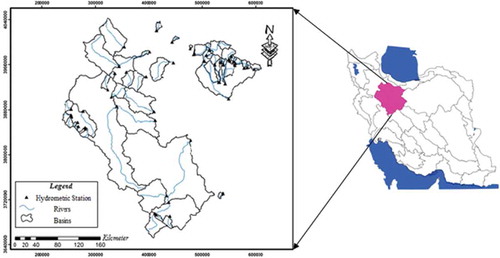
Figure 2. Structure of ANFIS used in this study.

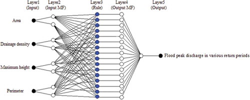
Input fuzzification is carried out in the first layer; the nodes are fixed nodes in the second (multiplies incoming signals) and third (calculates the normalized firing strength) layers; and the nodes in the fourth layer are called adaptive nodes. Parameters are referred to as consequent parameters. The fifth layer is a single fixed node, which computes the overall output by summing all incoming signals. In the present study, the triangular, trapezoidal, sigmoidal, generalized bell-shaped, Gaussian and Gaussian2 membership functions (MFs) were applied. In each application, different numbers of MFs were tried, and the best one, giving the minimum of errors, was selected. More information on ANFIS can be found in Jang (1993).

2.2.5 Standardization of data

In this study, before the training of the models, both input and output variables were normalized within the range 0.1–0.9 as follows:

(15)

where N_i is the normalized value of a certain parameter, x_i is the measured value for this parameter, and x_min and x_max are, respectively, the minimum and maximum values in the database for this parameter (Dogan et al. 2010, Besalatpour et al. 2013).

2.2.6 Evaluation of model performance

To assess the model performance, three statistical criteria, root mean squared error (RMSE), Nash-Sutcliffe coefficient of efficiency (NSC) and coefficient of determination (R²) were used as follows:

(16)

(17)

(18)

where q_o(t) is the observed discharge for a certain period, t; q_p(t) is the predicted discharge; n is the number of observed data; and and are, respectively, the observed and the predicted mean discharge for a certain period, t.

Legates and McCabe (1999) showed that the coefficient of determination (R²) alone is not appropriate to evaluate the goodness-of-fit of model simulations. Therefore, other statistical indexes, for example, RMSE and NSC, should be applied to evaluate the models’ performance. The RMSE describes the average magnitude of the errors by attributing more weight to large errors; it ranges between 0 and ∞, with lower values corresponding to better model performance. The NSC can also provide good insight into the performance of a model. The optimal value of the NSC is 1, representing the best fit of the applied model to the observed data. The combined use of these measures can provide good insight into model performance. As indicated by Legates and McCabe (1999), NSC and RMSE criteria can adequately be used to evaluate model simulations (Kisi et al. 2013, Shiri et al. 2013).

3 Results and discussion

Table 2 shows the results obtained from the selected pdfs. As can be seen from Table 2, log-Pearson Type III had the lowest summing scores and the highest first rank and, therefore, was selected as the most suitable regional distribution (Vasant and Talegaokar 2014).

Table 2. Summing scores and the number of first rank for the selected pdfs in the studied area.

Statistical distribution	Log Pearson Type III	Three-parameter log normal	Two-parameter log normal	Pearson Type III	Two-parameter gamma	Gumbel	Normal
Summing scores	139	161	236	232	215	258	308
Total of first rank	17	12	6	6	5	4	4

To determine more important variables, the gamma value was calculated based on omitting variables one by one. Omitting important variables results in increasing gamma value in comparison with the gamma value of other variables. The results for different combinations are shown in Table 3.

Table 3. Gamma test results.

Variable	Gamma value	Variable	Gamma value
All inputs–A	0.2077	All inputs–WS	0.1782
All inputs–DD	0.2020	All inputs–Hmean	0.1773
All inputs–Hmax	0.1950	All inputs–R24	0.1773
All inputs–P	0.1844	All inputs–SL	0.1767
All inputs–IPF	0.1840	All inputs–SS	0.1752
All inputs–IR	0.1832	All inputs–T	0.1706
All inputs–RA	0.1820	All inputs–W	0.1697
All inputs–GR	0.1807	All inputs–U	0.1645
All inputs–R	0.1792	All inputs–DR	0.1635
All inputs–E	0.1787	All inputs–Hmin	0.1599

See Table 1 for definition of variables.

As can be seen from Table 3, area, drainage density, maximum height and perimeter are the best input combination for RFFA, having the highest gamma value. Selection of variables using GT was considered as the first strategy (Strategy A). Since the selected variables using GT are physiographical characteristics, a second strategy (Strategy B) was used to compare with GT. In Strategy B, one variable with high gamma value was selected from each of the physiographic, meteorological, geological and land-use characteristics through considering the GT results (Table 3). Accordingly, area (from the physiographic characteristics), annual mean rainfall (meteorological characteristics), impermeable formation area (geological characteristics) and irrigated farming area (land-use characteristics) were selected as the best input combination. In addition, the selection of variables was considered based on expert opinion (Strategy C). Accordingly, area, impermeable formation area, maximum 24-h rainfall and rangeland area were chosen as the best input combination.

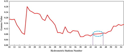
In addition, the suitable number of data points required for training and testing the model was determined using the M-test. The results obtained from M-test analysis are shown in Figure 3. In Figure 3, there is a clear stabilizing of the gamma statistic with a value of 0.08 between data points 43 and 47. Thus, we selected data point 45 as the marginal point for determination of training and testing data. Accordingly, samples (hydrometric stations) of training and testing sets were determined, respectively, as 45 and 10.

Figure 3. M-test diagram gamma value.

The optimal values of the parameters used in SVR are given in Table 4 for the three strategies. The constant-cost C and the radius of the insensitive tube ε are the nonlinear SVR parameter and the kernel parameter. These parameters are mutually dependent, so changing the value of one parameter changes other parameters. In this study, to determine parameters γ and d by trial-and-error method and for optimization of parameters C and ε, a grid search algorithm, namely a two-step grid search method with 10-fold cross-validation, was used. A two-step grid search algorithm, dividing the search process in two stages, was used to solved this problem. First, the search space becomes smaller, therefore determining the best region. Then the optimum parameters in the smaller search space are searched until finally optimal values of parameters are determined (Chen and Yu 2007). For 10-fold cross-validation, the hydrometric stations were divided into 10 subsets, and the leave-one-out (LOO) validation method was repeated 10 times. Each repetition, one of the 10 subsets was used as the test set and the other nine subsets were put together to form a training set. Then the average error across all 10 trials was computed. SVR models with these parameters were simulated, and the best-performing were selected.

Table 4. Optimal values of the parameters used in SVR.

Return period (years)	Strategy	Optimal values of parameters
		C	ε	γ	d
2	A	60	0.50	3.20	–
	B	60	0.60	1.45	2
	C	80	0.50	1.80	4
5	A	60	0.50	3.00	–
	B	5	0.32	1.10	3
	C	80	0.40	2.20	4
10	A	60	0.50	3.10	–
	B	45	0.70	1.30	2
	C	75	0.49	1.70	4
25	A	55	0.35	1.20	–
	B	40	0.30	0.85	–
	C	30	0.44	0.91	4
50	A	60	0.35	1.20	–
	B	30	0.32	1.15	2
	C	40	0.52	0.73	3
100	A	80	0.55	1.20	–
	B	125	0.38	1.48	–
	C	5	0.42	2.10	2

C: cost parameter; ε: radius of the insensitive tube; γ: gamma; d: degree.

Tables 5–8 show the performance of the SVR, ANFIS, ANN and NLR models, respectively, in the test phase, for the three strategies through the statistical indicators R², RMSE and NSC.

As can be seen from Table 5, the RBF kernel for the SVR model performed better than the other kernels in all return periods. This finding is in agreement with those of Moghadamnia et al. (2009a), Goel and Pal (2012) and Ibrahim and Wibowo (2014). As shown in Table 6, the generalized bell-shaped (Gbell) membership function for the ANFIS model, at return periods of 2, 5 and 10 years, is the best fuzzification function. This finding supports previous research (Wu and Kuo 2010), which used the Gbell membership function. For return periods of 25, 50 and 100 years, the Gaussian2 membership function was selected. This seems to be consistent with other research (Soyguder and Alli 2009, Zheng et al. 2011, Kisi et al. 2013).

Table 5. Results of SVR for the test phase.

Return period (years)	Strategy	Kernel function	R^2	RMSE (m^3/s)	NSC
2	A	RBF	0.91	11.32	0.82
	B	Polynomial	0.91	23.26	0.21
	C	Polynomial	0.93	11.55	0.80
5	A	RBF	0.90	17.57	0.84
	B	Polynomial	0.57	37.13	0.28
	C	Polynomial	0.85	19.33	0.81
10	A	RBF	0.92	23.97	0.82
	B	Polynomial	0.77	45.82	0.34
	C	Polynomial	0.88	26.68	0.78
25	A	RBF	0.89	37.37	0.76
	B	RBF	0.86	58.64	0.40
	C	Polynomial	0.79	42.40	0.68
50	A	RBF	0.82	45.84	0.76
	B	Polynomial	0.83	59.74	0.57
	C	Polynomial	0.69	74.31	0.34
100	A	RBF	0.76	58.84	0.71
	B	RBF	0.72	62.58	0.67
	C	Polynomial	0.49	89.74	0.32

RBF: radial basis function. Bold values indicate the best performance in terms of R², RMSE and NSC.

Table 6. Results of ANFIS for the test phase.

Return period (years)	Strategy	Membership function	MF	Epoch	R^2	RMSE (m^3/s)	NSC
2	A	Gbell	2	24	0.95	8.40	0.90
	B	Triangular	2	18	0.51	24.10	0.14
	C	Triangular	2	10	0.85	11.80	0.80
5	A	Gbell	2	25	0.90	18.24	0.82
	B	Trapezoidal	2	1	0.83	40.25	0.14
	C	Gaussian2	2	83	0.86	17.67	0.84
10	A	Gbell	2	23	0.85	26.95	0.77
	B	Triangular	2	11	0.23	53.66	0.01
	C	Triangular	2	3	0.70	31.32	0.69
25	A	Gaussian2	2	2	0.87	32.82	0.81
	B	Gaussian	2	26	0.73	53.10	0.51
	C	Triangular	2	21	0.80	35.36	0.78
50	A	Gaussian2	2	1	0.81	45.58	0.75
	B	Gaussian	2	27	0.80	46.20	0.74
	C	Triangular	2	16	0.71	52.66	0.67
100	A	Gaussian2	2	5	0.82	49.00	0.80
	B	Gaussian	2	39	0.81	55.27	0.74
	C	Gbell	2	17	0.73	68.19	0.61

Bold values indicate the best performance in terms of R², RMSE and NSC. Gbell: generalized bell-shaped.

The summary of results obtained from the best models (Tables 5–8) is shown in Table 9. Table 9 shows that SVR and ANFIS have similar performance and can be used to successfully estimate flood discharge. A possible explanation for this might be that ANFIS combines the capabilities of fuzzy logic and ANN in modelling, especially in RFFA. However, SVR uses the kernel function to model nonlinear relationships. Since flood magnitudes with different return periods are nonlinear, and exhibit a high degree of spatial and temporal variability, SVR and ANFIS models could guarantee achievement of nonlinearity in modelling. The present finding seems to be consistent with other research in this field (Shu and Ouarda 2008, Wu et al. 2008, Dogan et al. 2010, He et al. 2014).

Table 7. Results of ANN for the test phase.

Return period (years)	Strategy	Structure	Hidden layer	Output layer	Epoch	R^2	RMSE (m^3/s)	NSC
2	A	4-9-1	Tanh	Pureline	28	0.96	16.37	0.60
	B	4-3-1	Logistic	Pureline	11	0.67	22.62	0.25
	C	4-3-1	Logistic	Pureline	19	0.87	24.13	0.14
5	A	4-11-1	Logistic	Pureline	21	0.94	28.52	0.57
	B	4-10-1	Logistic	Pureline	17	0.82	27.43	0.60
	C	4-11-1	Tanh	Pureline	20	0.92	31.16	0.48
10	A	4-9-1	Tanh	Pureline	46	0.97	27.10	0.70
	B	4-9-1	Tanh	Pureline	15	0.90	36.22	0.59
	C	4-8-1	Tanh	Pureline	16	0.85	40.93	0.48
25	A	4-8-1	Logistic	Pureline	24	0.85	49.13	0.58
	B	4-2-1	Tanh	Pureline	92	0.89	49.30	0.57
	C	4-2-1	Tanh	Pureline	15	0.81	56.74	0.44
50	A	4-12-1	Tanh	Pureline	40	0.85	54.28	0.65
	B	4-4-1	Logistic	Pureline	26	0.84	56.00	0.62
	C	4-11-1	Tanh	Pureline	12	0.76	67.50	0.45
100	A	4-4-1	Logistic	Pureline	34	0.80	75.90	0.51
	B	4-12-1	Tanh	Pureline	15	0.79	69.80	0.59
	C	4-6-1	Tanh	Pureline	13	0.78	68.52	0.60

Bold values indicate the best performance in terms of R², RMSE and NSC.

Table 8. Results of NLR for the test phase.

Return period (years)	Strategy	R^2	RMSE (m^3/s)	NSC
2	A	0.91	22.00	0.28
	B	0.95	13.42	0.74
	C	0.86	25.77	0.02
5	A	0.93	32.46	0.44
	B	0.97	20.92	0.77
	C	0.94	36.00	0.31
10	A	0.91	39.98	0.50
	B	0.93	37.21	0.57
	C	0.94	41.11	0.47
25	A	0.88	50.66	0.55
	B	0.85	53.02	0.51
	C	0.89	46.87	0.61
50	A	0.85	63.54	0.51
	B	0.79	68.92	0.43
	C	0.85	50.45	0.69
100	A	0.75	58.24	0.71
	B	0.74	80.80	0.45
	C	0.80	53.26	0.76

Bold values indicate the best performance in terms of R², RMSE and NSC.

Table 9. Comparison of statistics of each model in the test period.

Return period (years)	Model
	SVR			St.	ANFIS			St.	ANN			St.	NLR			St.
	R^2	RMSE	NSC		R^2	RMSE	NSC		R^2	RMSE	NSC		R^2	RMSE	NSC
2	0.91	11.32	0.82	A	0.95	8.40	0.90	A	0.94	16.64	0.60	A	0.95	13.42	0.74	B
5	0.90	17.57	0.84	A	0.90	18.24	0.82	A	0.82	27.43	0.60	B	0.97	20.92	0.77	B
10	0.92	23.97	0.82	A	0.85	26.95	0.77	A	0.97	27.10	0.70	A	0.93	37.21	0.57	B
25	0.89	37.37	0.76	A	0.87	32.82	0.81	A	0.85	49.13	0.58	A	0.89	46.87	0.61	C
50	0.82	45.84	0.76	A	0.81	45.58	0.75	A	0.85	54.28	0.65	A	0.85	50.45	0.69	C
100	0.76	58.84	0.71	A	0.82	49.00	0.80	A	0.78	68.52	0.60	C	0.80	53.26	0.76	C

Bold values indicate the best performance in terms of R², RMSE and NSC. St.: strategy.

Table 10. Performance of the developed models.

Return period (years)	Model
	SVR	ANFIS	ANN	NLR
2	Very good	Very good	Satisfactory	Good
5	Very good	Very good	Satisfactory	Very good
10	Very good	Very good	Good	Satisfactory
25	Very good	Very good	Satisfactory	Good
50	Very good	Very good	Satisfactory	Good
100	Good	Very good	Satisfactory	Very good

In general, selection of variables using GT (Strategy A) produced better results than the other two strategies. Moriasi et al. (2007) suggested a quality class for watershed models using NSC (Fatehi et al. 2015). Therefore, the developed models were classified using this approach i.e. NSC ≤ 0.50 (Unsatisfactory), 0.50 < NSC ≤ 0.65 (Satisfactory), 0.65 < NSC ≤ 0.75 (Good) and 0.75 < NSC ≤ 1.00 (Very good) (Table 10).

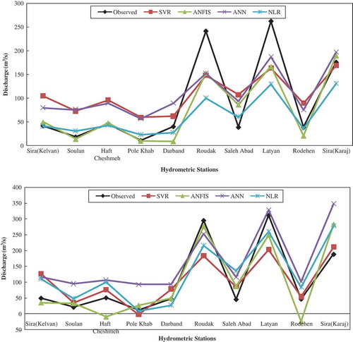
As shown in Table 10, the selected models (Table 9) were classified between Satisfactory and Very good. The SVR and ANFIS models are classified as Good and Very good, but the majority of ANN and NLR models are classified as Satisfactory and Good. Figure 4 shows the observed and estimated data for different return periods in the test phase.

Figure 4. Graph of observed and estimated data for different return periods (Tr) in the test phase.

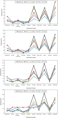
Figure 4. (Continued).

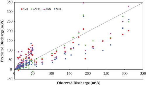
A qualitative assessment of various RFFA models is shown in Figure 5. As can be seen from Figure 5, the difference in prediction appears to increase with increase in return period. However, there is a minor difference in prediction between NLR and ANFIS models, while a large difference in prediction is observed particularly between ANN model and other models. The scatter plots of observed and estimated flood discharge using various RFFA models are shown in Figure 6. As shown in Figure 6, there is a slight difference for predicting flood discharge lower than 100 m³ s⁻¹.

Figure 5. A comparison of RFFA models (a) on ordinary scale, and (b) on semi-log scale in the test phase.

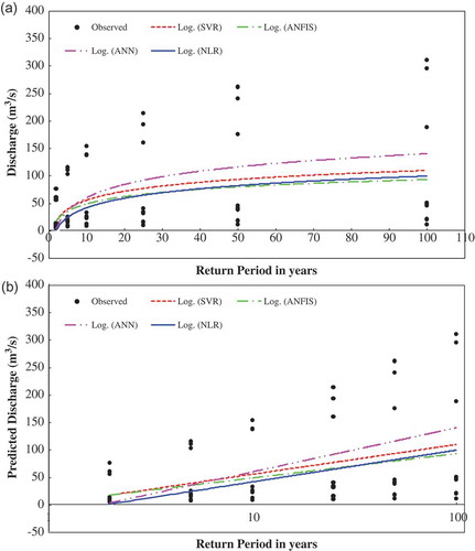
Figure 6. Estimated vs observed flood discharge for different return periods in the test phase.

4 Conclusions

In this paper, we compared the SVR, ANFIS, ANN and NLR models for RFFA in the Namak Lake watershed, Iran. The study was carried out using data of 55 hydrometric stations for the 20-year period between 1992/93 and 2011/12. The Kolmogorov-Smirnov test was used to rank probability distribution functions (pdfs) for estimating flood discharge with a certain return period. Hence, the log-Pearson Type III distribution was selected as the best pdf with the minimum error. Three strategies, GT, GT + classification and expert opinion, were used to select variables. Finally, the GT technique was selected as the best strategy. Indeed the GT reduces numbers of variables and provides the essential input variables for modelling. Therefore, area, drainage density, maximum height and perimeter were selected using GT as input variables. This study has found that, generally, the RBF kernel for SVR models performed better than the other kernels. The second major finding was that the Gbell membership function for ANFIS in return periods of 2, 5 and 10 years is the best fuzzification function. For return periods of 25, 50 and 100 years, the Gaussian2 membership function performed better than the other functions. These findings suggest that SVR and ANFIS have similar performance and can be used to successfully estimate flood discharge in the study region. Since the estimated return period quantiles refer to return periods of up to 100 years based on a 20-year record, further research is required to be conducted with longer time series.

Disclosure statement

No potential conflict of interest was reported by the authors.

References

- Afiq, H., et al., 2013. Daily forecasting of dam water levels: comparing a support vector machine (SVM) model with adaptive neuro fuzzy inference system (ANFIS). Water Resources Management, 27, 3803–3823. doi:10.1007/s11269-013-0382-4
- Ahn, J., et al., 2014. Flood frequency analysis for the annual peak flows simulated by an event-based rainfall-runoff model in an urban drainage basin. Water, 6 (12), 3841–3863. doi:10.3390/w6123841
- Alobaidi, M.H., et al., 2015. Regional frequency analysis at ungauged sites using a two-stage resampling generalized ensemble framework. Advances in Water Resources, 84, 103–111. doi:10.1016/j.advwatres.2015.07.019
- Asefa, T., et al., 2006. Multi-time scale stream flow predictions: the support vector machines approach. Journal of Hydrology, 318 (1–4), 7–16. doi:10.1016/j.jhydrol.2005.06.001
- Aziz, K., et al., 2014. Application of artificial neural networks in regional flood frequency analysis: a case study for Australia. Stochastic Environmental Research and Risk Assessment, 28 (3), 541–554. doi:10.1007/s00477-013-0771-5
- Aziz, K., et al., 2017. Flood estimation in ungauged catchments: application of artificial intelligence based methods for Eastern Australia. Stochastic Environmental Research and Risk Assessment, 31 (6), 1499–1514. doi:10.1007/s00477-016-1272-0
- Aziz, K., Rai, S., and Rahman, A., 2015. Design flood estimation in ungauged catchments using genetic algorithm-based artificial neural network (GAANN) technique for Australia. Natural Hazards, 77 (2), 805–821. doi:10.1007/s11069-015-1625-x
- Besalatpour, A., et al., 2013. Estimating wet soil aggregate stability from easily available properties in a highly mountainous watershed. Catena, 111, 72–79. doi:10.1016/j.catena.2013.07.001
- Blöschl, G. and Sivapalan, M., 1997. Process controls on regional flood frequency: coefficient of variation and basin scale. Water Resources Research, 33 (12), 2967–2980. doi:10.1029/97WR00568
- Bozchaloei, S.K. and Vafakhah, M., 2015. Regional analysis of flow duration curves using adaptive neuro-fuzzy inference system. Journal of Hydrologic Engineering, 20 (12), 06015008. doi:10.1061/(ASCE)HE.1943-5584.0001243
- Bray, M. and Han, D., 2004. Identification of support vector machines for runoff modelling. Journal of Hydroinformatics, 6 (4), 265–280.
- Chau, K., Wu, C., and Li, Y., 2005. Comparison of several flood forecasting models in Yangtze River. Journal of Hydrologic Engineering, 10 (6), 485–491. doi:10.1061/(ASCE)1084-0699(2005)10:6(485)
- Chen, S.-H., et al., 2006. The strategy of building a flood forecast model by neuro-fuzzy network. Hydrological Processes, 20 (7), 1525–1540. doi:10.1002/(ISSN)1099-1085
- Chen, S.-T. and Yu, P.-S., 2007. Real-time probabilistic forecasting of flood stages. Journal of Hydrology, 340 (1–2), 63–77. doi:10.1016/j.jhydrol.2007.04.008
- Cobaner, M., Unal, B., and Kisi, O., 2009. Suspended sediment concentration estimation by an adaptive neuro-fuzzy and neural network approaches using hydro-meteorological data. Journal of Hydrology, 367 (1–2), 52–61. doi:10.1016/j.jhydrol.2008.12.024
- Dalrymple, T., 1960. Flood-frequency analyses, manual of hydrology: part 3. Washington, DC: USGPO.
- Dawson, C.W., et al., 2006. Flood estimation at ungauged sites using artificial neural networks. Journal of Hydrology, 319 (1–4), 391–409. doi:10.1016/j.jhydrol.2005.07.032
- Dibike, Y.B., et al., 2001. Model induction with support vector machines: introduction and applications. Journal of Computing in Civil Engineering, 15 (3), 208–216. doi:10.1061/(ASCE)0887-3801(2001)15:3(208)
- Dogan, E., et al., 2010. Modelling of evaporation from the reservoir of Yuvacik dam using adaptive neuro-fuzzy inference systems. Engineering Applications of Artificial Intelligence, 23 (6), 961–967. doi:10.1016/j.engappai.2010.03.007
- Durrant, P.J., 2001. winGamma TM: a non-linear data analysis and modelling tool with applications to flood prediction. Citeseer. PhD dissertation, Department of Computer Science, Cardiff University, Wales, UK.
- Fatehi, I., et al., 2015. Modeling the relationship between catchment attributes and in-stream water quality. Water Resources Management, 29 (14), 5055–5072. doi:10.1007/s11269-015-1103-y
- Ghafari, G. and Vafakhah, M., 2012. Rainfall-runoff modeling using artificial neural networks and adaptive neuro-fuzzy inference system models. In: C. Kahraman, E.E. Kerre, and F.T. Bozbura, eds. Uncertainty modeling in knowledge engineering and decision making. Singapore: World Scientific, 951–956.
- Gizaw, M.S. and Gan, T.Y., 2016. Regional flood frequency analysis using support vector regression under historical and future climate. Journal of Hydrology, 538, 387–398. doi:10.1016/j.jhydrol.2016.04.041
- Goel, A. and Pal, M., 2012. Stage-discharge modeling using support vector machines. International Journal of Engineering, 25 (1), 1–9. doi:10.5829/idosi.ije.2012.25.01a.01
- He, Z., et al., 2014. A comparative study of artificial neural network, adaptive neuro fuzzy inference system and support vector machine for forecasting river flow in the semiarid mountain region. Journal of Hydrology, 509, 379–386. doi:10.1016/j.jhydrol.2013.11.054
- Hosking, J.R.M. and Wallis, J.R., 2005. Regional frequency analysis: an approach based on L-moments. New York: Cambridge University Press.
- Ibrahim, N. and Wibowo, A., 2014. Support vector regression with missing data treatment based variables selection for water level prediction of Galas River in Kelantan Malaysia. Wseas Transactions on Mathematics, 13 (1), 69–78.
- Jang, J.-S.R., 1993. ANFIS: adaptive-network-based fuzzy inference system. IEEE Transactions on Systems, Man and Cybernetics, 23 (3), 665–685. doi:10.1109/21.256541
- Jang, J.-S.R., Sun, C.-T., and Mizutani, E., 1997. Neuro-fuzzy and soft computing; a computational approach to learning and machine intelligence. 1 ed. Upper Saddle River, NJ: Prentice Hall.
- Jingyi, Z. and Hall, M., 2004. Regional flood frequency analysis for the Gan-Ming River basin in China. Journal of Hydrology, 296 (1–4), 98–117. doi:10.1016/j.jhydrol.2004.03.018
- Kalteh, A.M., 2013. Monthly river flow forecasting using artificial neural network and support vector regression models coupled with wavelet transform. Computers & Geosciences, 54, 1–8. doi:10.1016/j.cageo.2012.11.015
- Kheirfam, H. and Vafakhah, M., 2015. Assessment of some homogeneous methods for the regional analysis of suspended sediment yield in the south and southeast of the Caspian Sea. Journal of Earth System Science, 124 (6), 1247–1263. doi:10.1007/s12040-015-0604-7
- Kişi, Ö., 2006. Daily pan evaporation modelling using a neuro-fuzzy computing technique. Journal of Hydrology, 329 (3–4), 636–646. doi:10.1016/j.jhydrol.2006.03.015
- Kisi, O., Shiri, J., and Tombul, M., 2013. Modeling rainfall-runoff process using soft computing techniques. Computers & Geosciences, 51, 108–117. doi:10.1016/j.cageo.2012.07.001
- Kisi, O., Yuksel, I., and Dogan, E., 2008. Modelling daily suspended sediment of rivers in Turkey using several data-driven techniques. Hydrological Sciences Journal, 53 (6), 1270–1285. doi:10.1623/hysj.53.6.1270
- Kurtulus, B. and Razack, M., 2010. Modeling daily discharge responses of a large karstic aquifer using soft computing methods: artificial neural network and neuro-fuzzy. Journal of Hydrology, 381 (1–2), 101–111. doi:10.1016/j.jhydrol.2009.11.029
- Legates, D.R. and McCabe, G.J., 1999. Evaluating the use of “goodness-of-fit” measures in hydrologic and hydroclimatic model validation. Water Resources Research, 35 (1), 233–241. doi:10.1029/1998WR900018
- Lin, J.-Y., Cheng, C.-T., and Chau, K.-W., 2006. Using support vector machines for long-term discharge prediction. Hydrological Sciences Journal, 51 (4), 599–612. doi:10.1623/hysj.51.4.599
- Liong, S.-Y. and Sivapragasam, C., 2002. Flood stage forecasting with support vector machines. Journal of the American Water Resources Association, 38 (1), 173–186. doi:10.1111/jawr.2002.38.issue-1
- Moghaddamnia, A., et al., 2009a. Evaporation estimation using support vector machines technique. International Journal of Engineering and Applied Sciences, 5 (7), 415–423.
- Moghaddamnia, A., et al., 2009b. Evaporation estimation using artificial neural networks and adaptive neuro-fuzzy inference system techniques. Advances in Water Resources, 32 (1), 88–97. doi:10.1016/j.advwatres.2008.10.005
- Moriasi, D.N., Arnold, J.G., Van Liew, M.W., Bingner, R.L., Harmel, R.D., and Veith, T.L., 2007. Model evaluation guidelines for systematic quantification of accuracy in watershed simulations. Transactions of the ASABE, 50 (3), 885–900. doi:10.13031/2013.23153
- Nayak, P.C., et al., 2004. A neuro-fuzzy computing technique for modeling hydrological time series. Journal of Hydrology, 291 (1–2), 52–66. doi:10.1016/j.jhydrol.2003.12.010
- Noori, R., et al., 2011. Assessment of input variables determination on the SVM model performance using PCA, Gamma test, and forward selection techniques for monthly stream flow prediction. Journal of Hydrology, 401 (3–4), 177–189. doi:10.1016/j.jhydrol.2011.02.021
- Pallard, B., Castellarin, A., and Montanari, A., 2009. A look at the links between drainage density and flood statistics. Hydrology and Earth System Sciences, 13 (7), 1019–1029. doi:10.5194/hess-13-1019-2009
- Rahman, A., Haddad, K., and Eslamian, S., 2014. Regional flood frequency analysis. In: S. Eslamian, ed. Handbook of engineering hydrology: modeling, climate change, and variability. Boca Raton, FL: CRC Press, 451–469.
- Seckin, N. and Guven, A., 2012. Estimation of peak flood discharges at ungauged sites across Turkey. Water Resources Management, 26, 2569–2581. doi:10.1007/s11269-012-0033-1
- Shiri, J., et al., 2013. Predicting groundwater level fluctuations with meteorological effect implications—a comparative study among soft computing techniques. Computers & Geosciences, 56, 32–44. doi:10.1016/j.cageo.2013.01.007
- Shu, C. and Burn, D.H., 2004. Artificial neural network ensembles and their application in pooled flood frequency analysis. Water Resources Research, 40 (9). doi:10.1029/2003WR002816
- Shu, C. and Ouarda, T.B.M.J., 2007. Flood frequency analysis at ungauged sites using artificial neural networks in canonical correlation analysis physiographic space. Water Resources Research, 43, W07438. doi:10.1029/2006WR005142
- Shu, C., and Ouarda, T.B.M.J., 2008. Regional flood frequency analysis at ungauged sites using the adaptive neuro-fuzzy inference system. Journal of Hydrology, 349 (1–2), 31–43. doi:10.1016/j.jhydrol.2007.10.050
- Soyguder, S. and Alli, H., 2009. Predicting of fan speed for energy saving in HVAC system based on adaptive network based fuzzy inference system. Expert Systems with Applications, 36 (4), 8631–8638. doi:10.1016/j.eswa.2008.10.033
- Srinivas, V., et al., 2008. Regional flood frequency analysis by combining self-organizing feature map and fuzzy clustering. Journal of Hydrology, 348 (1–2), 148–166. doi:10.1016/j.jhydrol.2007.09.046
- Stedinger, J.R. and Griffis, V.W., 2008. Flood frequency analysis in the United States: time to update. Journal of Hydrologic Engineering, 13 (4), 199–204. doi:10.1061/(ASCE)1084-0699(2008)13:4(199)
- Talei, A., Chua, L.H.C., and Wong, T.S., 2010. Evaluation of rainfall and discharge inputs used by Adaptive Network-based Fuzzy Inference Systems (ANFIS) in rainfall–runoff modeling. Journal of Hydrology, 391 (3–4), 248–262. doi:10.1016/j.jhydrol.2010.07.023
- Vafakhah, M., 2012. Application of artificial neural networks and adaptive neuro-fuzzy inference system models to short-term streamflow forecasting. Canadian Journal of Civil Engineering, 39 (4), 402–414. doi:10.1139/l2012-011
- Vafakhah, M. and Eslamian, S., 2014. Regionalization of hydrological variables. In: S. Eslamian, ed. Handbook of engineering hydrology: modeling, climate change, and variability. Boca Raton, FL: CRC Press, 471–499.
- Vafakhah, M. and Kahneh, E., 2016. A comparative assessment of adaptive neuro-fuzzy inference system, artificial neural network and regression for modelling stage-discharge relationship. International Journal of Hydrology Science and Technology, 6 (2), 143–159. doi:10.1504/IJHST.2016.075581
- Vasant, S.A. and Talegaokar, S., 2014. Hydrological study of man (Chandrabhaga) river. International Journal of Advances in Engineering & Technology, 7 (3), 807–817.
- Wu, C., Chau, K., and Li, Y., 2008. River stage prediction based on a distributed support vector regression. Journal of Hydrology, 358 (1–2), 96–111. doi:10.1016/j.jhydrol.2008.05.028
- Wu, J.-D. and Kuo, J.-M., 2010. Fault conditions classification of automotive generator using an adaptive neuro-fuzzy inference system. Expert Systems with Applications, 37 (12), 7901–7907. doi:10.1016/j.eswa.2010.04.046
- Yilmaz, I. and Kaynar, O., 2011. Multiple regression, ANN (RBF, MLP) and ANFIS models for prediction of swell potential of clayey soils. Expert Systems with Applications, 38 (5), 5958–5966. doi:10.1016/j.eswa.2010.11.027
- Yu, P.-S., Chen, S.-T., and Chang, I.-F., 2006. Support vector regression for real-time flood stage forecasting. Journal of Hydrology, 328 (3–4), 704–716. doi:10.1016/j.jhydrol.2006.01.021
- Zheng, H., Jiang, B., and Lu, H., 2011. An adaptive neural-fuzzy inference system (ANFIS) for detection of bruises on Chinese bayberry (Myrica rubra) based on fractal dimension and RGB intensity color. Journal of Food Engineering, 104 (4), 663–667. doi:10.1016/j.jfoodeng.2011.01.031