Estimating uncertainty of streamflow measurements with moving-boat acoustic Doppler current profilers

ABSTRACT

A theoretical and a semi-empirical model are presented for estimating the uncertainty of streamflow measurements made with an acoustic Doppler current profiler (ADCP) mounted on a moving platform. Both models are based on the statistical analysis of ADCP ensemble discharge time series collected during a transect; therefore, they account for all random error sources associated with the measurement at a site. The theoretical model is developed based on the law of propagation of variance; it explores the theoretical relationship between the variables involved in the problem. The semi-empirical model is developed based on the theory of dimensional analysis; it explores the empirical relationship between the variables. The semi-empirical model is calibrated using 205 transect datasets and verified with an additional 382 transect datasets. It provides a useful tool for the uncertainty analysis and uncertainty-based measurement quality control of moving-boat ADCP streamflow measurements.

KEYWORDS:

• ADCP
• discharge measurement
• random errors
• streams and rivers
• uncertainty

Editor A. Castellarin; Associate editor I. Overton

1 Introduction

The estimation of the uncertainty of streamflow measurements made with an acoustic Doppler current profiler (ADCP) mounted on a moving platform is an important task. This is because uncertainty is an import indicator of measurement quality (JCGM 2008). For a measured discharge (like any measurement result) to be meaningful, it must be accompanied by a statement of its uncertainty. Moreover, according to the ADCP measurement quality assurance policies implemented by water resources agencies (e.g. USGS 2002, EC 2004, MWR 2006, Mueller et al. 2013), a measured discharge must meet an acceptance criterion. An uncertainty-based acceptance criterion was recently proposed for statistical quality control of moving-boat ADCP streamflow measurements (Huang 2015).

According to the traditional classification of random and systematic uncertainty sources, measurement uncertainty can be divided into two components: one due to random error sources and the other due to bias error sources. The major sources of random errors associated with ADCP streamflow measurements include ADCP system noise in depth and velocity measurements, pitch, roll and heading variation/errors, and ambient turbulence; the bias error can be separated into three classes: instrument error, operator error, and moving-bed error (Huang 2015). Detailed discussions on the error sources can be found in Simpson (2001), González-Castro and Muste (2007), and Huang (2012). González-Castro and Muste (2007) presented an uncertainty analysis framework based on the law of propagation of uncertainty to estimate the bias limit (i.e. the uncertainty component due to bias error sources) and statistical analysis of multiple transect discharge data to estimate the precision limit (i.e. the uncertainty component due to random error sources). The validation study of Oberg and Mueller (2007), which essentially considered the instrument and operator errors, showed that streamflow measurements with broadband ADCPs were unbiased when compared to the reference discharges. The validation study of Boldt and Oberg (2015) showed that streamflow measurements with two new ADCP models (M9 and RiverRay) were not biased relative to the reference measurements. The moving-bed error, which causes the negative bias in discharge measurements, can be addressed by using a GPS (e.g. Rennie and Rainville 2006, Wagner and Mueller 2011), the loop method (Mueller and Wagner 2007) or the stationary ADCP method (Huang 2012). The bias error due to the operator or moving bed must be addressed or eliminated by following guidance on field procedures (e.g. Mueller et al. 2013). The uncertainty due to bias error sources is not a subject of this paper. This paper considers the uncertainty due to random error sources only.

It should be mentioned that ISO 5168 (2005) started to use the Type A and Type B terminology for uncertainty classification to comply with the Guide to the Expression of Uncertainty in Measurement (GUM) (JCGM 2008). Type A evaluations of uncertainty are those using statistical methods, specifically those that use the spread of a number of measurements, while Type B evaluations of uncertainty are those carried out by means other than the statistical analysis of series of observations (ISO 5168 2005). However, ISO 5168 (2005) still observes the traditional classification of random and systematic uncertainty sources. Each classification has its own advantages in terms of describing the physics and mathematics involved in uncertainty analysis; the use of both terminologies may help in understanding the nature or characteristics of error sources from different points of view (Huang 2013). The difference in terminology may not make a substantial difference in the final results of uncertainty analysis. Both terminologies are used in this paper.

A moving-boat ADCP streamflow measurement under steady flow conditions usually involves multiple transects to obtain a set of transect discharges. In this situation, the random uncertainty of the measured discharge can be estimated by statistical analysis of the transect discharge data. This is the Type A evaluation of uncertainty according to ISO 5168 (2005) and GUM (JCGM 2008) (Huang 2016).

Two recent studies focused on ADCP data quality evaluation or measurement uncertainty assessment. Mueller (2016a, 2016b) developed a computer program named QRev, which automates filtering and quality checking of the collected data. QRev estimates the random uncertainty based on transect discharge data (Type A evaluation) and the systematic uncertainty based on a user’s professional judgment (Type B evaluation). González-Castro et al. (2016) introduced RiverFlowUA, a GUI with capabilities to compute the mean discharge and total uncertainty. RiverFlowUA computes the total uncertainty by combining the random uncertainty estimated from transect discharge data (Type A evaluation) and the calibration uncertainties of the variables measured or derived by the ADCP measuring system based on the manufacturer’s specifications (Type B evaluation).

However, for measurements under unsteady flow conditions, such as on a tide-influenced river or during a flooding period, the Type A evaluation of uncertainty is impractical. In this situation, the uncertainty of a single transect discharge measurement may have to be estimated using an uncertainty model. Two models for estimating the uncertainty of a single transect discharge measurement are available in the literature. One is a simplified random-error model developed based on the law of propagation of uncertainty (Simpson 2001). The other is a modified Simpson model (Huang 2006, 2008). Both models do not use data collected by an ADCP at a site; therefore, they are Type B models. The two Type B models quantify major sources of random errors such as ADCP noise (in terms of the single ping standard deviation in velocity measurement), ambient turbulence, and cross-correlation between ADCP depth cells in velocity measurement. However, ambient turbulence and cross-correlation are not satisfactorily quantified in either of the models. In addition, because the data collected by an ADCP at a site are not used, the two Type B models do not reflect the site-specific measurement conditions.

García et al. (2012) presented a conceptual model for quantifying the random errors of moving-boat ADCP streamflow measurements associated with different sampling times. Tarrab et al. (2012) presented a systematic analysis quantifying the role of turbulence fluctuations using transect discharges generated from direct numerical simulation (DNS). However, neither the conceptual model nor the DNS has been implemented for estimating the uncertainty of a single transect discharge measurement.

Moore et al. (2017) presented a method for assessing uncertainty of ADCP discharge measurements using Monte Carlo simulations, considering both random and systematic errors (biases). The difficulty of using Monte Carlo simulation is that the simulation requires knowledge of the distribution of each input quantity associated with an error source. Their simulations helped to examine the contribution of each error source to the total uncertainty. However, they tested their method for datasets from 10 measurements only, and their results did not separate the uncertainty component due to random error sources from that due to bias error sources.

Huang (2012) presented a hybrid model for estimating the uncertainty of a single discharge measurement using the stationary ADCP method. The hybrid model consists of Type A and Type B uncertainty components. The Type A uncertainty component is estimated by statistical analysis of ADCP ensemble discharge time series collected at each vertical; therefore, the model accounts for site-specific measurement conditions. The Type B uncertainty component is estimated essentially in the same way as that in the Type B uncertainty model for the current-meter method (ISO 5168 2005, ISO 748 2007).

Cohn et al. (2013) presented an interpolated variance estimator (IVE) method for estimating the uncertainty of streamflow measurements with traditional current meters. The IVE method estimates the uncertainty based on the statistical analysis of velocity and depth data collected during streamflow measurement at a site. The advantage of the IVE method is that it captures all sources of random uncertainty in velocity and depth measurement; therefore, there is no need to quantify individual error sources (Cohn et al. 2013).

The idea of using ensemble discharge time series for uncertainty estimation of the stationary ADCP method (Huang 2012) is adopted and extended in this study to develop models for uncertainty estimation in the moving-boat ADCP method. The concept of the IVE for uncertainty estimation of the current-meter method (Cohn et al. 2013) is also adopted and extended. In this paper, we first present a theoretical model based on the law of propagation of variance. We then present a semi-empirical model based on the theory of dimensional analysis. The paper thereafter focuses on the semi-empirical model. We address the calibration and verification of the semi-empirical model, followed by discussion.

This paper assumes that readers are familiar with ADCP fundamentals and moving-boat ADCP streamflow measurements. Therefore, no discussions on ADCP technology, configuration, and measurement procedures are made. In addition, although all data used in this study were collected with Teledyne RD Instruments ADCPs, this paper deals with ADCPs in general, regardless of manufacturer or model.

2 Model development

The channel total discharge (denoted by Q) measured using the moving-boat ADCP method can be written as:

(1)

where Q_m is the channel main section discharge measured by an ADCP between the start point and the end point of a transect, and Q_re and Q_le are the right- and left-edge discharges, respectively.

Based on the law of propagation of variance, the relative standard uncertainty (RSU) of a single transect discharge measurement can be written as:

(2)

where var(Q_m) is the variance of the channel main section discharge, and var(Q_re) and var(Q_le) are the variances of the right- and left-edge discharges, respectively. The use of RSU is consistent with the uncertainty model for the current-meter method (ISO 5168 2005, ISO 748 2007, Cohn et al. 2013), and that for the stationary ADCP method (Huang 2012).

Equation (2) assumes that Q_m is uncorrelated with Q_re or Q_le. An ADCP uses edge ensemble velocity and depth data to calculate edge discharges (default setting of 10 edge ensembles in WinRiver II, the operation software of Teledyne RD Instruments ADCPs). The edge ensemble data are also included in the calculation of Q_m. However, the contribution of the edge ensembles to Q_m is usually near zero or negligible because edge ensembles should be collected when a boat or float is stationary. Therefore, it is reasonable to assume Q_m is uncorrelated with Q_re or Q_le.

The relative standard uncertainty of Q_m, denoted by RSU_m, is defined as:

(3)

Hereafter, we focus on developing the models for RSU_m. The formulation of the variances var(Q_re) and var(Q_le) and corresponding relative standard uncertainties of edge discharges are presented in Appendix 1.

2.1 A theoretical model for RSU_m

Mathematically, the discharge Q_m is an integral of the water velocity along the boat track of an ADCP transect (e.g. Christensen and Herrick 1982):

(4)

where S is the cross-sectional area along the boat track, u is the water velocity vector, and η is the unit vector normal to the boat’s track at a differential area ds.

An ADCP collects ensemble time series data for water velocity, boat velocity, and water depth when transecting a river. Ensemble discharges are calculated by the ADCP operation software in real time or in post-processing using the data. The integral in Equation (4) can be replaced by the summation of all ensemble discharges collected during a transect:

(5)

where q_i is the ensemble discharge at time (or location) i, and N is the number of total ensembles in the transect.

An ensemble discharge is a sum of three partial discharges: the top, middle, and bottom layer discharges. The middle layer discharge is calculated using the measured velocities at all valid cells in the ensembles; the top and bottom layer discharges are estimated using the velocity extrapolation (e.g. TRDI 2009). The selection of extrapolation methods may cause an uncertainty (mainly a bias) in estimated discharges (Huang 2012). A methodology and computer software named “extrap” for analysing the sensitivity of the discharge to extrapolation methods were developed by Mueller (2013). The uncertainty due to the selection of extrapolation methods is not considered in this study.

Equation (5) can be rewritten as:

(6)

where is the mean of the ensemble discharges collected during a transect:

(7)

The ensemble discharge q_i is a random variable. Its randomness is attributed to all random error sources associated with the measurement at a site. The collection of the ensemble discharge time series from multiple transects is a stochastic process. Thus, an ensemble discharge time series of a transect is a realization of the stochastic process. If we assume that an ensemble discharge time series is stationary, i.e. having a constant mean and variance for all i, the variance of Q_m can be estimated as:

(8)

If we further assume that the ensemble discharges are independent, the variance of can be calculated as the mean of the sample variance s²:

(9)

Thus, for an ensemble discharge time series that is stationary and uncorrelated, the variance var(Q_m) is simply:

(10)

However, an ensemble discharge time series is most likely neither stationary nor uncorrelated. It usually has a trend (i.e. a time-varying mean), a time-varying variance, and autocorrelation between ensembles (also known as serial correlation). A trend is often evident because the ensemble discharge usually increases when an ADCP is transecting from a bank to the middle of a river and decreases when transecting from the middle of the river to the other bank. A time-varying variance is also often evident because the random error in ensemble discharges is proportional to the magnitude of ensemble discharges; the variance is usually small near an edge where ensemble discharges are small and great in the middle of the river where ensemble discharges are large. The autocorrelation in an ensemble discharge time series without de-trending may be attributed to two factors: the trend and the eddy structure. It depends on the level of trends and the size of eddies with respect to the level of randomness (i.e. noises) of ensemble discharges.

First, we consider the autocorrelation and assume that an ensemble discharge time series is stationary. The variance of the sample mean of auto-correlated data will be biased (Law and Kelton 1991). We employ an unbiased estimator (Law and Kelton 1991) to estimate the variance of :

(11)

where γ_N is a constant (e.g. Law and Kelton 1991):

(12)

where ρ_i is the autocorrelation function (ACF) of ensemble discharge time series, i.e. the lag-i autocorrelation.

Next, we consider the nonstationarity. In statistics, the true variance of data is defined as the mean of squared errors. If the true ensemble discharge at i, denoted by , is known, s² can be calculated as:

(13)

It is impossible to know the true ensemble discharge; an estimator of has to be used. However, using an estimator will introduce a bias in the estimated variance s². Let denote the estimator of and ξ denote the estimator bias correction factor; Equation (13) is then rewritten as:

(14)

where ∆q_i is the ensemble discharge residual; .

The sum of the squared residuals in Equation (14) is known as the residual sum of squares (RSS) in statistics. The RSS is a measure of the discrepancy between the data and an estimation model (e.g. the estimator ); it depends on the estimation model used.

There are a number of possible options for . In this study, we employ a three-point symmetric digital filter as . A general form of the three-point based estimator is:

(15)

where α is the filter weight (0 ≤ α < 1). It is interesting to note that, if α = 0, the estimator becomes , which is the IVE of Cohn et al. (2013) used for uncertainty estimation of the current-meter method. If α = 1/3, the estimator becomes a simple three-point moving average.

The estimator bias correction factor for the three-point based estimator is (refer to Appendix 2 for the derivation of the estimator bias correction factor):

(16)

If α = 0, , which is the estimator bias correction factor for the IVE (Cohn et al. 2013). If α = 1/3, , leading to , which is exactly the usual unbiased variance estimator for samples of size three.

The product of the squared estimator bias correction factor and RSS is denoted by URSS, which stands for unbiased-RSS:

(17)

Notice that the summation is now from i = 2 to N – 1 because of the three-point based estimator used.

It is important to note that URSS is independent of the filter weight α because of the estimator bias correction factor. Any values between [0,1) for α can be used in the calculation of URSS. Different values for α were tested, ranging from 0 to 0.999, with a number of transect datasets. The results for URSS were exactly the same.

Combining the analysis results described above, the variance var(Q_m) associated with an ensemble discharge time series that is nonstationary and autocorrelated can be estimated as:

(18)

Then, the proposed theoretical model for RSU_m is:

(19)

where λ_N is the theoretical autocorrelation bias correction factor:

(20)

In summary, the proposed theoretical model (Equation (19)) accounts for autocorrelation through λ_N and nonstationarity through URSS. If λ_N = 1, Equation (19) is reduced to the solution to an uncorrelated time series.

In this study, the theoretical model was tested with a number of transect datasets. The results were mixed. The performance of the theoretical model depends on the accuracy of the estimated theoretical autocorrelation bias correction factor λ_N. The calculation of λ_N requires that the ACF be known analytically, not via estimation from the data, because the estimated ACF will itself be biased (Law and Kelton 1991). However, it is impossible to know the analytical ACF of an ensemble discharge time series. Because of this, the theoretical model is not discussed further. Instead, below we present a semi-empirical model developed based on the theory of dimensional analysis. URSS, an important variable explored by the theoretical model, is used in the semi-empirical model.

2.2 A semi-empirical model for RSU_m

Dimensional analysis is commonly used in hydraulics or fluid mechanics to find dimensionless groups of variables and to determine the relationships between the groups. For the problem of estimating the uncertainty of a single transect discharge measurement, we assume that the variance var(Q_m) depends on two variables (i.e. two sample statistics): URSS and the sample autocorrelation at lag-1, denoted by r₁ (r₁ is an estimator of the lag-1 autocorrelation ρ₁):

(21)

where r₁ is calculated from raw ensemble discharge time series without de-trending:

(22)

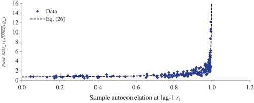
Using URSS as a variable is justified by the theoretical model (Equation (19)). Using r₁ as a variable is based on an assumption that an ensemble discharge time series can be approximated by a first-order autoregressive process, known as AR(1) in statistics, in which r₁ is a controlling factor. This assumption was justified by the fact that most of the transect datasets tested in this study have r₁ > 0.7 (e.g. see Fig. 1).

Figure 1. Data for field RSU_m/ as a function of r₁.

Two fundamental physical units, time t and length ℓ, are involved in the three variables in Equation (21). According to the Buckingham π theorem, these three variables should form one dimensionless group. Since r₁ is dimensionless, the ratio between the square root of var(Q_m) and that of URSS can be written as a function of r₁:

(23)

where g(r₁) is an empirical autocorrelation bias correction factor. Rearranging Equation (23), the proposed semi-empirical model for RSU_m is:

(24)

Comparing the semi-empirical model (Equation (24)) with the theoretical model (Equation (19)), the only difference between the two models is the autocorrelation bias correction factor. For an uncorrelated time series, g(r₁) = 1 and λ_N = 1, the semi-empirical model and the theoretical model are the same.

The empirical autocorrelation bias correction factor g(r₁) in the semi-empirical model needs to be determined using field RSU_m datasets, i.e. the Type A uncertainty estimation for measurements with multiple transects under steady flow conditions. The determination of g(r₁) is called the model calibration. After the calibration, the model should be verified using other field RSU_m datasets than those used in the model calibration.

3 Calibration of the semi-empirical model

The calibration of the semi-empirical model was conducted using Excel spreadsheets. When calibrating the model, we had 205 transect datasets from 36 measurements made with Teledyne RD Instruments ADCPs. For each measurement, we first ran the WinRiver II software to create an ASCII output file of data for cumulated discharge time series (WinRiver II does not output ensemble discharge time series data). The ASCII output file was then imported into an Excel spreadsheet, in which an ensemble discharge time series was calculated from the cumulated discharge time series. The transect discharge summary table for the measurement, generated by WinRiver II, was copied and pasted onto the spreadsheet.

The field RSU_m is assumed to be the approximate true uncertainty of a single transect discharge measurement:

(25)

where s is the sample standard deviation of the transect discharges and is the mean of the transect discharges. The constant c₄ is the bias correction factor for s (e.g. Wadsworth 1989); , where Г(.) stands for the Gamma function; and m is the number of transects in the measurement. It is well known in statistics that is a mean-unbiased estimator of the population standard deviation σ. That is, the expectation of is σ.

It should be pointed out that, for the assumption of the approximate true uncertainty to be valid, the transect discharges used to calculate field RSU_m must be free of directional bias. In general, directional bias in discharge is insignificant and negligible when velocity data are referenced to bottom tracking. When velocity data are referenced to GPS, however, a significant directional bias may occur if the ADCP coordinates are misaligned with the GPS coordinates (e.g. incorrect setting of local magnetic variation) or the ADCP has a heading error. The ADCP misalignment induced directional bias can be corrected in post-processing. The compass (heading) error induced directional bias may be minimized with careful compass calibration prior to measurements at a site. In this study, among the 205 transect datasets used in the model calibration, 149 datasets are referenced to bottom tracking and 56 datasets are referenced to GPS. For the 56 datasets referenced to GPS, directional biases were corrected in data post-processing through the correction of misalignment angles.

The field RSU_m of a measurement was calculated using Equation (25). The sample statistics URSS and r₁ for each transect in the measurement were calculated using Equations (17) and (22), respectively. No spatial averaging (or moving averaging) was applied to ensemble discharge time series when calculating URSS and r₁. The data for the ratio between field RSU_m and as a function of r₁ for the 205 transects are presented in Figure 1.

It can be seen from Figure 1 that the data exhibit a unique relationship between field RSU_m/() and r_1. By trial and error, an empirical equation for g(r₁), which fits the data reasonably well, is constructed as:

(26)

Notice from Figure 1 that field RSU_m/() is as high as 12 for a highly correlated ensemble discharge time series (r₁ is as high as 0.995). The highly correlated ensemble discharge time series were collected on large rivers such as the Mississippi (USA) and Yangtze (China), which is expected because large rivers tend to have a high level of trends and large eddies.

Also notice from Figure 1 that g(r₁) approaches unity when r₁ < 0.8, suggesting that the autocorrelation may be ignored in estimating RSU_m for r₁ < 0.8. Keep in mind that r₁ is calculated from raw ensemble discharge time series without de-trending. Thus, r₁ contains contributions from eddy structures as well as trends. However, a trend that contributes to the autocorrelation may not necessarily contribute to the bias in the estimated RSU_m. Monte Carlo simulations were conducted using a number of synthetic ensemble discharge time series with a trend plus random errors. The results indicate that the uncertainty of the discharge generated from the synthetic ensemble discharge time series is independent of r₁. Note that the estimated r₁ from a synthetic ensemble discharge time series is purely due to the trend because the synthetic ensemble discharge time series cannot mimic eddy structures. In addition, although large rivers tend to have large r₁ values, the r₁ value cannot be predicted from hydraulic conditions at a site; it must be calculated using ensemble discharge time series data.

Moreover, g(r₁) should converge to unity when r₁ approaches zero. However, notice from Equation (26) that g(r₁) is less than unity when r₁ approaches zero. This is because URSS may account for a portion of uncertainties induced by float-swing during a transect. The transect data having low r₁ values were collected in slow flow conditions in which a float had a significant swing. It is known that float-swing may cause a random error that is only significant for measurements in slow flows. Float-swing can be minimized by using a traveler system developed by Willsman (2006).

4 Results of model calibration and verification

Table 1 shows a summary of the site information, the field RSU_m, and the mean of the estimated RSU_m for the 36 measurements used in the model calibration. The estimated RSU_m for each transect in a measurement may not be the same (see the discussion on the model robustness below). The use of the mean of the estimated RSU_m is based on an assumption that all transect discharges in a measurement come from the same transect discharge population; the estimated RSU_m for each transect is an estimate of the transect discharge population standard deviation (relative to the measured discharge). The validation of the IVE method for uncertainty estimation of the current meter method also used the mean of the IVE-estimated uncertainties for multiple measurements at a station (Cohn et al. 2013).

Table 1. Field RSU_m and the mean of estimated RSU_m used in the model calibration.

River and ADCP model	Data collection date (dd/mm/yyyy)	m	Mean Qm (m^3s^−1)	Qedge/Q	Mean Vw (m s^−1)	Mean Vb/Vw	Field RSUm (%)	Mean estimated RSUm (%)
Bei River at Shijiao, China WHR1200, BT	04/12/2009	4	469.7	0.0547	0.7213	1.498	2.700	2.141
Bogburn Stream, New Zealand SP, BT	27/04/2008	4	0.0307	0.0909	0.0758	0.122	2.953	3.383
Choa Praya River, Thailand RR, BT	29/03/2012	4	1877	0.0046	0.6428	1.287	1.070	1.523
Haerbin, China WHR1200, BT	31/08/2010	4	3080	0.0029	0.8308	1.471	1.869	1.706
Haerbin, China WHR1200, GGA	31/08/2010	4	3366	0.0026	0.9068	1.349	0.975	1.846
Haerbin, China WHR1200, BT	15/09/2010	6	3433	0.0013	0.7175	2.037	1.218	1.517
Han River, Korea RiverRay BT	30/05/2013	6	325.7	0.0002	0.1887	4.720	0.910	0.728
Han River, Korea WHR1200, BT	30/05/2013	4	321.6	0.0006	0.1910	4.534	0.970	1.186
Hebei Langfang, China WHR1200, BT	08/12/2011	4	12.92	NA	0.2845	0.616	1.197	2.216
Han River at Hankuo, China WHR600, BT	04/02/2010	4	3732	0.0358	0.9013	2.206	0.902	1.554
Han River at Hankuo, China WHR600, GGA	04/02/2010	4	3784	0.0341	0.9103	2.191	1.805	1.515
Indian Creek at Oveland Park, KS, USA SP, BT	13/05/2003	6	0.360	0.2863	0.1055	0.398	7.588	6.809
Irrigation canal at IID, CA, USA SP, BT	26/08/2003	10	5.709	NA	0.3998	0.176	2.649	2.934
Irrigation canal at IID, CA, USA SP, BT	12/09/2003	5	8.881	0.0177	0.5022	0.145	2.632	4.199
Irrigation canal near Cal Poly, CA, USA SP, BT	06/02/2004	4	1.162	0.0243	0.1850	0.168	3.750	2.683
Irrigation canal at Spruce Weir at IID, CA, USA SP, BT	10/12/2003	7	4.175	0.0135	0.3113	0.435	2.350	2.768
Jiujian River Site 1, China WHR600, GGA	02/07/2007	4	40 947	0.0003	1.4855	0.936	1.050	1.512
Jiujian River Site 2, China WHR600, GGA	02/07/2007	4	40 339	0.0046	1.9838	0.665	2.620	1.685
Kissimmee River, FL, USA WHR600, BT	13/10/2011	4	508.7	0.0028	0.6230	0.620	0.800	0.867
Kissimmee River, FL, USA WHR600, GGA	13/10/2011	4	545.3	0.0028	0.6673	0.614	0.923	0.877
Manilla River, Australia RR, BT	04/12/2013	8	46.61	0.0155	0.7905	0.641	2.600	2.208
Mississippi River, USA WHR600, GGA	15/10/2009	11	15 068	0.0007	1.2114	1.607	1.462	1.482
Mississippi River, USA WHR600, GGA	16/10/2009	12	16 016	0.0018	1.0138	2.077	1.700	1.528
Mississippi River, USA RR, GGA	15/10/2009	9	15 759	0.0004	1.2672	1.536	1.631	1.621
Mississippi River, USA RR, GGA	16/10/2009	8	17 423	0.0015	1.0955	1.895	1.542	1.537
Natural stream, New Zealand NIWA, SP, BT	22/08/2013	4	4.82	0.0109	0.6070	0.063	3.063	3.499
NIWA traveler test, New Zealand SP, BT	03/08/2006	9	0.0347	0.0541	0.0651	0.142	1.488	2.233
San Diego River, CA, USA SP, BT	02/05/2003	7	0.252	0.1555	0.0731	0.471	6.794	7.309
Shanghai Jinhuigang, China WHR600, BT	29/09/2012	6	129.8	0.0095	0.3853	0.957	2.296	1.727
Yangtze River at Three Gorges Reservoir, China WHM300, BT	01/06/2003	3	4697	0.0026	0.1473	9.426	3.840	4.381
Yangtze River at Hankou, China WHR600, BT	02/12/2009	3	8728	0.0559	0.8067	2.123	1.745	0.793
Yangtze River near Three Gorges, China WHM150, BT	19/09/2002	5	11 251	0.0000	0.7952	0.985	1.792	4.358
Yangtze River near Three Gorges, China WHM300, BT	20/09/2002	6	11 400	0.0064	0.8093	1.746	1.272	2.388
Yangtze River near Three Gorges, China WHR600, BT	20/09/2002	3	11 803	0.0138	1.0063	1.487	4.044	3.393
Yunnan Kunming, China RR, BT	19/05/2013	5	1.000	0.0692	0.0328	3.105	11.112	9.985
Yunnan Kunming, China RR, BT	20/05/2013	10	1.200	0.0156	0.0344	3.157	8.162	9.549

RR: RiverRay ADCP model; WHR1200: 1200-kHz Rio Grande ADCP; WHR600: 600-kHz Rio Grande ADCP; SP: StreamPro ADCP; WHM300: 300-kHz Monitor ADCP; WHM150:d 150-kHz Monitor ADCP. BT: bottom tracking; GGA: GGA data of GPS. V_w: channel mean velocity; V_b: boat velocity. IID: Imperial Irrigation District. NA: edge data not available.

It can be seen from Table 1 that the 36 measurements used in the model calibration cover a large range of rivers, flows, and operational conditions. The measured discharge ranges from 0.0307 m³ s⁻¹ on the Bogburn Stream in New Zealand to 40 947 m³ s⁻¹ on the Jiujian River in China. The channel mean velocity ranges from 0.0328 m s⁻¹ on a small stream in Yunnan Kunming, China, to 1.98 m s⁻¹ on the Jiujian River. The ratio between the boat and water velocities ranges from 0.063 on a natural stream in New Zealand to 9.43 on the Yangtze River at the Three Gorges Reservoir in China. These measurements were made with six ADCP models: RiverRay, 1200-kHz Rio Grande, 600-kHz Rio Grande, 300-kHz Monitor, 150-kHz Monitor, and StreamPro ADCPs, operated in Mode 1, Mode 12, Mode 5, or the automatic mode. The size of ADCP depth cells ranged from 2 cm to 2 m and the ensemble time ranged from 0.5 s to 2 s.

After the model was calibrated, we accumulated an additional 382 transect datasets from 48 measurements made with five ADCP models: RiverRay, 1200-kHz Rio Grande, StreamPro, RiverPro, and RioPro ADCPs. These additional datasets, which also cover a large range of rivers, flows, and operational conditions, were used in the model verification. The summary table for the verification datasets is not shown here to save space.

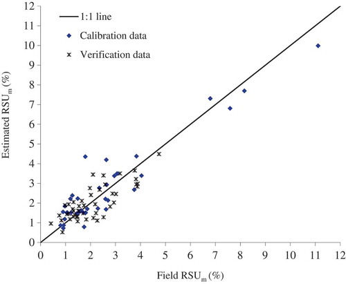
Figure 2 shows a comparison between the field RSU_m and the mean of the estimated RSU_m for the calibration and verification datasets. It can be seen from Figure 2 that the estimated RSU_m for the calibration datasets agrees reasonably well with the field RSU_m. This was expected because the model was calibrated using the calibration datasets. It is encouraging that the estimated RSU_m for the verification datasets also agrees reasonably well with the field RSU_m, which demonstrates the validity of the semi-empirical model.

Figure 2. Comparison between the field RSU_m and the mean of estimated RSU_m.

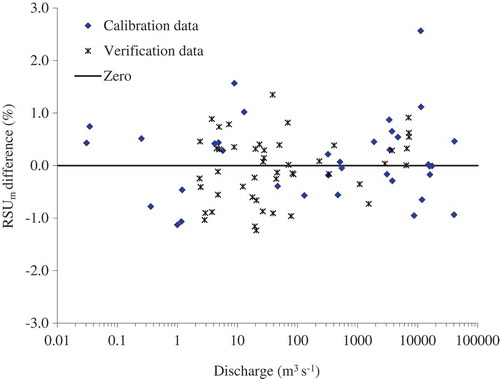
Figure 3 shows the difference between the estimated and field RSU_m as a function of the measured discharge. It can be seen from Figure 3 that the data for the RSU_m difference are randomly distributed around zero; there is neither significant bias (the mean of the RSU_m difference is only 0.025%) nor apparent correlation between the RSU_m difference and the measured discharge. This suggests that the model is independent of the measured discharge, or the size of rivers.

Figure 3. Difference in RSU_m as a function of the measured discharge.

It should be pointed out that a high level of agreement between the estimated and field RSU_m was not expected because the field RSU_m itself has an uncertainty due to the small sample sizes, ranging from 3 to 14 in the calibration datasets and from 4 to 17 in the verification datasets. It is known that the Type A uncertainty estimated from small samples has uncertainty (JCGM 2008, Huang 2014). However, it was expected that the level of agreement would be high for large samples and low for small samples. To examine this, we divided the total 84 measurements into two groups: Group A having 48 measurements with sample size less than 8 and Group B having 36 measurements with sample size equal or greater than 8. The mean of the RSU_m difference is 0.114% for Group A and −0.095% for Group B; the standard deviation is 0.755% for Group A and 0.568% for Group B. Apparently, Group B has less variance than Group A. From this result we may infer that the estimated RSU_m is more accurate than the field RSU_m for small samples. Tests with additional large samples are needed to verify this inference. If verified, the estimated RSU_m may be more appropriate than the field RSU_m for uncertainty analysis and uncertainty-based measurement quality control, because in practice most of measurements may consist of a small number of transects (typically four). Readers may refer to Huang (2014, 2015) for detailed information on the uncertainty-based measurement quality control.

5 Discussion

5.1 Two-point and five-point based estimators

The semi-empirical model employs the three-point based estimator in the calculation of URSS. It was of interest to see what the result would be if other estimators, such as a two-point or five-point based estimator, were used. To address this concern, we tested a two-point based estimator and a five-point based estimator . Notice that either estimator is a moving-average. The estimator bias correction factor for each of the two estimators is derived following the same approach to deriving the estimator bias correction factor for the three-point based estimator. The results are for the two-point based estimator and for the five-point based estimator.

For an uncorrelated, stationary time series, URSS is independent of the number of points used in an estimator. We tested the two-, three- and five-point based estimators through Monte Carlo simulation with randomly generated numbers that are uncorrelated and stationary. The results for URSS from the three estimators were nearly identical (only having very small numerical variance). We also tested the three estimators with several ensemble discharge time series. The results for URSS from the two-point and five-point based estimators were not significantly different from those from the three-point based estimator. Taking the dataset of the irrigation canal near Cal Poly as an example, the square root of URSS was 0.03101, 0.02707, and 0.2996 for the two-, three-, and five-point based estimators, respectively. Recall that an ensemble discharge time series is neither uncorrelated nor stationary. Therefore, it is expected that the calculated URSS may vary slightly with the number of points used in an estimator. However, this would not be a problem because the calibration of the semi-empirical model has accounted for the number of points used in estimators.

5.2 Robustness of the semi-empirical model

In addition to the model calibration and verification, the performance of the semi-empirical model was evaluated for its robustness. It is very common that the transects in a measurement have some differences in the number of ensembles, boat speed, and the boat’s track. The robustness is the consistency in the estimated uncertainties for different transects in a measurement; it is measured by the percentage difference between the estimated RSU_m of a transect and the mean of the estimated RSU_m (denoted by ) of all transects in the measurement:

(27)

We calculated PD for the 205 transects used in the model calibration. The histogram (not shown here) of the PD data is approximately bell-shaped. The mean of the PD values is zero; the standard deviation is 13.64%. Thus, on average, the estimated RSU_m of a transect should be within ±27.28% of the mean of the estimated RSU_m of all transects in a measurement, at the 95% confidence level. This suggests that the semi-empirical model is robust, i.e. it is not significantly sensitive to differences in transects of a measurement.

5.3 Correction for bias due to negative ensemble discharge

It is not uncommon that an ensemble discharge time series contains negative values. Negative ensemble discharges can be caused by backward-tracks or back-flows. The ADCP discharge calculation algorithm accounts for negative ensemble discharges. It is well known that an ADCP discharge measurement is track independent, i.e. it is independent of the shape of the boat track. This has been verified by some ADCP users who intentionally made different track configurations, such as S-shaped, arch-shaped, or even having a loop in the middle of a track. However, the estimated RSU_m will be positively biased if an ensemble discharge time series contains negative values. To understand this, consider an extreme case where a transect is made with a loop in the middle of the track. The positive and negative ensemble discharges associated with the loop are cancelled, so that the loop has no contribution to Q_m. That is, Q_m would be the same regardless of whether the track was looped or straight. However, as seen in Equation (18), URSS is the sum of all squared ensemble discharge residuals, regardless of whether an ensemble discharge is positive or negative. Therefore, the calculated URSS associated with a looped track will be greater than that associated with a straight track; the estimated RSU_m will be higher than it should be.

To correct the bias due to negative ensemble discharges, we introduce a bias correction factor, denoted by k:

(28)

where Q′_m is the sum of the absolute ensemble discharges. Since Q′_m ≥ Q_m (0 < k ≤ 1), the estimated uncertainty with the bias correction, RSU′_m, is calculated as:

(29)

As an example of the bias correction, Table 2 shows a comparison between the estimated RSU_m and RSU′_m for the transect discharges measured on the Aksu River in Turkey on 21 February 2011 using a StreamPro ADCP. The boat tracks of the first four transects were relatively straight, while the boat track of the fifth transect was intentionally made to have a loop in the middle of the track.

Table 2. Comparison between the estimated RSU_m and RSU′_m.

Transect data file	Qm (m^3 s^−1)	k	RSUm (%)	RSU′m (%)	Track
Aksu_River_SP000	37.284	0.9659	3.52	3.40	Straight
Aksu_River_SP001	37.934	0.9590	3.66	3.51	Straight
Aksu_River_SP002	37.930	0.9686	3.18	3.08	Straight
Aksu_River_SP003	38.304	0.9890	3.62	3.58	Straight
Aksu_River_SP004	36.422	0.4547	7.17	3.26	Looped

It can be seen from Table 2 that the Q_m of the fifth transect is consistent with that of the first four, but its RSU_m is 7.17%, significantly greater than that of the first four transects. After bias correction, the RSU′_m of the fifth transect becomes 3.26%, which is consistent with the first four transects.

It should be pointed out that the above bias correction is applicable only to negative ensemble discharges induced by backward-tracks or back-flows. It should not be used for negative ensemble discharges induced by noisy velocity measurements. Noisy velocity data are commonly collected in extreme low-flow conditions (e.g. velocity of the order of 5 cm s⁻¹), which can be easily identified from a plot of velocity sticks on a boat track. A number of transects were made under extreme low-flow conditions and the estimated RSU_m was found to be reasonable without the bias correction for negative ensemble discharges due to noisy velocity measurements.

5.4 Missing ensembles

It is also not uncommon that ADCP data contain missing ensembles. In discharge calculation, the missing ensemble discharges are accounted for by the next valid velocity cross-product multiplied by the cumulated time of the missing ensembles (TRDI 2009). Thus, the missing ensembles have zero discharge values and the next valid ensemble has a lumped discharge value, which results in spikes in ensemble discharge time series.

Missing ensembles may induce errors in estimation of URSS and r₁. To minimize potential errors, a lumped discharge is uniformly distributed over the missing ensembles; this is known as back-extrapolation. The back-extrapolation method was tested for a number of transects. The results for a transect in the Mississippi River ADCP discharge measurement on 10 October 2009 are presented here for discussion. This transect has a total of 745 ensembles, with 25 ensembles missing. The measured discharge is 15 190 m³ s⁻¹. The square root of URSS is 96.06 m³ s⁻¹ and r₁ is 0.9639 for the ensemble discharge time series with spikes; the estimated RSU_m is 1.392%. The back-extrapolation was applied on the missing ensembles, which made no change in the measured discharge. The square root of URSS now is 37.98 m³ s⁻¹ and r₁ is 0.9919; the estimated RSU_m is 1.330%. Assume that the URSS and r₁ estimated with the missing ensemble correction are the true values. The spikes caused a positive bias in the estimated URSS and a negative bias in the estimated r₁. However, it is interesting to note that the relative difference between the estimated RSU_m with and without the missing ensemble correction is insignificant, only 4.6%. This result (also similar results from other transects tested) seems to suggest that the semi-empirical model is not significantly sensitive to missing ensembles. However, we suggest conducting the back-extrapolation prior to calculating URSS and r₁. This is because the spikes are not the “real” spikes. Back-extrapolation may be considered to be a reasonable approach to dealing with missing data. However, back-extrapolation may be applicable only when the missing ensembles are an insignificant portion of the total ensembles. A missing ensemble itself is a data quality issue. A transect with a significant amount of missing ensembles may not be qualified as a valid measurement.

5.5 Uncertainty with contribution of edges

The uncertainty RSU including the contribution of edges can be estimated using Equation (2). To examine the contribution of edges, the data for the ratio between the estimated RSU and the estimated RSU_m (RSU/RSU_m) are presented as a function of the ratio between the edge discharge and the total discharge (Q_edge/Q) (Fig. 4). It can be seen from Figure 4 that the ratio RSU/RSU_m is around 1 (with only one outlier) for Q_edge/Q < 0.05 (or 5%). This is expected, because, when the edge discharge is small relative to the total discharge (say, <5%), its contribution to the uncertainty should be small. Notice that the RSU/RSU_m ratio may not always be >1; it could be slightly smaller than 1. Although the absolute uncertainty with the edge contribution would be greater than the absolute uncertainty without it, RSU could be smaller than RSU_m because the denominator Q in RSU is usually greater than the denominator Q_m in RSU_m, which sometimes compensates for the increase in the absolute uncertainty with contributions of edges.

Figure 4. Ratio RSU/RSU_m as a function of Q_edge/Q.

In contrast, the field RSU can be calculated using the transect datasets for the total discharge including edge discharges (i.e. use Q to replace Q_m in Equation (25)). We compared the estimated RSU with the field RSU for the calibration and verification datasets except for two datasets that had no edge data (edge distances were set to zero). Figure 5 shows the relative difference between the estimated RSU and the field RSU as a function of Q_edge/Q. It can be seen from Figure 5 that most of the data for the RSU difference (%) are within ±1.3% except for two data points. These two outliers correspond to the two low-flow cases where Q_edge/Q is relatively large. One case has Q = 0.360 m³ s⁻¹ and Q_edge/Q = 0.29, while the other has Q = 0.252 m³ s⁻¹ and Q_edge/Q = 0.16. Figure 5 indicates that the agreement between the estimated and field RSU is reasonably good and is compatible with the agreement between the estimated and field RSU_m for Q_edge/Q < 0.1. The mean and standard deviation of the RSU difference are 0.002% and 0.638%, respectively (excluding the two outliers), whereas those of the RSU_m difference are 0.025% and 0.685%, respectively (all data). Thus, Equation (2) is valid for estimating the uncertainty RSU with an edge contribution. However, if the flow is very low and Q_edge/Q is relatively large (say, >0.15), according to the limited test results (i.e. the two data points), the RSU model (Equation (2)) may overestimate the uncertainty.

Figure 5. Difference in RSU as a function of Q_edge/Q.

5.6 Comparison between WinRiver II and QRev calculated discharges

As mentioned in Section 1, Mueller (2016a, 2016b) developed a computer program named QRev, which automates filtering and quality checking of the collected data. Importantly, QRev employs the US Geological Survey (USGS) standard algorithms for discharge calculation. That is, QRev applies the same algorithms to data independent of manufacturer of the ADCP used to collect the data. The mathematical formulation for discharge calculation in both WinRiver II and QRev is the same. However, according to Mueller (2016b), a major difference between the two programs is the algorithms to estimate values for invalid data. WinRiver II essentially employs backward propagation of data, while QRev employs linear interpolations. Recall that all data used in this study were collected with Teledyne RD Instruments ADCPs, and the discharges were calculated with WinRiver II (Version 2.18). A concern was raised about whether the discharges calculated with WinRiver II would agree with the discharges calculated with QRev. A comprehensive comparison between WinRiver II and QRev calculated discharges is beyond the scope of this study and the present paper. However, to gain confidence in the calculated discharges with WinRiver II, we used QRev (Version 3.21) and calculated the measured discharges for the first 10 datasets shown in Table 1. In the comparison calculations, both WinRiver II and QRev used the 1/6 power law for velocity extrapolations and all other user settings were also the same. Table 3 shows the results for the relative difference (in percentage) between the WinRiver II and QRev calculated discharges. The percentages of invalid (bad) ensembles and bins, which were the outputs from WinRiver II, are also shown in Table 3.

Table 3. Relative difference between the WinRiver II calculated discharge and the QRev calculated discharge for the first 10 datasets shown in Table 1.

River and ADCP model	WinRiver II discharge	QRev discharge	Difference	Invalid ensembles	Invalid bins
	(m^3 s^−1)	(m^3 s^−1)	(%)	(%)	(%)
Bei River Shijiao, China; WHR1200, BT	496.936	498.119	−0.237	7	0
Bogburn stream, New Zealand; SP, BT	0.033	0.032	3.125	2	19
Choa Praya River, Thailand; RR, BT	1886.011	1886.780	−0.041	0	1
Haerbin, China; WHR1200, BT	3088.575	3084.610	0.129	1	0
Haerbin, China; WHR1200, GGA	3374.786	3372.405	0.071	0	0
Haerbin, China; WHR1200, BT	3437.626	3438.95	−0.039	0	0
Han River, Korea; RiverRay, BT	325.735	326.497	−0.233	1	1
Han River, Korea; WHR1200, BT	321.812	321.763	0.015	4	0
Hebei Langfang, China; WHR1200, BT	12.925	12.926	−0.008	0	0
HK, China; WHR600, BT	3870.851	3827.989	1.120	7	0

It can be seen from Table 3 that most of the differences are very small. The largest difference (3.125%) is largely due to the fact that the measured discharge is extremely small and the outputs from WinRiver II and QRev have only two significant figures. Notice that this measurement has 19% invalid bins, which may also contribute to the difference in the calculated discharges. Excluding the outlier (3.125%), the mean difference is only 0.086%. Thus, the results from this comparison indicate that the WinRiver II and QRev calculated discharges agree very well. However, further investigation is needed to evaluate the performance of the two software packages.

It should be pointed out that, in principle, the difference between the WinRiver II and QRev calculated discharges is considered as the relative “bias,” not random error. This is because, for a given transect data, the difference between the calculated discharges is a “constant.” By definition, the random uncertainty is independent of the “true” value or bias. In other words, the random uncertainty is independent of discharge calculation algorithms. Thus, the random uncertainty model presented in this paper is also applicable to the QRev calculated discharges.

6 Conclusions

The theoretical model presented explores the theoretical relationships between the variables involved in the problem. It was tested with a number of transect datasets with mixed results. The performance of the theoretical model depends on the accuracy of the estimated theoretical autocorrelation bias correction factor λ_N from ensemble discharge time series.

The presented semi-empirical model is essentially a Type A model based on statistical analyses of ensemble discharge time series. The model was calibrated with 205 transect datasets from 36 measurements; it was verified with an additional 382 transect datasets from 48 measurements. The calibration and verification datasets cover a large range of rivers, flows, and operational conditions. The robustness of the model was also verified.

One of the advantages of the semi-empirical model is that it accounts for site-specific conditions and all random error sources in discharge measurement. This is because the two sample statistics URSS and r₁ in the semi-empirical model are obtained by statistical analysis of ADCP ensemble discharge time series data collected at a site. The site-specific data contain effects induced by all random error sources, including ADCP system noise in velocity and depth measurements, ambient turbulence, random errors and/or variations of pitch, roll, heading, temperature, and ADCP draft. In addition, the random error in distance to the edge is accounted for by a Type B uncertainty component in the RSU model.

The presented semi-empirical model is applicable to any ADCP, regardless of manufacturer or model. It is independent of system configurations and user settings. The model can be implemented in an Excel spreadsheet or a computer program. It provides a useful tool for uncertainty analysis and uncertainty-based measurement quality control of moving-boat ADCP streamflow measurements. The model has recently been implemented in Q-View (TRDI 2015), a software system for quality assessment of moving-boat streamflow measurements made with Teledyne RD Instruments ADCPs.

Acknowledgements

The author would like to thank Timothy Cohn, Julie Kiang, David Mueller, Kevin Oberg, and Thomas Over of the US Geological Survey, who reviewed the two early versions of this paper and provided helpful comments. The majority of the ADCP data used in this study were collected or provided by other people. To mention only a few: Andrew Willsman of the National Institute of Water and Atmospheric Research, New Zealand; Jeffrey Den Herder, Ian Cassimatis, Zhanping Xi, and Loic Michel of Teledyne RD Instruments. The author would also like to thank the anonymous reviewers for their valuable comments that helped improve the quality of this paper.

Disclosure statement

No potential conflict of interest was reported by the author.

Appendix 1: Variance and uncertainty of edge discharges

 

The edge discharge may be estimated as (e.g. TRDI 2009):

(A1)

where Q_e is the edge discharge (either right or left edge), C is the edge coefficient (0.3535 for triangular and 0.91 for rectangular shape), L_e is the edge distance measured from a bank to the first or last ensemble location, d_e is the mean depth of the edge ensembles, and V_e is the mean velocity magnitude of valid cells in the edge ensembles.

We assume that L_e, d_e, and V_e are independent random variables. The edge distance L_e is measured by a means other than an ADCP. It is entered into the ADCP operation software by the operator at the beginning and the end of a transect. Therefore, L_e is independent of d_e and V_e, which are measured by the ADCP. The ADCP depth and velocity measurements can be assumed independent because the bottom tracking pulse and the water tracking pulse are separate pulses.

The variance of the edge discharge Q_e can be estimated as:

(A2)

where var (d_eV_e) is the variance of the product of the edge depth and velocity. It can be estimated using the edge ensemble data for depth and velocity:

(A3)

where is the mean of the product, and N_e is the number of edge ensembles (default 10 in the WinRiver II software).

If RSU_e is denoted as the relative standard uncertainty of the edge discharge, RSU_e can be estimated as:

(A4)

where u_L is the relative standard uncertainty in width measurement:

(A5)

The u_L can be estimated as a Type B uncertainty using the values presented in Table E.1 in ISO 748 (2007).

Appendix 2: Derivation of the estimator bias correction factor

 

Equation (14) is rewritten here:

(A6)

The ensemble discharge residual ∆q_i is also rewritten here:

(A7)

The mean of ∆q_i is zero for the estimator used. Thus, Equation (A6) can be rewritten as:

(A8)

Substituting the three-point based estimator (Equation (15)) into Equation (A7), and rearranging, yields:

(A9)

Taking variance on both sides of Equation (A9) yields:

(A10)

Assume that the variances of the ensemble discharge at i – 1, i, and i + 1 are identical. Equation (A10) can be reduced to:

(A11)

Comparing Equation (A11) with Equation (A8), the estimator bias correction factor for the three-point based estimator is determined as .

References

- Boldt, J.A. and Oberg, K., 2015. Validation of streamflow measurements made with M9 and RiverRay acoustic Doppler current profilers. Journal of Hydraulic Engineering. doi:10.1061/(ASCE)HY.1943–7900.0001087
- Christensen, J.L. and Herrick, L.E., 1982. Mississippi river test: volume 1: final report. DCP4400/300, prepared for the US Geological Survey by AMETEK/Straza Division, El Cajon, California, under contract no. 14-08-0001-19003.
- Cohn, T., Kiang, J., and Mason Jr., R., 2013. Estimating discharge measurement uncertainty using the interpolated variance estimator. Journal of Hydraulic Engineering, 139 (5), 502–510. doi:10.1061/(ASCE)HY.1943-7900.0000695
- EC (Environment Canada), 2004. Procedures for the review and approval of ADCP discharge measurements. 1st ed. Ottawa, Canada: Environment Canada.
- García, C., et al., 2012. Variance of discharge estimates sampled using acoustic Doppler current profilers from moving platforms. Journal of Hydraulic Engineering, 138 (8), 684–694. doi:10.1061/(ASCE)HY.1943-7900.0000558
- González-Castro, J.A., Buzard, J., and Mohamed, A., 2016. RiverFlowUA—a package to estimate total uncertainty in ADCP discharge measurements by FOTSE—with an application in hydrometry. In: G. Constantinescu, M. Garcia, and D. Hanes, eds. River Flow 2016 (Proceedings of the Eighth International Conference on Fluvial Hydraulics, 12–15 July 2016, St. Louis, MO. London: Taylor & Francis Group, 715–723.
- González-Castro, J.A. and Muste, M., 2007. Framework for estimating uncertainty of ADCP measurements from a moving boat by standardized uncertainty analysis. Journal of Hydraulic Engineering, 133 (12), 1390–1410. doi:10.1061/(ASCE)0733-9429(2007)133:12(1390)
- Huang, H., 2006. Analysis of random error in ADCP discharge measurement, Part I: a model for predicting random uncertainty. China Journal of Hydraulic Engineering, 37 (5), 619–624. (in Chinese).
- Huang, H., 2008. Estimating precision of moving boat ADCP discharge measurement. In: Proceedings (DVD) of 14th Australian hydrographers association conference: water initiatives 2008 and beyond. Northcote: Australia Hydrographers Association.
- Huang, H., 2012. Uncertainty model for in situ quality control of stationary ADCP open channel discharge measurement. Journal of Hydraulic Engineering, 138 (1), 4–12. doi:10.1061/(ASCE)HY.1943-7900.0000492
- Huang, H., 2013. Closure to “Uncertainty model for in situ quality control of stationary ADCP open-channel discharge measurement” by Hening Huang. Journal of Hydraulic Engineering, 139 (1), 104–106. doi:10.1061/(ASCE)HY.1943-7900.0000667
- Huang, H., 2014. Uncertainty-based measurement quality control. Accreditation and Quality Assurance, 19 (2), 65–73. doi:10.1007/s00769-013-1032-5
- Huang, H., 2015. Statistical quality control of streamflow measurements with moving-boat acoustic Doppler current profilers. Journal of Hydraulic Research, 53 (6), 820–827. doi:10.1080/00221686.2015.1074947
- Huang, H., 2016. Estimation of Type A uncertainty of moving-boat ADCP streamflow measurements. In: I.G. Constantinescu, M. Garcia, and D. Hanes, eds. River Flow 2016 (Proceedings of the Eighth International Conference on Fluvial Hydraulics, 12–15 July 2016, St. Louis, MO. London: Taylor & Francis Group, 696–701.
- ISO 5168, 2005. Measurement of fluid flow – procedures for the evaluation of uncertainties. Geneva, Switzerland: International Organization for Standardization.
- ISO 748, 2007. Hydrometry – measurement of liquid flow in open channels using current meters or floats. Geneva, Switzerland: International Organization for Standardization.
- Joint Committee for Guides in Metrology (JCGM), 2008. Evaluation of measurement data - Guide to the expression of uncertainty in measurement (GUM 1995 with minor corrections). Geneva, Switzerland. Available from: http://www.bipm.org/utils/common/documents/jcgm/JCGM_100_2008_E.pdf.
- Law, A.M. and Kelton, W.D., 1991. Simulation modeling and analysis, 2nd ensemble discharge. New York: McGraw-Hill.
- Moore, S.A., et al., 2017. Monte Carlo approach for uncertainty analysis of acoustic Doppler current profiler discharge measurement by moving boat. Journal of Hydraulic Engineering, 143 (3), 04016088. doi:10.1061/(ASCE)HY.1943-7900.0001249
- Mueller, D.S., 2013. Extrap: software to assist the selection of extrapolation methods for moving-boat ADCP streamflow measurements. Computers & Geosciences, 54, 211–218. doi:10.1016/j.cageo.2013.02.001
- Mueller, D.S., 2016a. QRev: software for computation and quality assurance of acoustic Doppler current profiler moving-boat streamflow measurements – users manual, Version 2.8. Reston, VA: US Geological Survey Report Series 2016–1052.
- Mueller, D.S., 2016b. Consistent and efficient processing of ADCP streamflow measurements. In: G. Constantinescu, M. Garcia, and D. Hanes, eds. River Flow 2016, Proceedings of the Eighth International Conference on Fluvial Hydraulics, 12–15 July 2016, St. Louis, MO. London: Taylor & Francis Group, 655–663.
- Mueller, D.S. and Wagner, C.R., 2007. Correcting acoustic Doppler current profiler discharge measurements biased by sediment transport. Journal of Hydraulic Engineering, 133 (12), 1329–1336. doi:10.1061/(ASCE)0733-9429(2007)133:12(1329)
- Mueller, D.S., et al., 2013. Measuring discharge with acoustic Doppler current profilers from a moving boat. Reston, VA: US Geological Survey Techniques and Methods 3-A22, Version 2.0.
- MWR (Ministry of Water Resources, People’s Republic of China), 2006. Guidance for streamflow measurements using acoustic Doppler current profiler. Beijing, China, SL337-2006.
- Oberg, K.A. and Mueller, D.S., 2007. Validation of streamflow measurements made with acoustic Doppler current profilers. Journal of Hydraulic Engineering, 133 (12), 1421–1432. doi:10.1061/(ASCE)0733-9429(2007)133:12(1421)
- Rennie, C.D. and Rainville, F., 2006. Case study of precision of GPS differential correction strategies: influence on aDcp velocity and discharge estimates. Journal of Hydraulic Engineering, 132 (3), 225–234. doi:10.1061/(ASCE)0733-9429(2006)132:3(225)
- Simpson, M.R., 2001. Discharge measurements using a broad-band acoustic Doppler current profiler. Reston, VA, USA, US Geological Survey Open-File Report 01–1.
- Tarrab, L., et al., 2012. Role of turbulence fluctuations on uncertainties of acoustic Doppler current profiler discharge measurements. Water Resources Research, 48 (6), W06507. doi:10.1029/2011WR011185
- TRDI (Teledyne RD Instruments), 2009. WinRiver II user’s guide. California: Poway.
- TRDI (Teledyne RD Instruments), 2015. Q-view user’s guide. California: Poway.
- USGS (US Geological Survey), 2002. Policy and technical guidance on discharge measurements using acoustic Doppler current profilers. US Geological Survey, Office of Surface Water Technical Memorandum 2002.02 Available from: http://hydroacoustics.usgs.gov/memos/OSW2002-02.pdf [Accessed 13 August 2008].
- Wadsworth Jr., H.M., 1989. Summarization and interpretation of data. In: M. Harrison and H.M. Wadsworth Jr., eds. Handbook of statistical methods for engineers and scientists, ensemble discharges. New York: McGraw-Hill.
- Wagner, C.R. and Mueller, D.S., 2011. Comparison of bottom-track to global positioning system referenced discharges measured using an acoustic Doppler current profiler. Journal of Hydrology, 401 (3–4), 250–258. doi:10.1016/j.jhydrol.2011.02.025
- Willsman, A., 2006. A case study of low flow measurement in a small channel using StreamPro with a customer-made traveler system. In: National Institute of Water and Atmospheric Research, ed. Customer’s success story. New Zealand: National Institute of Water and Atmospheric Research.