Climate change impact assessment of a river basin using CMIP5 climate models and the VIC hydrological model

ABSTRACT

Climate change has significant impacts on water availability in larger river basins. The present study evaluates the possible impacts of projected future daily rainfall (2011–2099) on the hydrology of a major river basin in peninsular India, the Godavari River Basin, (GRB), under RCP4.5 and RCP8.5 scenarios. The study highlights a criteria-based approach for selecting the CMIP5 GCMs, based on their fidelity in simulating the Indian Summer Monsoon rainfall. The nonparametric kernel regression based statistical downscaling model is employed to project future daily rainfall and the variable infiltration capacity (VIC) macroscale hydrological model is used for hydrological simulations. The results indicate an increase in future rainfall without significant change in the spatial pattern of hydrological variables in the GRB. The climate-change-induced projected hydrological changes provide a crucial input to define water resource policies in the GRB. This methodology can be adopted for the climate change impacts assessment of larger river basins worldwide.

KEYWORDS:

• climate change
• Godavari River Basin
• variable infiltration capacity (VIC) model
• statistical downscaling model

Editor A. Castellarin Associate editor J. Thompson

1 Introduction

The impacts of global warming on the hydrological cycle and water resource systems have been an important concern worldwide in recent years. Various general circulation model (GCM) based simulations, studies and experiments have projected an increase in temperature due to the enhanced levels of greenhouse gases. Consequently, climate processes are expected to intensify, leading to severe impacts on agricultural and energy production, ecosystems, water availability, heat waves, waterlogging, flooding and drought. However, these climate-change-driven impacts have regional variations because of the local climate and geographical characteristics; thus, hydrological responses to climate change depend on the regional physical processes (Hay et al. 2011). The projected climate change would certainly affect the hydrology (Dionysia 1992, Baldassarre et al. 2011, Jaewon et al. 2017), long-term water availability (Yu and Wang 2009) and quality (Rehana and Mujumdar 2011) in river basins. The hydrological impacts of climate change are very important and enable water resource managers to make robust decisions on future policy adaptations (Fowler et al. 2007). Several studies have evaluated the impacts of regional climate change on hydrology worldwide, such as in Australia (Chiew and McMahon, 1993), India (Kishtawal et al. 2009, Deshpande et al. 2016), Kenya (Githui et al. 2009) and China (Xu et al. 2011). Regional hydrological responses to global climate change at the river-basin scale have serious implications on socio-economic changes, and must be urgently evaluated to determine socio-economic development and define basin management policies.

Indian river basins receive more than 80% of the total rainfall from the Indian summer monsoon rainfall (ISMR), which occurs during four months, June–September (JJAS) (Webster et al. 1998, Menon et al. 2013). The ISMR is highly complex and exhibits spatial and temporal variability during JJAS (Goswami 2011). The strong sensitivity of the Asian monsoon to global warming aggravates changes in the monsoon precipitation intensity and total monsoon precipitation (Kitoh et al. 2013). The potential consequences of the complexity and severity of the ISMR under changing climate critically affects the water resource systems, ecosystems, agricultural production and socioeconomic situation in the Indian subcontinent (Gadgil and Rupa Kumar 2006). Therefore, accurate projections of the ISMR are extremely important because it is one of the most important drivers for climate change policies and adaptation for Indian river basins.

General circulation models are climate models that account for the long-term effects of greenhouse gases and use mathematical equations representing the physical processes in the atmosphere, ocean and land surface. The models project future climate variables at daily and monthly time scales at a very coarse spatial resolution. They are the most credible available climate models to project the future climate but are not well suited for regional hydrological assessment (Xu 1999, Salvi et al. 2013). Thompson et al. (2016) have reported considerable GCM-related uncertainty and its impact on floods under changing climate. The GCMs often fail to simulate the processes at a finer scale accurately. The accuracy of GCMs decreases at finer resolutions, whereas that of hydrological assessment studies increases at higher resolutions (Xu 1999). Hence, GCM outcomes cannot be used directly in regional hydrological assessment studies. The hydrological assessment is typically carried out at the catchment or river-basin scale by calibrating and validating the hydrological model using the observed streamflow at the outlet. Hence, it is extremely important to bridge the gaps between the coarse-resolution GCMs and fine-resolution hydrological models to evaluate the impact of climate change on the regional hydrology of major catchments or river basins. The methods that convert GCM outputs into local hydrological variables are suitable for hydrological models and are known as downscaling techniques (Dibike and Coulibaly 2007). Two types of downscaling approach may be used: (1) dynamic downscaling techniques to generate high-resolution meteorological variables as per the requirement of the hydrological model; and (2) statistical downscaling to simulate fine-resolution and local-scale surface variables from GCMs, and adopting the macroscale hydrological modelling approach for further hydrological assessments.

Statistical downscaling, a data-driven technique, substantially reduces the computational resources and can be used at the region of interest if sufficient data are available to build the statistical model. Statistical downscaling methods use the established system relationships obtained from the observed data (Hewitson and Crane 1996). Statistical models transform GCM-simulated large-scale climate variables into regional/local-scale climate and hydrological variables (predictands), for example rainfall. In statistical downscaling, the regional climate is assumed to be conditioned by large-scale climate variables and regional physical processes (Dobler and Ahrens 2011, Kannan and Ghosh 2013). Statistical downscaling techniques have been used extensively in regional studies worldwide. Detailed reviews of the downscaling techniques, advantages, limitations and recent developments have been reported by Maraun et al. (2010) and Schoof (2013).

Kling and Gupta (2009) explored the impact of sub-basin-scale variability in the input and parameter for lumped watersheds. The noise in results is observed because of neglecting the spatial variability in physical properties and system complexity. The microscale catchment models are not suitable for larger basins because they may not simulate the scale-dependent hydrological processes in such basins (Dunn 1998). Macroscale hydrological models (MHMs) are developed to assess the climate change impacts on the basin hydrology. A spatially distributed variable infiltration capacity (VIC) model, a MHM, is an excellent tool for assessing climate change impact on water resources at the river basin, regional and continental scales (Hamlet and Lettenmaier 1999, Nijssen et al. 2000, 2001, Maurer et al. 2002, Cuo et al. 2013). The VIC model is developed for incorporation in GCMs and to simulate the hydrological processes at fine spatial resolutions.

The present study aims to assess the impact of the future projected daily rainfall on the hydrology of a major river basin in India, the Godavari River Basin (GRB). Deshpande et al. (2016) evaluated temporal changes in the extreme rainfall (1951–2014) and temperature (1951–2013) for major river basins in India including the GRB. Das and Umamahesh (2016) evaluated the climate change impact on the GRB by projecting the monthly monsoon precipitation for different scenarios using fuzzy clustering with a multiple regression technique. Hengade and Eldho (2016) adopted the VIC model to evaluate the hydrological implications of land-cover changes and rainfall trends in the Ashti catchment (50 990 km²), a sub-basin of the GRB, for a period of 40 years (1971–2010) using the trend analysis method. Shah and Mishra (2016) calibrated and evaluated the VIC model for major river basins in India including the GRB. The above-mentioned studies to assess the impact of climate change on GRB were carried out either for a historical period or at the monthly scale using a single GCM without adopting judicious criteria for selection of GCMs. Earlier studies at the GRB were restricted to rainfall projections. To date, the water balance components have not been evaluated at the daily scale for a period of 90 years (2011–2100).

Most of the CMIP5 GCMs failed to simulate the decreasing trend of the ISMR (Saha et al. 2014). The CMIP5 GCMs were selected based on previously reported judicious criteria (Saha et al. 2014, Sharmila et al. 2015), which evaluated the performance of the model based on its fidelity in simulating a decreasing trend, variability and basic characteristics of the ISMR. Considering these criteria, CNRM-CM5, MIROC-ESM, INM-CM4 and NorESM1-M GCM models are adopted for projecting the future daily rainfall. Firstly, a spatially distributed macroscale hydrological model, the VIC model, was established in the study area. The VIC model is calibrated and validated by comparing the observed and model-simulated streamflow to evaluate the model performance. The kernel regression-based statistical downscaling model is adopted to develop the statistical relationship between the predictor (large-scale reanalysis data) and predictands (fine-scale observed rainfall), and the relationship is then applied to GCM-simulated outputs. The statistical downscaling model is trained on 15 years (1971–1990) of data, validated on 20 years (1991–2005) and further used to project the future rainfall for 90 years (2011–2100) in the GRB. The projected future daily rainfall is incorporated in the VIC model to assess the impacts of climate change in the GRB. This study evaluates the changes in the simulated surface runoff, evapotranspiration and baseflow in the study area between the present and future climate scenarios.

2 Study area description

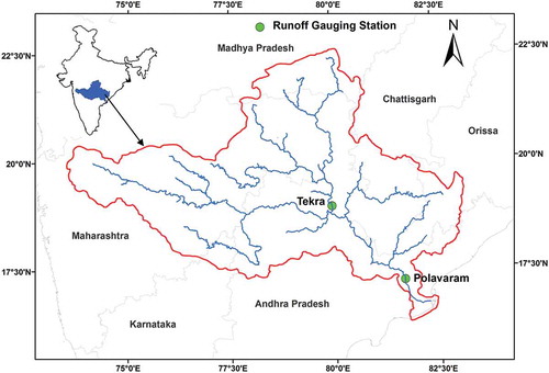
The Godavari, a perennial river and the second largest river basin in India, is situated in the Deccan Plateau. It extends between the longitudes 73°21′–83°09′E and latitudes 16°07′–22°50′N. It covers a catchment area of 312 800 km², accounting for approximately 9.5% of the geographical area of India. Figure 1 shows the geographical setting of the basin. The GRB is bounded by the Eastern Ghats in the east; the Western Ghats, including the Sahyadri ranges in the west; the Ajanta range and Mahadeo hills in the south; and the Satmala hills in the north. The Godavari River originates at Trimbakeshwar in the Nashik District of Maharashtra at an altitude of 1067 m a.s.l. and joins the Bay of Bengal after approximately 1465 km. The major tributaries of the Godavari River are Pranhita, Sabri, Purna, Pravara, Manjra, Maner and Indravati. The GRB extends into major parts of the states of Maharashtra (48.5%), Andhra Pradesh (23.3%) and Chhattisgarh (12.5%), in addition to smaller parts of Madhya Pradesh (8.6%), Orissa (5.7%) and Karnataka (1.4%). The basin is dominated by clay and sandy clay loam, accounting for low infiltration and high runoff. The major part of the GRB covers grassland and cropland areas (60.65%) and woodland (29.37%). The average annual rainfall in the GRB is 1100 mm, which varies temporarily and spatially across the basin. The GRB receives more than 80% of the annual rainfall from the ISMR during JJAS. The spatial variation of the rainfall is significant because some parts of the basin receive 600 mm, whereas other parts receive 3000 mm of annual rainfall. The temperature varies from 18 to 35°C, which causes significant monthly variations in the potential evapotranspiration (PET). The PET is low during January–February and high during April–May.

Figure 1. Study area of Godavari River Basin.

3 Dataset used in the study

The observed and global datasets were obtained as required for the hydrological and statistical downscaling models covering the study area.

A wide range of spatially distributed data, such as meteorological data, land cover, topographic features, soil and streamflow, are needed to run the hydrological model. The soil-cover data were obtained from a digitized soil map of the world, as provided by the Food and Agriculture Organization of the United Nations (FAO 2003). The digital elevation model (DEM) of 30-m spatial resolution produced by the Shuttle Radar Topography Mission (SRTM) was adopted to extract topographic properties and delineate the basin. The climate variables, such as daily rainfall of 0.25° × 0.25° resolution (Pai et al. 2014) and daily maximum and minimum temperatures of 1° × 1° resolution (Srivastava et al. 2009), were obtained from the Indian Meteorological Department (IMD) for the period 1976–2005. The gridded rainfall data over India at 0.25° × 0.25° spatial resolution for the period 1901–2010 (110 years) were prepared using daily rainfall records at 6955 raingauge stations. An inverse distance weighted interpolation (IDW) scheme (Shepard 1968) was used to obtain the gridded data from raingauge station data. The gridded temperature data over India at 1° × 1° spatial resolution for 1969–2010 were prepared using daily temperature records at 395 stations. A modified version of Shepard’s angular distance weighting algorithm (Shepard 1968) was used to obtain the gridded data from station data. The NCEP/NCAR reanalysis data (a joint product from the National Centers for Environmental Prediction, NCEP, and the National Center for Atmospheric Research, NCAR; Kalnay et al. 1996) for wind speed at 2.5° × 2.5° resolution were used. The land-cover map was obtained from the Advanced Very High Resolution Radiometer (AVHRR) data provided by the Geography Department of the University of Maryland, USA. It was further used for the calibration (1976–1990 dataset) and validation (1990–2005 dataset) of the VIC model and for future hydrological projections (2011–2100) in the GRB. The daily observed streamflow data for 1976–2005 recorded at the Polavaram gauging site (catchment area: 307 800km²), situated near the river basin outlet, were obtained from the Central Water Commission (CWC), Government of India. The observed streamflow data were used to calibrate (1976–1990) and validate (1991–2005) the VIC model.

For the statistical downscaling model, our study adopted training and testing periods of 15 years (1971–1985) and 20 years (1986–2005), respectively. The outcomes of the statistical downscaling model are governed by the predictors; hence, predictor selection is a very crucial step for obtaining accurate projections. The criteria considered for predictor selection are that the predictors should be (a) well simulated by GCMs, (b) readily available in the GCM archive and (c) physically associated with the predictands (Wilby et al. 2004). The zone of predictors (Salvi et al. 2013) is usually a rectangular or square-shaped area encompassing the study region. It is assumed that the predictors in a selected rectangular region influence the predictand (rainfall) and hence predictors outside the selected rectangular region are not considered for downscaling. Considering these criteria, the NCEP/NCAR reanalysis daily data (2.5° × 2.5° resolution; Kalnay et al. 1996) for the 35 years from 1971 to 2005 and an area bounded by latitudes 15°–25°N and longitudes 72.5°–85°E, covering the GRB, was employed. The NCEP/NCAR daily large-scale atmospheric predictors (also used in Kannan and Ghosh 2013, Salvi et al. 2013, Shashikanth et al. 2013), such as surface air temperature, geopotential height, near-surface specific humidity, specific humidity at 500-hPa pressure, mean sea-level pressure and U-wind and V-wind at the surface level, as well as 500-hPa pressure level, were used for statistical downscaling.

For historical and future simulations, the predictors for the four CMIP5 GCMs were obtained at daily time steps. Table 1 presents the list of the selected GCMs. For future rainfall projections in the study area, representative concentration pathways 4.5 (RCP4.5) and 8.5 (RCP8.5) were considered. Thomson et al. (2011) reported that RCP4.5 represents the stabilization and mitigation scenario, whereas RCP8.5 is the strongest scenario and does not consider any climate mitigation objective (Riahi et al. 2011). Kitoh et al. (2013) illustrated that the response of the global monsoon to global atmospheric warming is more robust under the RCP8.5 scenario. Accordingly, the RCP4.5 and RCP8.5 scenarios were considered in this study to evaluate climate change impacts on the hydrology of the GRB.

Table 1. List of GCMs used in daily rainfall downscaling.

Name	Institution	Resolution
		Lat (°)	Long (°)
CNRM-CM5	Centre National de Récherches Méteorologiques (France)	1.4	1.4
MIROC-ESM	Atmosphere and Ocean Research Institute (University of Tokyo) and others (Japan)	2.8	2.8
INM-CM4	Institute for Numerical Mathematics (Russia)	1.5	2.0
NorESM1-M	Norwegian Climate Centre (Norway)	1.5	1.9

4 Methodology and modelling

The statistical downscaling technique was used in this study to downscale and project rainfall. The VIC model was used for hydrological modelling. This section briefly discusses the details of the methodology and modelling tools used.

4.1 CMIP5 GCM selection criteria

Saha et al. (2014) reported that, post-1950, most CMIP5 GCMs failed to simulate the decreasing trend of the ISMR. The use of CMIP5 models without judicious selection criteria to project the ISMR may lead to incorrect results. Hence, the fidelity of the CMIP5 GCMs in simulating the decreasing trend and variability of the ISMR was considered as the basic criterion in selecting the GCMs for this study. The seasonal (JJAS) standardized time series were calculated by deducting the climatology mean from each time series, and standardization performed with respect to the standard deviation (SD):

(1)

An 11-year moving average was applied on each standardized time series to suppress the low-frequency variability (Saha et al. 2014). Trends were calculated using linear regression and the two-tailed Student’s t-test was performed to assess significance. Any time series showing a trend of less than 95% significance level was considered to have no trend. The correlation between two time series and its significance level was calculated using the Pearson test. The performance of the CMIP5 GCMs was evaluated based on the fidelity of the models in simulating the decreasing trend (Saha et al. 2014), variability and basic characteristics of the ISMR (Sharmila et al. 2015).

4.2 Statistical downscaling

A statistical downscaling technique first establishes the empirical relationship between large-scale climate variables (predictors) and regional-scale climate variables of interest (predictand). The established empirical relationship is further applied to GCM-simulated future climate variables to project future hydrological variables, such as rainfall. The GCM-simulated climate variables (predictors) and the observed rainfall (predictand) are statistically linked using different mathematical operations. In this study we adopted the methodology developed by Kannan and Ghosh (2013) to project the daily rainfall. Figure 2 presents a flowchart of the downscaling model for the estimation of daily rainfall of a river basin, and the various steps are discussed briefly below.

Figure 2. Flowchart of multiscale downscaling model combined with the VIC hydrological model.

4.2.1 Step 1: K-means clustering

Apply the K-means clustering technique on the gridded observed rainfall data to identify the daily rainfall states present in the rainfall data. The cross-correlation amongst multi-gridded rainfall is preserved using the same technique. The future states of rainfall are simulated considering that the pre-established relationship is also applicable for the future.

4.2.2 Step 2: bias correction

Apply bias-correction to the GCM-simulated outcome to obtain the bias-corrected GCM data. Bias in the GCM-simulated outcome might have been introduced due to lack of understanding of geophysical processes, assumptions in the models and parameterization schemes. Systematic bias in the GCM-derived predictors is eliminated by applying a quantile-based remapping technique to obtain bias-corrected GCM data. The detailed bias correction methodology is illustrated in Li et al. (2010).

4.2.3 Step 3: principal component analysis (PCA)

Obtain the principal components (PCs) of GCM-derived climate variables (predictors) by performing PCA of correlated and bias-corrected GCM data with the help of principal directions (eigenvectors) of NCEP/NCAR reanalysis data (Wilby et al. 2004). Here, the first few PCs are retained, which collectively represent more than 98% of the variability of the original predictors. The computational efforts are significantly reduced because of the reduced dimensions.

4.2.4 Step 4: classification and regression tree (CART) model

Train the CART model to establish the relationship between input data, i.e. standardized and dimensionally-reduced climate variables (predictors) of the current day along with the previous day’s rainfall state and the output data, i.e. current day rainfall state. The trained CART model is employed to simulate the future rainfall states by considering that the pre-established relationship is also applicable for the future.

4.2.5 Step 5: kernel regression

Apply the nonparametric kernel regression model to simulate the future daily gridded rainfall. Kernel regression is a statistical technique that estimates a random variable with conditional expectations. It captures the nonlinear association between random variables. In our study, this technique was adopted by assuming a nonlinear association between the predictand, daily rainfall, and the predictors. For a detailed illustration of the kernel regression model, see Kannan and Ghosh (2013).

Simulated daily rainfall projections were based on the following rationales: (a) rainfall projections simulated using reanalysis data (NCEP/NCAR data) as predictor for the period 1971–1990 were considered as the training dataset, and rainfall projections simulated from the period 1991–2005 were considered as the validation dataset; and (b) future daily rainfall projections were obtained from the GCM-simulated climate variables for the 2011–2100 period under the RCP4.5 and RCP8.5 scenarios.

Furthermore, the future daily projected rainfall for 2011–2100 was employed in the VIC model to assess the implications of climate change on hydrological parameters, namely runoff, baseflow and evapotranspiration, in the GRB. For this purpose, the projected future rainfall for each time slice, namely near future (2011–2040), mid future (2041–2070) and far future (2071–2100), and for each CMIP5 GCM was used. The projected multi-model changes in the hydrological variables relative to the present climate for three time slices are presented and discussed further to understand the impact of climate change during different time periods.

4.3 VIC model

The VIC-2L model was employed in this study to assess the impact of climate change on the hydrology of the GRB. The water balance equation adopted in the VIC model development (Liang et al. 1994) is:

(2)

where is the change in water storage, P is precipitation, E is evapotranspiration and R is runoff. The first version of the spatially distributed VIC model was introduced by Liang et al. (1994). The distinguishing features of the VIC model are as follows: (a) sub-grid variability in the storage capacity of soil moisture, which is related to the surface runoff (Zhao et al. 1980); and (b) parameterization of the nonlinear baseflow, which occurs from the bottom soil layer. The model differentiates the subsurface flow from the surface flow. The capacity infiltration curve represents the fraction of a grid cell that contributes to the surface runoff, i.e. quick storm response. The bottom soil layer generates the baseflow according to a formulation developed by Todini (1996). Horizontally, the river basin or study area is divided into the number of uniform grid cells, where each grid cell is represented by the number and fraction of land-cover classes; vertically, the subsurface is described by two or three soil layers. The parameters of vegetation classes are specified by the albedo, leaf area index, canopy resistance, vegetation height, stomatal resistance and fraction of root depth in each soil layer (Mao and Cherkauer 2009). The Penman-Monteith formulation is adopted to calculate the evapotranspiration from each vegetation type. The amounts of surface runoff and evapotranspiration are governed by the vegetation class. The fluxes, namely surface runoff, evapotranspiration and baseflow, are calculated for each vegetation cover type and added to overall vegetation classes within a grid weighted by the fractional area occupied by each vegetation class.

4.4 VIC model set-up for the study area

The VIC-2L model (Liang et al. 1994) was used in this study; it is driven by the inputs of daily meteorological parameters (precipitation, maximum and minimum temperature and wind speed), vegetation parameters, soil parameters for two layers and a DEM. The simulations are run in the water balance mode. The GRB was sub-divided into uniform girds of 25 km × 25 km and an input dataset was established for each grid cell. The uniform grids covering the study area were overlain on other thematic layers, such as a soil map, a land-cover map and a DEM, to obtain grid-wise parameters (soil parameter, topographic parameters and vegetation classes). Hence, the various input parameters were extracted and defined for each grid cell covering the GRB. The grid-wise fluxes, namely surface runoff, evapotranspiration and baseflow, are simulated by the VIC model. The gridded fluxes computed by the VIC-2L model, grid-wise flow direction and fraction of the grid flow contributing to the river basin, are fed as input to the flow routing model (Lohmann et al. 1998). Daily streamflow is computed at the specified runoff gauging station. The routing model-simulated streamflow data are compared with the observed streamflow to evaluate model performance.

5 Results and discussion

5.1 Calibration and validation of the VIC model

The VIC model was calibrated for the GRB at the daily scale and monthly simulated streamflow was compared with the observed monthly streamflow at the GRB outlet, i.e. Polavaram gauging station (Fig. 1). In VIC-2L, five parameters were accounted for to calibrate the model: (i) the infiltration parameter (b_i), which separates the rainfall into direct runoff and infiltration; (ii) the thickness of the bottom soil layer (D₂), which controls the availability of water for transpiration and baseflow; (iii) the maximum velocity of baseflow (D_smax), from the bottom soil layer (mm/d); (iv) the fraction of D_smax (D_s), where the rapidly increasing nonlinear baseflow starts; and (v) the fraction of the maximum soil moisture of the lowest soil (W_s). The acceptable and adopted ranges of calibrated parameters are presented in Table 2. Detailed discussion about these parameters is given in Gao et al. (2010). The VIC model was calibrated on the streamflow data of 1976–1990 and validated on the 1991–2005 dataset (Fig. 3). The simulated and observed streamflows are in good agreement for the calibration and validation periods. The peak flows were overestimated for the calibration and validation years, as in 1978, 1983, 2001 and 2005; however, most peak flows are well predicted by the model. Table 3 shows the statistical parameters used to evaluate the performance of the model for the calibration and validation periods: the Nash-Sutcliffe (N_s) values are 0.92 and 0.82 for the calibration and validation periods, respectively; percent bias (PBIAS) is 5.46% for the calibration period and 16.73% for the validation period because of overestimation of the peak flows; and the coefficient of determination (R²) is 0.94 and 0.93 for the calibration and validation periods, respectively. Thus, the statistical parameters show a good performance of the VIC model at the river-basin scale.

Table 2. Acceptable range and adopted values of the calibration parameters in the VIC-2L model.

Parameter	Physical meaning	Range	Adopted values
binfilt	Soil moisture capacity curve shape parameter	10^–5–0.4	0.2
Ds	Fraction of Dsmax where nonlinear baseflow occurs	0–1.0	0.01
Dsmax	The maximum velocity of baseflow (mm/d)	0–30	15
Ws	Fraction of maximum soil moisture where nonlinear baseflow occurs	0–1.0	0.8

Table 3. Model performance indicators for calibration and validation periods for Polavaram station.

	Period	Ns	PBIAS (%)	R^2
Calibration	1976–1990	0.90	5.46	0.94
Validation	1991–2005	0.82	16.73	0.93

Figure 3. Comparison of observed and simulated streamflow: (a) calibration (1976–1990) and (b) validation (1991–2005) periods at Polavaram station.

Further, the model was calibrated and validated for the Ashti catchment, a sub-basin of the GRB (Hengade and Eldho 2016). The N_s value was more than 0.86, R² was 0.78 and PBIAS was less than 3.71% for the calibration and validation periods for the Ashti catchment.

5.2 CMIP5 GCMS for the study area

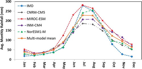
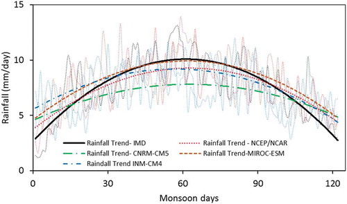
The impact of climate change on the ISMR poses a major threat to water resource management in highly populated countries, such as India. Reliable projection of future ISMR is very important to adopt changes in the water balance components. Saha et al. (2014) reported that the CMIP5 models, with few exceptions, failed to capture the decreasing trend of the ISMR post-1950. Evaluation of the CMIP5 models is recommended before their use to improve the reliability of future projections and policy adaptation. Accordingly, the available GCMs were investigated based on previous studies (Saha et al. 2014, Sharmila et al. 2015) and four GCMs (CNRM-CM5, MIROC-ESM, INM-CM4 and NorESM1-M) were selected. The rainfall trend simulated by the GCMs and the observed rainfall by the IMD were plotted for the historical period of 1950–2005. Figure 4 shows that CNRM-CM5, MIROC-ESM, INM-CM4 and NorESM1-M have a decreasing trend for ISMR post-1950. Hence, these GCMs were selected to project the future daily rainfall (2011–2100) in the GRB. Figure 5 presents the seasonal cycle of ISMR using IMD data and the selected CMIP5 model simulations, averaged for the period 1951–2005. The MIROC-ESM overestimated the monsoon rainfall, whereas the NorESM1-M produced a series nearly matching the observed IMD rainfall data, except for underestimation in June. The INM-CM4 and CNRM-CM5 models underestimated the rainfall. The deviation in capturing the rainfall magnitude by the selected CMIP5 models may be because of model uncertainties and limitations of the models in capturing geophysical processes. However, despite the deviation in magnitude, all the models reasonably captured the seasonal rainfall cycle.

Figure 4. Observed and GCM-simulated rainfall trends for ISMR averaged over the period 1951–2005: (a) observed IMD, (b) CNRM-CM5, (c) MIROC-ESM, (d) INM-CM4, and (d) NorESM1-M.

Figure 5. Seasonal cycle of monthly ISMR using IMD (observed) and four CMIP5 model simulations (historical), averaged over the period 1951–2005.

The selection of these GCMs is further strengthened by previous studies. Sharmila et al. (2015) defined the criteria to evaluate the performance of CMIP5 models in simulating the basic characteristics of the ISMR; the INM-CM4 and NorESM1-M performed better in simulating the ISMR. Shashikanth et al. (2014) evaluated the performance of different models in projecting the future rainfall for RCP4.5 at different resolutions. They reported that the CNRM-CM5 and MIROC-ESM models more accurately simulated the plausible changes in the projected rainfall. Considering these discussions and selection criteria, simulated climate variables of the four CMIP5 models were used to obtain more accurate projections of rainfall in the GRB.

5.3 Bias correction

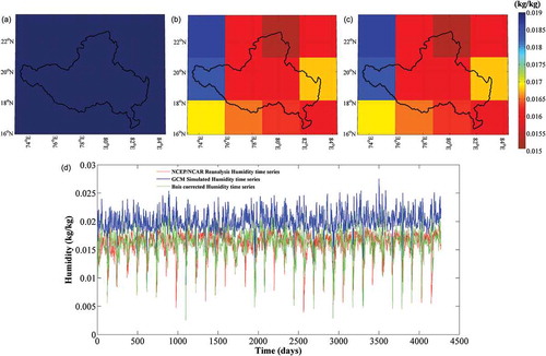
The GCM outcomes cannot be used directly in the downscaling technique because of the bias in the GCM-simulated data series. This might have been introduced because of a lack of understanding of the geophysical processes, assumptions adopted in the models and the numerical and parameterization schemes used. The removal of systematic differences between the observed and GCM-simulated climate variables is known as bias correction (Li et al. 2010). Figure 6 shows a comparison of three humidity datasets in space and time for the period 1971–2005 in the GRB. Comparison of Figure 6(a) and (b) shows that the uncorrected GCM-simulated humidity fails to capture the spatial variation as observed humidity. Figure 6(d) presents the systematic bias between these two data series at the sample grid level. This may be because of the lack of understanding of the geophysical processes, which results in assumptions being made during GCM development that reduce the accuracy of GCMs in simulating climate variables. Comparison of Figure 6(b) and (c) indicates that bias-corrected GCM-simulated humidity represents the spatial variation as observed humidity in the basin. Figure 6(d) presents the match between these two data series after eliminating the bias. Hence, correction of the systematic bias in GCM output for historical and future data series is required for the accurate projection of climate variables.

Figure 6. Bias correction applied humidity during monsoon for 1971–2005 over the Godavari River Basin: (a) uncorrected GCM simulations – spatial distribution; (b) NCEP/NCAR reanalysis data – spatial distribution; (c) bias-corrected GCM simulations – spatial distribution; and (d) comparison of different time series of specific humidity.

5.4 Principal component analysis

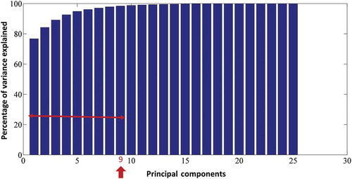
Bias-corrected data are multidimensional and highly correlated; hence, they cannot be used directly in the statistical downscaling model. The number of dimensions in data is significantly reduced using the PCA technique, without hampering the variability in the original dataset. The reduction in the number of dimensions results in a significant decrease in computation effort. Figure 7 shows a pictorial representation of the PC for surface temperature. The observed surface temperature time series obtained from NCEP/NCAR data is available at 2.5° resolution. Twenty-five predictors are available for the Godavari region; accounting for all these predictors would result in multidimensionality and multicollinearity. Hence, only nine predictors (Fig. 7), which explained the 98% variability in surface temperature, were considered for the future projection of climate variables. In the same way, PCs for other climatic variables, such as geopotential height, near-surface specific humidity, specific humidity at 500-hPa pressure level, mean sea level pressure and U-wind and V-wind at the surface level, as well as 500-hPa pressure level, were obtained. The PCs of all the climate variables collectively were considered for statistical downscaling.

Figure 7. Cumulative percentage of variance explained by NCEP/NCAR principal components (PC) for surface temperature (98% variability), shown with PC number.

5.5 Performance of the statistical downscaling model

The performance and accuracy of the downscaling model were evaluated by comparing the projected spatial variations of the simulated rainfall derived using NCEP/NCAR reanalysis data and the observed rainfall. Figure 8 compares the statistical mean of the daily observed and daily projected rainfall in the GRB for the testing period (1991–2005). The agreement between Figure 8(a) and (b) shows that the spatial variation of the observed mean rainfall is very well depicted by the projected rainfall (by using NCEP/NCAR reanalysis data predictors). The average projected rainfall of 919.78 mm is slightly less than the average observed rainfall (930.47 mm). The absolute difference, ranging from −2 to +2 mm for most grids (more than 90% of the grids), indicates good agreement between the observed and projected rainfall (see Supplementary material, Fig. S1). Comparison of Figure 9(a) and (b) shows that the projected rainfall well replicates the spatial distribution of the standard deviation (SD) of the observed rainfall. The absolute difference in the SD (range: −6 to 6 mm/d) for most grids (>80% grids), indicates good agreement between the observed and projected rainfall (see also Fig. S1). Furthermore, the rainfall was projected for RCP4.5 and RCP8.5 scenarios using simulated predictors for the selected GCMs. The projected rainfall was then compared with the observed rainfall to evaluate the performance of the GCMs in projecting the rainfall for the historical period at the river-basin scale. Figures 8(c)–(f) and 9(c)–(f) show that the spatial pattern of the mean and standard deviation was replicated reasonably well by the four GCMs. The MIROC-ESM projects the highest rainfall, whereas CNRM-CM5 projects the lowest rainfall, which is in agreement with the historical simulations (1951–2005) of rainfall by these GCMs (Fig. 5). Figure 10 presents cross-correlation plots between the observed and model-projected rainfall for the testing period for the entire grid in the GRB. Figure 10 illustrates that the cross-correlation among the gridded observed rainfall data is well replicated by the projected rainfall data using NCEP/NCAR reanalysis data and climate variables simulated by the four GCMs. Figure 11 shows the seasonal cycle depicted by the projected rainfall using climate variables simulated by the four GCMs for the testing period. The trend presented by all the models is the same as that presented by the observed rainfall. Rainfall projections obtained by adopting the NCEP/NCAR and GCM predictors mainly validate the model proposed by Kannan and Ghosh (2013), as well as evaluating the performance of the GCMs.

Figure 8. Comparison of means of observed and projected downscaled GCM-simulated monsoon rainfall (CMIP5) for the Godavari River Basin at 0.25° resolution for 1991–2005: (a) IMD (observed rainfall), (b) NCEP/NCAR (projected rainfall), (c) CNRM-CM5, (d) MIROC-ESM, (e) INM-CM4, and (f) NorESM1-M.

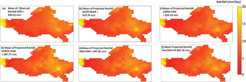
Figure 9. Comparison of standard deviation of observed and projected downscaled GCM-simulated rainfall (CMIP5) for the Godavari River Basin at 0.25° resolution for 1991–2005: (a) IMD (observed rainfall), (b) NCEP/NCAR (projected rainfall), (c) CNRM-CM5, (d) MIROC-ESM, (e) INM-CM4, and (f) NorESM1-M.

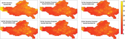
Figure 10. Scatterplots for cross-correlation of multisite rainfall between observed and GCM projected: (a) IMD and NCEP/NCAR, (b) IMD and CNRM-CM5, (c) IMD and MIROC-ESM, (d) IMD and INM-CM4, and (d) IMD and NorESM1-M.

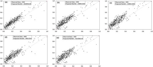
Figure 11. Seasonal cycle of daily ISMR using IMD (observed) and four CMIP5 model projections (historical), averaged over the testing period (1991–2005).

5.6 Future projections of ISMR

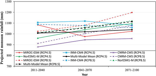
The rainfall for the near future (2011–2040), mid future (2041–2070) and far future (2071–2100) periods under RCP4.5 and RCP8.5 scenarios was projected using climate variables for the four GCMs (Fig. 12). An increasing trend was observed for NorESM1-M and CMRM-CM5, whereas trends were inconsistent for MIROC-ESM and INM-CM4 under the RCP4.5 and RCP8.5 scenarios. For MIROC-ESM, the trend decreases from near future (2011–2040) to mid future (2041–2070) and increases from mid future (2041–2070) to far future (2071–2100) under RCP4.5, whereas it increases under RCP8.5. For INM-CM4, the trend of the projected future rainfall is exactly the reverse of that by MIROC-ESM under RCP4.5, and it decreases under RCP8.5. The trends in the ISMR projections obtained using climate variables simulated by INM-CM4 and MIROC-ESM models are inconsistent with respect to the time and scenarios.

Figure 12. Future projected rainfall using GCM-simulated climate variables and multi-model mean rainfall under the RCP4.5 and RCP8.5 scenarios over the Godavari River Basin for different time slices.

For the projected future rainfall obtained using climate variables simulated by different GCMs for different time slices under RCP4.5 and RCP8.5, refer to the Supplementary material (Figs S2 and S3, respectively). Figures 13(a), (d), (h) and 14(a), (d), (h) provide the spatial pattern of changes in the projected rainfall relative to the present climate, using the multi-model mean for different time slices in the GRB, under RCP4.5 and RCP8.5, respectively. These plots show that the spatial pattern of the projected rainfall and relative changes are not modified significantly in the GRB under either scenario. To further explore the climate change within the river basin, projected hydrological variables were obtained at Tekra station (Fig. 1; catchment area: 10 8780 km²). Table 4(a) presents the multi-model mean of the projected hydrological variables derived using the VIC model for the present climate for GRB and the Tekra catchment, and Table 4(b) presents the multi-model mean of the projected hydrological variables for three time slices under the RCP4.5 and RCP8.5 scenarios in the GRB. Table 5(a) presents the increase in the projected multi-model mean rainfall for three time slices relative to the present climate in the GRB. Rainfall increases are in the ranges 9.89–13.38% and 10.06–21.53% under RCP4.5 and RCP8.5, respectively. Future changes are also found to be more robust under RCP8.5 than under RCP4.5, which is in agreement with a previous study (Kitoh et al. 2013). Tables 4(c) and 5(b) present the increase in the projected multi-model mean rainfall and percentage change for the Tekra catchment, respectively. The increasing rainfall trend for the Tekra catchment is consistent with that in the GRB, although there is a small change in magnitude.

Table 4. Multi-model mean for present and future projected hydrological variables for the RCP4.5 and RCP8.5 scenarios over the Godavari River Basin (GRB).

(a) Present hydrological variables
Catchment	Period	Rainfall (mm)	Surface runoff (mm)		Baseflow (mm)		Evapotranspiration (mm)
GRB	1991–2005	916.49	169.64		91.82		512.36
Tekra	1991–2005	921.75	170.4		92.68		524.97
(b) GRB: projected hydrological variables
	Rainfall (mm)		Surface runoff (mm)		Baseflow (mm)		Evapotranspiration (mm)
Period	RCP4.5	RCP8.5	RCP4.5	RCP8.5	RCP4.5	RCP8.5	RCP4.5	RCP8.5
2011–2040	1007.16	1008.68	178.80	173.46	144.84	139.39	536.41	544.08
2041–2070	1019.70	1055.14	178.59	188.70	146.05	159.95	551.66	555.27
2071–2100	1039.12	1113.79	187.82	214.53	154.84	177.98	550.88	567.02
(c) Tekra catchment: projected hydrological variables
	Rainfall (mm)		Surface runoff (mm)		Baseflow (mm)		Evapotranspiration (mm)
Period	RCP4.5	RCP8.5	RCP4.5	RCP8.5	RCP4.5	RCP8.5	RCP4.5	RCP8.5
2011–2040	988.36	994.43	172.96	176.85	120.22	115.16	549.13	563.20
2041–2070	1033.50	1089.83	174.76	194.73	130.93	158.09	566.47	575.94
2071–2100	1066.67	1226.22	191.59	244.64	152.22	210.70	562.66	594.65

Table 5. Changes in multi-model means between present and projected hydrological variables for the RCP4.5 and RCP8.5 scenarios.

A) Godavari River Basin
	Rainfall (%)		Surface Runoff (%)		Baseflow (%)		Evapotranspiration (%)
Time	RCP4.5	RCP8.5	RCP4.5	RCP8.5	RCP4.5	RCP8.5	RCP4.5	RCP8.5
2011-2040	9.89	10.06	5.40	2.25	71.96	51.81	4.69	6.19
2041-2070	11.26	15.13	5.28	11.24	74.15	74.20	7.67	8.38
2071-2100	13.38	21.53	10.72	26.47	84.43	93.84	7.52	10.67
B) Tekra catchment
	Rainfall (%)		Surface Runoff (%)		Baseflow (%)		Evapotranspiration (%)
Time	RCP4.5	RCP8.5	RCP4.5	RCP8.5	RCP4.5	RCP8.5	RCP4.5	RCP8.5
2011-2040	7.23	7.89	1.50	3.79	29.72	24.26	4.60	7.28
2041-2070	12.12	18.23	2.56	14.28	41.27	70.58	7.91	9.71
2071-2100	15.72	33.03	12.44	43.57	64.24	127.34	7.18	13.27

Figure 13. Spatial pattern of changes in future projected hydrological components relative to present climate under the RCP4.5 scenario using multi-model means for different time slices over the Godavari River Basin.

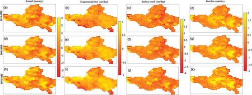
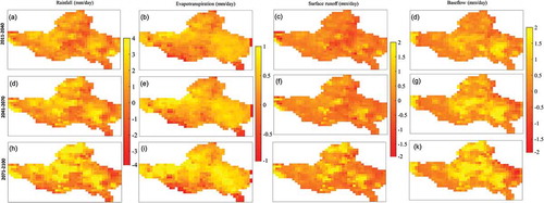
Figure 14. Spatial pattern of changes in future projected hydrological components relative to present climate under the RCP8.5 scenario using multi-model means for different time slices over the Godavari River Basin.

Table 6 presents the multi-model mean for bias-corrected and GCM-simulated future surface temperature for the baseline and future periods under the RCP4.5 and RCP8.5 scenarios. Table 6 shows an increase in future surface temperature of 0.57° (2011–2040) to 1.8° (2071–2100) under RCP4.5, and 0.67° (2011–2040) to 2.84° (2071–2100) under RCP8.5, compared to the baseline period (1971–2005). The GCM-simulated and bias-corrected future projected surface temperature for each selected GCM for different time slices under RCP4.5 and RCP8.5 are also shown in the Supplementary material (Table S3).

Table 6. Multi-model means of GCM-simulated and bias-corrected surface temperature under the RCP4.5 and RCP8.5 scenarios over the Godavari River Basin.

Period	Time slice	Surface temp. (°C)		Increase in surface temp. (°C)
Historical	1971–2005*	26.55	26.55	-	-
	Scenario	RCP4.5	RCP8.5	RCP4.5	RCP8.5
Future	2011–2040	27.12	27.22	0.57	0.67
	2041–2070	27.83	28.32	1.28	1.77
	2071–2100	28.35	29.39	1.80	2.84

* Baseline.

5.7 Projections of hydrological variables: VIC model

The impacts of climate change on the hydrology of the GRB were investigated by assessing the changes in the water balance components for three future time slices (2011–2040, 2041–2070 and 2071–2100) under the RCP4.5 and RCP8.5 scenarios relative to the present climate. The VIC model-derived multi-model means of hydrological variables simulated using the projected rainfall for the testing period were considered as hydrological variables for the present climate (shown in Fig. S4). The projected rainfall, the GCM-simulated and bias-corrected wind speed, as well as minimum and maximum daily temperature, were used as input to run the VIC model. The VIC model runs were explicitly conducted for each time slice and GCM. The multi-model means of the VIC-simulated hydrological variables in the GRB were simulated for each time slice under RCP4.5 (shown in Fig. S5) and RCP8.5 (shown in Fig. S6). The spatial pattern of changes in the future projected hydrological components relative to the present climate obtained using the multi-model means for different time slices in the GRB is presented in Figure 13 (RCP4.5) and Figure 14 (RCP8.5). The future projected hydrological variables obtained using the future rainfall projected from GCMs and the VIC model were simulated under RCP4.5 and RCP8.5 (the absolute values are presented in Tables S1 and S2, respectively). Table 4(b) presents the absolute multi-model mean for the projected hydrological variables, and Table 5(a) presents the changes (%) in the multi-model mean for the projected hydrological variables relative to the present climate for the future in the GRB under both scenarios.

Figure 13 shows that the spatial pattern of changes in rainfall indicates an increase in the rainfall by 1–4 mm/d for most grid cells. A few grid cells show an insignificant decrease in rainfall of up to −2 mm/d. From the results presented in Table 5(a), an increase in rainfall is observed in the GRB in both time and space. The spatial pattern of evapotranspiration shows a nominal increase of up to 1 mm/d for all the time slices (Fig. 13) and total change relative to the present climate ranges from 4.69% (2011–2040) to 7.67% (2041–2070). A decrease in evapotranspiration is observed at only a few grids. An increase of up to 2 mm/d is observed in the simulated surface runoff for most grids, while a decrease of up to 1 mm/d is observed for some grids (Fig. 13). The increase in surface runoff ranges from 5.4 to 10.72% for the future time periods. The baseflow increased at the highest rate (range: 71.96–84.43%) compared to evapotranspiration and surface runoff. The hydrological changes under RCP8.5 are higher than those under RCP4.5, which is expected because of the increased future projected rainfall under RCP8.5. Furthermore, the proportionate increase in the hydrological variables (Table 5(a)) shows that the hydrological model can reasonably translate the impact of climate change at the river-basin scale. Tables 4(c) and 5(b) present an increase in the projected multi-model mean for hydrological variables and percentage change, respectively, for the Tekra catchment. The increasing trend in hydrological variables for the Tekra catchment is consistent with that of the GRB and is in proportion with rainfall increase.

5.8 Discussion

In this study, the VIC-2L model was used to assess climate change impacts on the hydrology of the GRB in peninsular India. The model calibration and validation showed reasonable agreement between observed and simulated flows at Polavaram station, demonstrating the suitability of the VIC model to simulate the GRB hydrology. Using the performance rating of N_s and PBIAS (Moriasi et al. 2007), the N_s value (>0.75) of this study indicated very good performance of the model, whereas PBIAS (<20%) indicated that the VIC model performance was satisfactory. Thompson et al. (2013) reported substantial uncertainty in projected river flows, and emphasized that the uncertainty in the hydrological model should not be overlooked. Further, the results of the VIC hydrological model have been reported by Hengade and Eldho (2016) for Ashti catchment (area: 50 990km²), a sub-basin of the GRB, and the GRB up to its outlet at Polavaram station (catchment area: 307 800km²). Their results showed the model performance at a different spatial scale, and indicated that the simulated streamflows were in good agreement with observed streamflow. They showed the effectiveness of the VIC model to evaluate hydrological changes from a medium-sized catchment to a large-scale river basin satisfactorily.

The kernel regression-based downscaling technique alone generally fails to model multi-site rainfall between stations. Kannan and Ghosh (2013) and Salvi et al. (2013) reported that the kernel regression-based downscaling approach combined with the CART model performed better in simulating multisite ISMR. The kernel regression-based downscaling technique captured the mean and spatial pattern of standard deviation reasonably well, but failed to model the climatology (Salvi et al. 2013). To overcome this limitation, we adopted the modified methodology proposed by Salvi et al. (2013) in this study. The bias correction for each month was carried out separately for the monsoon period (JJAS), and PCA was applied on each individual climate variable. The results of future daily rainfall projections show that all GCMs perform reasonably well in capturing the spatial pattern and consistent variations in rainfall magnitudes for projections and historical simulations.

The inconsistent trend of the future projected rainfall represented by MIROC-ESM and INM-CM4 (Fig. 12) may be due to the lack of capability of the CMIP5 models in capturing large-scale changes (Saha et al. 2014). Secondly, it may be due to the uncertainty in the physical and mathematical formulations of the geophysical processes, different initial conditions, parameterization and assumptions. Furthermore, the CMIP5 models failed to simulate the cyclonic formation in the Pacific region, probably accounting for the inconsistent ISMR projections (Saha et al. 2014). The improved representation of geophysical processes may increase the reliability of the ISMR projections. Furthermore, the strength of the model is indicated by the plots of cross-correlation among the gridded observed rainfall data and projected rainfall data obtained by using NCEP/NCAR reanalysis data and climate variables simulated by the four GCMs.

Das and Umamahesh (2016) projected an increasing rainfall trend for the RCP2.6 and RCP 4.5 scenarios and a mixed rainfall trend (mostly increasing trend) for the RCP8.5 scenario over the GRB using single a GCM, the Canadian Earth System Model (CanESM2). Our study showed an increase in projected future rainfall (multi-model mean) under RCP4.5 and RCP8.5 scenarios in the GRB for the entire 21st century, with a higher increase for the RCP8.5 scenario. Ramesh and Goswami (2014) suggested the use of better models for regional climate projections. The multi-model mean shows an increase in the ISMR in the study area. Kitoh et al. (2013) and Lee and Wang (2012) indicated a significant increase in the global monsoon rainfall. Goswami (2011) projected an increase in the global monsoon intensity and amount. Meenu et al. (2013) reported that climate change increased the ISMR in the catchment area of the Tunga-bhadra River. Hence, the projected increase in the ISMR in the GRB is in agreement with the aforementioned studies.

As observed, the increase in rainfall increases the other dependent water balance components. Notably, the rate of increase in evapotranspiration is the lowest (4.69–7.52% and 6.19–10.67% for RCP4.5 and RCP8.5, respectively) amongst all hydrological variables (Table 5). Firstly, this may be because the soil is fully saturated during the monsoon season and any change in rainfall does not contribute further to the evapotranspiration. Eventually, change in rainfall contributes predominantly to surface runoff and baseflow. Secondly, the potential evapotranspiration is governed predominantly by the land-cover class. Typically, evapotranspiration is higher in forest areas than in nonforest areas, as the deeper roots draw more water from the soil (Zhang et al. 2001). Our study was restricted to accessing the hydrological changes caused by changes in the future projected rainfall because constant land cover obtained from AVHRR was employed for all the time slices. The constant land cover may be one of the reasons for the small change in evapotranspiration rate in the future time slices. The higher rate of increase in baseflow may be because the thicker bottom soil layer causes a higher retention of soil moisture, which eventually contributes to higher baseflow. Hence, it can be concluded that the increased rainfall contributes predominantly to the total runoff (surface runoff plus baseflow), whereas its contribution to evapotranspiration is limited. The projected trend and change in hydrological variables for future time slices for the Tekra catchment (108 780 km²) are consistent with the trend and change in hydrological variables over the entire GRB. This implies that the impact of climate changes within the GRB are consistent.

6 Conclusions

This study evaluated the implications of climate change for the hydrology of a large river basin in India, the Godavari River Basin (GRB), using projected Indian summer monsoon rainfall (ISMR) for a future period (2011–2100). The ISMR projections were obtained using climate variables for selected global climate models (GCMs) and a kernel regression-based statistical downscaling model. The hydrology of the basin was modelled using the VIC macroscale hydrological model. The major conclusions of the study are as follows:

• The VIC model accounts for a large number of data, such as topography, land cover, soil, precipitation and wind speed, and minimum and maximum temperature, to represent the physical, meteorological and hydrological characteristics of the river basin. The assessment of climate change using the VIC model is further strengthened by the readily available global or regional gridded dataset. The agreement between the observed and simulated streamflow is evaluated using performance criteria (the N_s value, PBIAS and R²). The results for the calibration and validation periods showed the capability of the VIC model to simulate the river basin hydrology. The over-prediction or under-prediction of extreme flows is an inherent problem in hydrological modelling of a basin due to the lack of modelling capability to simulate extreme events.

• Judicious selection criteria were used to select the most realistic CMIP5 climate models for simulating ISMR trend and variability, because most of these models fail to simulate the post-1950 decreasing trend of the ISMR. Four GCMs – CNRM-CM5, MIROC-ESM, INM-CM4 and NorESM1-M – were selected for further climate change simulations. Rainfall projection results for the testing period showed that all the models consistently simulated the ISMR and matched the observed rainfall.

• The GCM-simulated climate variables from a coarser resolution were downscaled to derive finer resolution inputs required by the hydrological model by using a kernel regression-based downscaling technique. The statistical downscaling model performed well in capturing the mean, standard deviation, spatial pattern and seasonal variability of rainfall during the testing period.

• The multi-model mean ISMR projection showed an increasing trend in the GRB. The spatial pattern of future rainfall projections is identical to that of the observed historical rainfall.

• The increase in rainfall increases the other dependent water balance components, namely surface runoff, baseflow and evapotranspiration. However, the rate of increase in evapotranspiration was low (4.69–7.52% and 6.19–10.67% for RCP4.5 and RCP8.5, respectively) compared with that for surface runoff and baseflow. This indicates that evapotranspiration is governed predominantly by the land-cover class, which is constant in the present study for all future slices, whereas higher changes in runoff processes showed that these processes are dominated by rainfall. Furthermore, the results reveal that the VIC hydrological model effectively translates the effect of climate changes on the hydrological variables.

• The smaller changes in the basin hydrology showed the GRB as a stable basin considering the hydrological implications of climate change. This provides an opportunity for the effective planning and adaptation of stable long-term water resource policies in the river basin by considering the present climate as the baseline and dynamic policies for the variations in hydrology for the future.

• The outcome of the study may be used to define water resource management policies within the GRB. Further, the methodology can be adopted to assess climate change impacts on larger river basins worldwide.

Acknowledgements

The authors sincerely acknowledge the Central Water Commission (CWC) for providing streamflow data at various locations in the GRB. The authors express their sincere gratitude to the editor and reviewers for their critical comments which helped to improve the manuscript significantly. The third author thanks the Ministry of Earth Sciences for partial support.

Disclosure statement

No potential conflict of interest was reported by the authors.

Supplemental data

Supplementary material can be accessed here.

References

- Baldassarre, D., et al., 2011. Future hydrology and climate in the River Nile basin: a review. Hydrological Sciences Journal, 56 (2), 199–211. doi:10.1080/02626667.2011.557378
- Chiew, F. and McMahon, T., 1993. Detection of trend or change in annual flow of Australian rivers. International Journal of Climatology, 13, 643–653. doi:10.1002/(ISSN)1097-0088
- Cuo, L., et al., 2013. The impacts of climate change and land cover/use transition on the hydrology in the upper Yellow River Basin, China. Journal of Hydrology, 502, 37–52. doi:10.1016/j.jhydrol.2013.08.003
- Das, J. and Umamahesh, N.V., 2016. Downscaling monsoon rainfall over river Godavari Basin under different climate change scenarios. Water Resources Management, 30, 5575–5587. doi:10.1007/s11269-016-1549-6
- Deshpande, N.R., Kothawale, D.R., and Kulkarni, A., 2016. Changes in climate extremes over major river basins of India. International Journal of Climatology, 36, 4548–4559. doi:10.1002/joc.2016.36.issue-14
- Dibike, Y. and Coulibaly, P., 2007. Validation of hydrological models for climate scenario simulation: the case of Saguenay Watershed in Quebec. Hydrological Processes, 2123, 3123–3135. doi:10.1002/hyp.6534
- Dionysia, P., 1992. Impacts of GISS-modelled climate changes on catchment hydrology. Hydrological Sciences Journal, 37 (2), 141–163. doi:10.1080/02626669209492574
- Dobler, A. and Ahrens, B., 2011. Four climate change scenarios for the Indian summer monsoon by the regional climate model COSMO-CLM. Journal of Geophysical Research, 116, 1–13. doi:10.1029/2011JD016329
- Dunn, S., 1998. Large scale modelling using small scale processes. In: H. Wheater and C. Kirby, eds. Hydrology in a changing environment. Chichester, UK: Wiley, 11–20.
- FAO, 2003. The digitized soil map of the world and derived soil properties version 3.5. FAO Land and Water Digital Media Series 1. Rome: FAO.
- Fowler, H., Blenkinsop, S., and Tebaldi, C., 2007. Linking climate change modelling to impacts studies: recent advances in downscaling techniques for hydrological modelling. International Journal of Climatology, 27, 1547–1578. doi:10.1002/(ISSN)1097-0088
- Gadgil, S. and Rupa Kumar, K., 2006. The Asian monsoon-agriculture and economy. In: B. Wang, ed. The Asian monsoon. Berlin, Germany: Springer, 651–683.
- Gao, H., et al., 2010. Water budget record from variable infiltration capacity VIC model. In: E.F. Wood, ed. Algorithm theoretical basis document for terrestrial water cycle data records. in review.
- Githui, F., et al., 2009. Climate change impact on SWAT simulated streamflow in western Kenya. International Journal of Climatology, 29, 1823–1834. doi:10.1002/joc.v29:12
- Goswami, B., 2011. South Asian summer monsoon. In: W.K.-M. Lau and D.E. Waliser, eds. Intraseasonal variability of the atmosphere–ocean climate system. 2nd ed. Berlin, Germany: Springer, 21–72.
- Hamlet, A. and Lettenmaier, D., 1999. Effects of climate change on hydrology and water resources in the Columbia River basin. Journal of American Water Resources Association, 356, 1597–1623. doi:10.1111/j.1752-1688.1999.tb04240.x
- Hay, L., Markstrom, S., and Ward-Garrison, C., 2011. Watershed-scale response to climate change through the twenty-first century for selected basins across the United States. Earth Interactions, 15, 1–37. doi:10.1175/2010EI370.1
- Hengade, N. and Eldho, T., 2016. Assessment of LULC and climate change on the hydrology of Ashti Catchment, India using VIC model. Journal of Earth System Science, 1258, 1623–1634. doi:10.1007/s12040-016-0753-3
- Hewitson, B. and Crane, R., 1996. Climate downscaling: techniques and application. Climate Research, 7, 85–95. doi:10.3354/cr007085
- Jaewon, J., et al., 2017. Hydrological responses to climate shifts for a minimally disturbed mountainous watershed in Northwest China. Hydrological Sciences Journal. doi:10.1080/02626667.2017.1316851
- Kalnay, E., Kanamitsu, M., and Kistler, R., 1996. The NCEP/NCAR 40- years reanalysis project. Bulletin of the American Meteorological Society., 773, 437–471. doi:10.1175/1520-0477(1996)077<0437:TNYRP>2.0.CO;2
- Kannan, S. and Ghosh, S., 2013. A nonparametric Kernel regression model for downscaling multisite daily precipitation in the Mahanadi basin. Water Resources Research, 49, 1360–1385. doi:10.1002/wrcr.20118
- Kishtawal, C., et al., 2009. Urbanization signature in the observed heavy rainfall. Climatology over India. International Journal of Climatology, 30, 1908–1916. doi:10.1002/joc.2044
- Kitoh, A., et al., 2013. Monsoons in a changing world: A regional perspective in a global context. Journal of Geophysical Research - Atmospheres, 118, 3053–3065. doi:10.1002/jgrd.50258
- Kling, H. and Gupta, H., 2009. On the development of regionalization relationships for lumped watershed models: the impact of ignoring sub-basin scale variability. Journal of Hydrology, 373, 337–351. doi:10.1016/j.jhydrol.2009.04.031
- Lee, J.-Y. and Wang, B., 2012. Future change of global monsoons in the CMIP5. Climate Dynamics, 42, 101–119. doi:10.1007/s00382-012-1564-0
- Li, H., Sheffield, J., and Eric, F., 2010. Bias correction of monthly precipitation and temperature fields from Intergovernmental Panel on Climate Change AR4 models using equidistant quantile matching. Journal of Geophysical Research - Atmospheres, 115, 1–20.
- Liang, X., et al., 1994. A simple hydrologically based model of land surface water and energy fluxes for general circulation models. Journal of Geophysical Research - Atmospheres, 99, 14415–14428. doi:10.1029/94JD00483
- Lohmann, D., et al., 1998. Regional scale hydrology: I. Formulation of the VIC-2L model coupled to a routing model. Hydrological Sciences Journal, 43, 31–141.
- Mao, D. and Cherkauer, K., 2009. Impacts of land-use change on hydrologic responses in the Great Lakes region. Journal of Hydrology, 3741 (2), 71–82. doi:10.1016/j.jhydrol.2009.06.016
- Maraun, D., et al., 2010. Precipitation downscaling under climate change: recent developments to bridge the gap between dynamical models and the end user. Reviews of Geophysics, 48, 1–34. doi:10.1029/2009RG000314
- Maurer, E., et al., 2002. A long-term hydrologically-based data set of land surface fluxes and states for the conterminous United States. Journal of Climate, 15, 3237–3251. doi:10.1175/1520-0442(2002)015<3237:ALTHBD>2.0.CO;2
- Meenu, R., Rehana, S., and Mujumdar, P., 2013. Assessment of hydrologic impacts of climate change in Tunga-Bhadra river basin, India with HEC-HMS and SDSM. Hydrological Processes, 27, 1572–1589. doi:10.1002/hyp.v27.11
- Menon, A., Levermann, A., and Schewe, J., 2013. Enhanced future variability during India’s rainy season. Geophysical Research Letters, 40, 3242–3247. doi:10.1002/grl.50583
- Moriasi, D., et al., 2007. Model evaluation guidelines for systematic quantification of accuracy in watershed simulations. American Society of Agricultural and Biological Engineers, 50 (3), 885−900.
- Nijssen, B., et al., 2001. Hydrologic sensitivity of global rivers to climate change. Climatic Change, 50, 143–175. doi:10.1023/A:1010616428763
- Nijssen, B., O’Donnell, G., and Lettenmair, D., 2000. Predicting the discharge of global rivers. Journal of Climate, 14, 3307–3323. doi:10.1175/1520-0442(2001)014<3307:PTDOGR>2.0.CO;2
- Pai, D.S., et al., 2014. Development of a new high spatial resolution (0.25° X 0.25°) Long period (1901-2010) daily gridded rainfall dataset over India and its comparison with existing datasets over the region. Mausam, 65-1, 1–18.
- Ramesh, K. and Goswami, P., 2014. Assessing reliability of regional climate projections: the case of Indian monsoon. Scientific Reports, 4-4071, 1–9.
- Rehana, S. and Mujumdar, P., 2011. River water quality response under hypothetical climate change scenarios in Tunga–bhadra river, India. Hydrological Processes, 25, 3373–3386. doi:10.1002/hyp.8057
- Riahi, K., et al., 2011. RCP 8.5—A scenario of comparatively high greenhouse gas emissions. Climatic Change, 109, 33–57. doi:10.1007/s10584-011-0149-y
- Saha, A., et al., 2014. Failure of CMIP5 climate models in simulating post-1950 decreasing trend of Indian monsoon. Geophysical Research Letters, 41, 7323–7330. doi:10.1002/2014GL061573
- Salvi, K., Ghosh, S., and Kannan, S., 2013. High-resolution multisite daily rainfall projections in India with statistical downscaling for climate change impacts assessment. Journal of Geophysical Research - Atmospheres, 118, 3557–3578. doi:10.1002/jgrd.50280
- Schoof, J., 2013. Statistical downscaling in climatology. Geographical Compass, 74, 249–265. doi:10.1111/gec3.12036
- Shah, H. and Mishra, V., 2016. Hydrologic changes in Indian subcontinental river basins (1901–2012). American Meteorological Society, 2667–2687. doi:10.1175/JHM-D-15-0231.1
- Sharmila, S., et al., 2015. Future projection of Indian summer monsoon variability under climate change scenario: an assessment from CMIP5 climate models. Global and Planetary Change, 124, 62–78. doi:10.1016/j.gloplacha.2014.11.004
- Shashikanth, K., et al., 2013. Do CMIP5 simulations of Indian summer monsoon rainfall differ from those of CMIP3? Atmospheric Science Letters, 15, 79–85. doi:10.1002/asl2.466
- Shashikanth, K., et al., 2014. Comparing statistically downscaled simulations of Indian monsoon at different spatial resolutions. Journal of Hydrology, 519, 3163–3177. doi:10.1016/j.jhydrol.2014.10.042
- Shepard, D. (1968). A two-dimensional interpolation function for irregularly spaced data. In: Proceedings of the 1968 23rd ACM national conference, (ACM ’68), ACM, New York, NY, USA, 517–524. doi:10.1145/800186.810616.
- Srivastava, A.K., Rajeevan, M., and Kshirsagar, S.R., 2009. Development of a high resolution daily gridded temperature dataset (1969–2005) for the Indian region. Atmospheric Science Letters, 10, 249–254.
- Thompson, J.R., Crawley, A., and Kingston, D.G., 2016. GCM-related uncertainty for river flows and inundation under climate change: the Inner Niger Delta. Hydrological Sciences Journal, 61, 2325–2347. doi:10.1080/02626667.2015.1117173
- Thompson, J.R., et al., 2013. Assessment of uncertainty in river flow projections for the Mekong River using multiple GCMs and hydrological models. Journal of Hydrology, 486, 1–30. doi:10.1016/j.jhydrol.2013.01.029
- Thomson, A.M., et al., 2011. RCP4.5: a pathway for stabilization of radiative forcing by 2100. Climatic Change. doi:10.1007/s10584-011-0151-4
- Todini, E., 1996. The ARNO rainfall-runoff model. Journal of Hydrology, 175, 339–382. doi:10.1016/S0022-1694(96)80016-3
- Webster, P., et al., 1998. Monsoons: processes, predictability and the prospects for prediction. Journal of Geophysical Research, 103, 14451–14510. doi:10.1029/97JC02719
- Wilby, R., Charles, S., and Zorita, E. (2004). The guidelines for use of climate scenarios developed from statistical downscaling methods. Supporting material of the Intergovernmental Panel on Climate Change IPCC, prepared on behalf of Task Group on Data and Scenario Support for Impacts and Climate Analysis TGICA. Available from: http://ipccddc.cru.uea.ac.uk/guidelines/StatDownGuide.pdf.
- Xu, C., 1999. Climate change and hydrologic models: a review of existing gaps and recent research developments. Water Resources Management, 135, 369–382. doi:10.1023/A:1008190900459
- Xu, J., et al., 2011. The Nonlinear trend of runoff and its response to climate change in the Aksu River western China. International Journal of Climatology, 31, 687–695. doi:10.1002/joc.v31.5
- Yu, P. and Wang, Y., 2009. Impact of climate change on hydrological processes over a basin scale in Northern Taiwan. Hydrological Processes, 23, 3556–3568. doi:10.1002/hyp.v23:25
- Zhang, L., Dawes, W., and Walker, G.R., 2001. Response of mean annual evapotranspiration to vegetation changes at catchment scale. Water Resources Research, 373, 701–708. doi:10.1029/2000WR900325
- Zhao, R., et al., 1980. The Xinanjiang model. Hydrological forecasting. Proceedings Oxford Symposium, 129, 351–356.