Estimation of the added value of using rainfall–runoff transformation and statistical models for seasonal streamflow forecasting

ABSTRACT

Two methods for generating streamflow forecasts in a Sahelian watershed, the Sirba basin, were compared. The direct method used a linear relationship to relate sea-surface temperature to annual streamflow, and then disaggregated on a monthly time scale. The indirect method used a linear relationship to generate annual precipitation forecasts, a temporal disaggregation to generate daily precipitation and the SWAT (Soil and Water Assessment Tool) model to generate monthly streamflow. The accuracy of the forecasts was assessed using the coefficient of determination, the Nash-Sutcliffe coefficient and the Hit score, and their economic value was evaluated using the cost/loss ratio method. The results revealed that the indirect method was slightly more effective than the direct method. However, the direct method achieved higher economic value in the majority of cost/loss situations, allowed for predictions with longer lead times and required less information.

KEYWORDS:

• seasonal streamflow forecasting
• principal component analysis
• multiple linear regression
• SWAT
• statistical model
• cost/loss ratio

Editor R. Woods Associate editor C. Perrin

1 Introduction

The Sahel region in West Africa is known for its high climatic variability, which has led to successive floods and droughts in the past (Brooks 2004, Lu and Delworth 2005, Samimi et al. 2012, Sittichok et al. 2016). Precipitation variability has been identified as the main factor causing vulnerability to drought, flood events and food insecurity in the region (Kandji et al. 2006). Unexpected droughts and floods make water management and economic activities that rely on water extremely complicated; particularly agriculture, which the majority of the population depends on for food and income (Day et al. 1992). Therefore, improving the ability to predict streamflow months in advance would be extremely helpful for many involved parties in the region, including protection authorities, dam operators, industry management, individual irrigation facilities and government agencies in charge of industrial and domestic water supply.

Seasonal streamflow forecasting methods fall into two main groups: direct and indirect. The direct and indirect methods are illustrated in Figure 1. With direct methods streamflow is forecast directly, using empirical relationships between the streamflow at date t + H, and selected predictors observed prior to the date, where t is the forecast issue date and H is the lag time. Examples of variables used as predictors for streamflow forecasting include daily rainfall (Tuteja et al. 2011, Robertson et al. 2013), evapotranspiration (Yossef et al. 2013), temperature (Abudu et al. 2010) and large-scale ocean and climate indices such as El Niño Southern Oscillation (ENSO) and sea-surface temperature (SST) (Piechota et al. 1998, Karamouz and Zahraie 2004, Ionita et al. 2008, Ionita et al. 2014).

Figure 1. Classification of streamflow forecasting using direct and indirect methods.

Within the indirect methods, precipitation and possibly other climate variables are forecast first, then translated into streamflow using rainfall–runoff transformation. Precipitation forecasts can be generated using statistical models (Barnston et al. 1996, Washington and Downing 1999, Garric et al. 2002) or climate models (Rowell et al. 1992, Thiaw and Mo 2005). Variables used to forecast rainfall include SST (Folland et al. 1991, Barnston et al. 1996, Garric et al. 2002, Schepen et al. 2012), wind data (Ndiaye et al. 2011) and rainfall amounts prior to the forecast date (Abedokun et al. 1979, Nnaji 2001). When climate models are used to generate rainfall predictions, biases usually have to be corrected using Model Output Statistics (MOS) approaches (Gneiting and Raftery 2005, Bouali et al. 2008, Ndiaye et al. 2009, Gobena and Gan 2010).

Rainfall–runoff models are then used to convert forecast precipitation into streamflow for seasonal forecasting (Garbrecht et al. 2007, Tuteja et al. 2011, Wang et al 2011a, Yossef et al. 2013). The advantage of rainfall–runoff models is they provide more realistic streamflow simulations, since the physical interactions between land, climate and river characteristics in the watershed are considered. Rainfall–runoff models forced with accurate rainfall forecasts, and properly initialized using antecedent hydrological variables before the forecasts are issued, can produce reliable streamflow forecasts (Wang et al. 2011b, Yossef et al. 2013). In addition, rainfall–runoff models are less sensitive to outliers in the input data compared to statistical models. However, the rainfall–runoff model introduces additional uncertainties in the model chain. The set-up of a rainfall–runoff model requires a sound/substantial database of hydro-meteorological measurements, geological information and high computational effort.

One main approach widely used for forecasting is a statistical model. Statistical models rely on empirical relationships between historical streamflow/precipitation (predictand) and hydrological or climate variables (predictors). The predictors are not necessarily from the same region as the predictand, and when the regions are different the relationship is known as teleconnection (Kwon et al. 2009). Teleconnection refers to the significant correlation of climatic variables between two or more areas that are anywhere from adjacent to great distances apart (Hatzaki et al. 2007, Liu and Alexander 2007). The main issues of teleconnection are lack of knowledge about which variables are interconnected, the optimum lag time between the causal variable and the affected variable, and the form of the relationship (i.e. linear or nonlinear). Thus, all studies related to teleconnections involve an empirical search for predictors, lag times and relationship class. Most studies in the Sahel establish empirical results between climatic and oceanic variables and local rainfall (Folland et al. 1991, Barnston et al. 1996, Fontaine et al. 1999, Garric et al. 2002). There are far fewer studies dealing with seasonal streamflow forecasting than seasonal precipitation forecasting, despite the great need in the region. Due to these precipitation forecasting studies, the variables that affect precipitation in the Sahel are well known. The SST is a popular predictor used to link to local rainfall/streamflow (Hunt 2000, Janicot et al. 2001, Lu and Delworth 2005, Biasutti et al. 2008).

This study extends the previous work of Sittichok et al. (2016) by testing the other method (direct method) and estimating model performance from an economic point of view. The goal of this study is to compare the performance of direct and indirect methods for seasonal streamflow forecasting in a particular Sahelian watershed in terms of model accuracy and economic value. The proposed multi-statistical techniques were used for filtering only potential predictors and to reduce SST vector dimensions. The Soil and Water Assessment Tool (SWAT) model was applied to perform the rainfall–runoff transformation (Demiral et al. 2009, Huang et al. 2009). Finally, the accuracy of forecasts was assessed and their economic value was evaluated using a simple cost/loss ratio method.

2 Study area and data

2.1 Study area

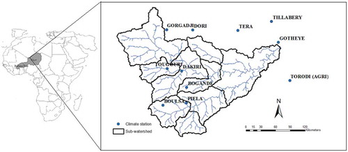
The Sirba watershed is a trans-boundary basin located between the countries of Niger and Burkina Faso (Fig. 2), at latitudes 12.2–14.5°N and longitudes 1.4°W–1.7°E. It has an area of approximately 37 000 km², most of which is in Burkina Faso. The basin is a sub-basin of the Middle Niger basin, and its three main tributaries, the Faga, Yeli and Sirba, originate in Burkina Faso and discharge into the Niger River at Garbe-Kourou in Niger. The Sirba River is an important tributary of the Niger River in the integrated area of southwestern Niger, eastern Burkina Faso and northern Mali.

Figure 2. Climate stations and sub-watersheds in the Sirba watershed.

More than half (53%) of the watershed is savannah, pasture and cropland cover approximately 23% each, and the remaining 1% is made up of sparse vegetation, shrub land and water. The USGS Global Land Cover Characterization (GLCC) database was the source of land-use data for the Sirba watershed (the map is available at http://www.waterbase.org.), and the Food and Agriculture Organization of the United Nations (FAO) provided soil data for the region as a base at a nominal scale of 1:5 000 000. There is no variability in soil type, as soil data are global and have a low spatial resolution. The entire basin is sand-loam soil of 60% sand, 30% silt and 10% clay. Descroix et al. (2009) summarized the hydrological data of this basin, as shown in Table 1.

2.2 Data

2.2.1 Precipitation and streamflow observations

The daily precipitation data were obtained from local climate stations, and prepared by the Nigerian and Burkina Faso meteorological services. Though there are many stations in and around the Sirba basin, only the daily precipitation datasets from climate stations with less than 10% missing data over the full observation period were selected for this study. Eleven precipitation time series from 1960 to 2006 were used, and the Thiessen polygon method was applied to estimate the average rainfall over the watershed. Figure 2 shows the locations of the climate stations inside and near the basin.

For the period 1962–2002, 41 years of daily streamflow observations at the Garbe-Korou station in Niger were obtained from the Nigerian Ministry of Hydraulics. The station is located at latitude 13°44ʹN and longitude 1°36ʹE. High flows typically occurred from July to September (the summer rainfall season), and low flows at the beginning of the year to June, and at year end. The average flow during July–September was 86 ± 56 m³/s (mean ± standard deviation), and the highest and lowest discharges for the period were 235 m³/s in 1998 and 7 m³/s in 1968. The first and third quartiles of the annual streamflow data were 49 and 114 m³/s, respectively.

2.2.2 Sea-surface temperature (SST)

The monthly Atlantic SST up to 18 months prior to the date of the forecasts was used as predictor in both approaches, as it had proved effective for streamflow forecasting in the Sirba watershed (Sittichok et al. 2016). The Atlantic SST data were obtained from the Meteorology and Water Resource Center of Ceara State, Brazil, and downloaded from the International Research Institute for Climate and Society website (http://iri.columbia.edu/). The dataset covers the period from 1964 to 2010, and consists of 25 points on the y-axis (latitudes 19°S–29°N) and 38 points on the x-axis (longitudes 59°W–15°E). Since the best period was not known in advance, the SST data were aggregated over various periods with different lengths and start dates. All periods started at the beginning of a calendar month, and ended at the end of a calendar month. The beginning of a period had to be later than or equal to 1 January of the previous year (i.e. Y – 1, where Y is the year with the rainy season for which the forecast was issued), and the end of the period had to be prior or equal to 30 June of year Y. Figure 3 demonstrates how all 171 periods that met these criteria were systematically arranged. The upper bar indicates all the months from January of the previous year (Y – 1) to June of the year the forecast was issued (Y). For example, in the first run only the SST of January (Y – 1) was selected as a predictor. The SST average over January and February (Y – 1) was used as a predictor in the second run, and this process was repeated at 1-month intervals until the end of the period, June (Y), was reached. Then the SST of February (Y – 1) was used as a predictor, followed by the SST average over February and March (Y – 1). The process was repeated until only the SST of June (Y) was used.

Figure 3. SST averaging periods.

3 Methodology

This study used both direct and indirect methods for streamflow forecasting. The direct method started with building multiple linear regressions between SST and annual streamflow during the rainy season (July–September: JAS) in the watershed. The fragment method developed by Harms and Campbell (1967) was used to convert forecast annual streamflow (JAS) into monthly streamflow. The proposed multi-statistical techniques combination specifically filtered only potential predictors at the first step before the use of principal component analysis (PCA) to reduce remaining predictors. Additionally, instead of arbitrarily selecting the periods of the predictor used for forecasting, as in other studies (Barnston et al. 1996, Fontaine et al. 1999, Lodoun et al. 2013), this study attempted to use all aggregated periods of predictor up to 18 months in advance to seek the best period.

The indirect method used the same techniques as the direct method to forecast annual rainfall during the rainy season (JAS), then the fragment method was used to generate daily rainfall before the SWAT model was applied to perform the rainfall–runoff transformation. The accuracy of the forecasts with each method was assessed using the coefficient of determination (R²), the Nash-Sutcliffe coefficient (E_f) and the Hit score (H). In addition, this research not only focused on the accuracy of forecasts but also evaluated economic values of forecasts using a simple cost/loss ratio (C/L). Analysis of the value of each method for different C/L situations provided criteria that could help decision makers select the most appropriate seasonal forecasting model for the configuration of the area under their authority.

3.1 Seasonal precipitation (indirect methods) and seasonal streamflow (direct methods) forecasting

Precipitation forecasts during the rainy season (JAS) (indirect methods) and streamflow forecasts during the rainy season (JAS) (direct methods) were generated following the methodology outlined in Sittichok et al. (2016). A 1-year cross-validation method was used for both precipitation forecasting (indirect methods) and streamflow forecasting (direct methods) to remove the forecast year from the dataset before constructing an empirical equation. The methodology is briefly discussed in the next three subsections. Details of all steps are indicated in Sittichok et al. (2016).

3.1.1 Search for the optimal lag time and optimal period to average the predictor

In this process the SSTs were aggregated over various periods prior to the date of the forecasts (indirect method for precipitation forecasts and direct method for streamflow forecasts). For each period for which the SSTs were aggregated, a cross-validation method was applied to remove a forecast year. The dimensions of the SST dataset were reduced to obtain a small number of predictors using statistical methods (details in the next section). Finally, a linear regression model was fitted to the remaining SST and precipitation/streamflow time series. The fitted linear regression was used to simulate the precipitation/streamflow for the forecast year that was removed at the beginning of the process. When a forecast precipitation/streamflow was available for each year in the historical period, R², E_f and H were used to estimate the model performance. Since there were 171 periods for SST, only the period that gave the highest E_f was presented.

3.1.2 SST vector dimension reduction methods

To reduce the dimensions of the SST dataset, a linear regression was fitted to the SST of a grid cell and the precipitation/streamflow to generate an empirical equation for calculation of precipitation/streamflow for forecast year Y. The linear regression was used to produce a simulated precipitation/streamflow series on the watershed and the E_f or R² value was calculated using the observed and simulated precipitation/streamflow series. If E_f was used to assess simulated and observed precipitation/streamflow, all grid cells were ranked high to low by E_f results. If R² was applied, only grid cells showing p values less than 0.05 were retained to use in the next step, and these were also ranked from high to low. The number of remaining grid cells forced to PCA depended on the specific value called NMAX. NMAX ranged from 10 to 200 with 10 increments, and was defined at the first step of the model. It helped to reduce the number of predictors in the process of PCA, and principal components (PCs) were then generated. Stepwise regression was applied in order to identify and retain only those PCs with predictive power.

In summary, two statistical methods for seasonal forecasting were used. In the first method (called Model I), R² was used as a criterion to obtain SST grid cells with high correlations to local precipitation/streamflow. Afterwards, PCA, stepwise regression and linear regression were applied. In the second method (called Model II), E_f was used instead of R² in order to discard predictors showing low relationships with local precipitation/streamflow. After using E_f, PCA, stepwise regression and linear regression were also applied.

3.1.3 Generation of a probabilistic forecast for precipitation (indirect method) and streamflow (direct method)

The methods described in the previous sections provide a deterministic forecast for each year, as well as a time series of residuals (errors). The forecasts were assumed to follow a normal distribution, with the mean as the estimate of the seasonal forecasting model and the standard deviation as the standard deviation of the residuals. This assumption allowed calculation of n equiprobable values of the total precipitation, by taking n annual precipitation values with exceedence probabilities of 1/2n, 3/2n, …, (2n − 1)/2n, given the probability distribution of the forecast annual precipitation, which was assumed to follow a normal distribution.

3.2 Temporal disaggregation

3.2.1 Precipitation disaggregation from annual to daily time scale

The SWAT model requires precipitation at the daily or sub-daily time scale. Therefore, it is necessary to disaggregate the forecast annual precipitation (JAS) from the previous step into daily data. In this study, the fragment method, first proposed by Harms and Campbell (1967) and continuously developed since (Porter and Pink 1991, Wójcik and Buishand 2003, Pui et al. 2009), was applied to increase the time scale of variables using the standardized historical data to generate the fragment series for each year. The challenge with this method is selecting the set of fragments that are multiplied with the annual forecast precipitations in order to expand the temporal scale. In this paper, the sets of fragments were obtained by the following steps:

1. The average annual precipitation observation during the rainy season (July–September) over the 11 stations was calculated using a Thiessen polygon technique, which is the basic method of calculating the average precipitation of an area (Chow et al. 1988).

2. For each year of forecast annual precipitation (FP_ai) in the series of forecast precipitation:

3. The year of historical annual precipitation (generated in the previous step) except year i with the average annual precipitation observation (OP_aj) closest to the annual forecast precipitation was selected.

4. The forecast daily precipitation at station k (FP_di__k) was estimated using the daily precipitation observations of station k (OP_{dj_k}) (Equation (1)), which generated the precipitation time series for nine stations while maintaining the rainfall distribution over the whole basin.

(1)

3.2.2 Streamflow disaggregation from annual to monthly streamflow

Streamflow forecasts generated using direct methods resulted in annual time scale for a rainy season (JAS). The time scale of forecast results was disaggregated to monthly data to be able to compare to streamflow forecasts generated using indirect methods (the SWAT model). The fragment method was applied for this purpose. The steps of streamflow disaggregation were as follows:

1. Monthly streamflow observations were aggregated over July–September for the entire period.

2. For each year of forecast annual streamflow (FF_ai) in the series of forecast streamflow:

   1. All aggregated observations except year i were calculated to find the difference in annual streamflow forecast (FF_ai). The results were sorted from lowest to highest. The observation year that presented the lowest result obtained from calculation was selected (called OF_aj).

   2. The monthly forecast streamflows of year i (FF_mi) were generated using monthly streamflow observations of year j (OF_mj) as:

      (2)

3.3 Rainfall–runoff modelling using SWAT

The Soil and Water Assessment Tool (SWAT), developed at the US Department of Agriculture, Agriculture Research Service (ARS), was used for rainfall–runoff transformation in this study. It is a physically-based model commonly applied to simulate river flows on daily and monthly time scales in various regions (Tripathi et al. 2004, Demirel et al. 2009, Huang et al. 2009, Xu et al. 2009).

The Sirba watershed model consists of nine sub-watersheds, five dams and nine reaches. The SWAT model generated 34 hydrological response units (HRUs). The SWAT model worked with the available climate data including temperature, radiation, wind speed, relative humidity and observed daily precipitation from 1989 to 2002. SWAT had approximately 240 parameters with different degrees of spatial variability. A sensitivity analysis performed using the Sequential Uncertainty Fitting algorithm in the SWAT Calibration and Uncertainty Program (SWAT-CUP), identified the 10 parameters with the strongest influence on streamflow (see Table 2). Streamflow data were available for a 14-year period (1989–2002) and the calibration and validation processes were performed using 1989–1995 and 1996–2002 datasets, respectively. The calibration performance was evaluated using the values of E_f, R² and H applied to monthly flow time series at the watershed outlet. Good performance was achieved for the calibration period, with R² = 0.95, E_f = 0.90 and H = 73%, and the model performance decreased in the validation period, with R² = 0.66, E_f = 0.60 and H = 79%.

Table 1. Main data for the hydrological regime in the Sirba basin (Descroix et al., 2009).

Parameter	Data
Mean discharge (m^3 s^−1)/Mean specific discharge (L s^−1 km^−2) (1950–2007)	24.5/38 750
Area (km^2)	0.63
Mean rainfall depth (mm/year) (1950–2007)	18.3
Latitude of basin	12.2–14.5°N
Longitude of basin	1.4°W–1.7°E

Table 2. The 10 most sensitive parameters of the SWAT model for streamflows in the Sirba watershed.

Parameter description	Variable name in the SWAT model	Range
Moisture condition II curve number (-)	CN2	20–90
Soil evaporation compensation coefficient (-)	ESCO	0.01–1
Available water capacity of the soil layer	SOL_AWC	0–1
Depth from soil surface to bottom of layer (mm)	SOL_Z	0–3500
Threshold water level in shallow aquifer for baseflow (mm H2O)	GWQMN	0–5000
Effective hydraulic conductivity (mm/h)	CH_K2	0–150
Maximum canopy storage (mm)	CANMX	0–100
Threshold depth of water in the shallow aquifer for “revap” to occur (mm)	REVAPMN	0–500
Potential maximum leaf area index for plants (-)	BLAI	0–12
Surface runoff lag coefficient (-)	SURLAG	1–24

3.4 Streamflow forecasting using the direct and indirect methods

As previously explained, direct and indirect streamflow forecasting methods were applied in this paper. These are summarized below:

1. The direct method involved (i) development of a seasonal streamflow forecasting method, (ii) generation of 10 equiprobable values of streamflow forecasts, and (iii) temporal disaggregation of each of the 10 streamflow values to the monthly scale. The final result was 10 equiprobable sets of monthly streamflow values, from 1989 to 2002.

2. The indirect method involved (i) development of a seasonal precipitation forecasting method, (ii) generation of 10 equiprobable values of precipitation forecasts, (iii) temporal disaggregation of each seasonal precipitation to the daily scale, (iv) application of the SWAT model to convert all daily precipitations to daily streamflows with all other SWAT inputs set to climatology, and (v) aggregation to the monthly time scale. The final result was 10 equiprobable sets of monthly streamflow values, from 1989 to 2002.

3.5 Model performance evaluation

Numerous criteria are applied to estimate model performance. The two criteria most widely used to evaluate climate and hydrological forecasting schemes are the coefficient of determination (R²) and the Nash-Sutcliffe coefficient (E_f) (Krause et al. 2005, Arnold et al. 2012).

The coefficient of determination, R², is traditionally used to measure the fit of a regression equation to observations (O) and model predictions (P). It can determine the proportion of variation of measurement data described or accounted for by the regression. Equation (3) shows the general form of R², where , and n are the average of observations, the average of predictions and the number of observations in a dataset, respectively. The value of R² is equal to 1 for a perfect model and zero for an unsuccessful model, zero indicating no variation in the observation that can be explained by the prediction.

(3)

The coefficient of efficiency, E_f, first proposed by Nash and Sutcliffe (1970), is an alternative criterion of model performance. It is used to determine the relative magnitude of the residual variance and the observation variance (Moriasi et al 2007). Equation (4) shows the formula to compute E_f, the value of which ranges from −∞ to 1, with 1 being a perfect model. An E_f ≤ 0 indicates that the mean of the observations should be used, rather than the simulated data (Moriasi et al. 2007).

(4)

The above two criteria are used for evaluating model performance with continuous data. However, both have drawbacks, as they rely on the variance of measured data and outliers, which could lead to incorrect conclusions regarding a model’s capability. Thus, this study also evaluates model performance with the Hit score (H), by converting observed and forecast streamflow into three categories: below normal, normal and above normal. H can vary from 0 to 100%, with a high value of H indicating good model performance. The equation used to calculate H is Equation (5), where r, v and z are the numbers of simulations falling in the same category of observations for all three categories: below normal, normal and above normal, respectively, and n is the number of observations in a dataset:

(5)

3.6 Forecast economic value estimation using the cost/loss ratio method

When the forecast information successfully leads to applicable actions, decision makers gain the highest benefits (Lee and Lee 2007). The cost/loss ratio method, first proposed by Thompson (1952), is a simple technique to determine the economic value of a forecast. It has been widely used to evaluate the economic value of weather and hydrological forecasting systems (Palmer 2002, Lee and Lee 2007, Rouline 2007, Millner 2009, Tena and Gomez 2011), and helps decision makers assess whether a protective action costing C should be implemented to prevent a loss L if a particular adverse event occurs. It is a simplification of the reality, however, since it assumes that the adverse event can be described by a categorical variable (occurrence/no occurrence), and that a single value of loss can be associated with that event (e.g. water levels exceeding the height of a protection dyke). The value of a forecasting system is estimated using:

(6)

where V is the economic value of the forecast system, determined by the ratio of the reduction in mean expense to the reduction in expense when perfect forecasts are accessible (Richardson 2012). The value of can be obtained by considering the minimum cost of a protective action (C), or by multiplying the climatological base rate probability (s) and the expense of loss (L) for each event []. The is calculated in terms of the likelihood of the base rate probabilities [], and F is the false alarm from the contingency table. Finally, is the mean expense if the action were taken when the extreme event was going to occur [] (Richardson 2012). Given that the cost/loss ratio is not known and is likely to change with time, V was estimated for C/L ratios ranging from 0 to 1. The upper limit for C/L is 1, because decision makers would not take protective action if the cost of protection were greater than the potential loss (Richardson 2012). To illustrate the methodology, three monthly discharges with 2-, 5- and 10-year return periods were used as adverse events in this study.

The economic values of monthly forecast streamflows generated using direct and indirect methods were estimated using the cost/loss ratio method. In the first step, 10 different probability distributions – generalized extreme value (GEV), Pearson Type III, two- and three-parameter lognormal models, generalized logistic, extreme value, generalized Pareto, normal, exponential normal, logistic and gamma – were tested to seek the suitable distribution fitting the time series of monthly maximum flows of the Sirba basin. The extreme flows of 2-, 5- and 10-year return periods were then calculated. Finally, forecast streamflows were converted into categorical data, and contingency tables for each forecasting method and each return period were developed.

4 Results

The optimal parameters of the two methods, their performance in terms of rainfall and/or streamflow forecasting and economic value are discussed herein.

4.1 Direct method

A total of 6840 streamflow forecasts were generated, using 171 aggregated Atlantic SST periods as predictors with different NMAX. Both statistical models developed the best forecasts from the same SST averaging period of June of the previous year. Thus, it seemed that the Atlantic SST in June of the year before forecasts were issued was the most suitable period for streamflow forecasting in the Sirba basin. The best forecast was generated using Model II, with a reasonable performance of R² = 0.43, E_f = 0.42 and H = 43%, with NMAX of 200. The Atlantic SST dimension decreased from 950 to 200 points using E_f at the first step, and all the remaining data were used in PCA. The first PC showed a maximum percentage of explained variance of approximately 41%. The Model I performance of R² = 0.35, E_f = 0.34 and H = 35% was insignificantly less than that of Model II when R² and E_f were used for estimation (Table 3). However, noticeable differences between the models were indicated by the H values, which showed that forecasts from Model II were more often in the same categories as the observations than forecasts from Model I.

Table 3. Performance of statistical models I and II for seasonal precipitation and streamflow forecasting.

	Period	NMAX	R^2	Ef	H
Streamflow forecasting
Model I	June (Y – 1)	170	0.35	0.34	35
Model II	June (Y – 1)	200	0.43	0.42	43
Rainfall forecasting
Model I	Sep.–Dec. (Y – 1)	50	0.29	0.23	48
Model II	Jul.–Jan. (Y)	180	0.14	0.13	48

After increasing the time scale of the best forecast from annual to monthly data using the fragment method, a value of 0.61 was obtained for R², and E_f and H reached 0.54 and 82% respectively (Table 4). Peak flow overestimations in 1989, 1990 and 2001 are evident in Figure 4, whereas peak flows were underestimated in 1991, 1992 and 1994. As the forecast was issued 12 months before the rainy season, these moderate forecasting skills were expected.

Table 4. Comparison of the performance of direct and indirect methods for streamflow forecasting. Bold indicates best performance.

Time scale	Method	Period	Lead time	NMAX	R^2	Ef	H
Monthly	Direct method	June (Y – 1)	12	200	0.61	0.54	82
	Indirect method	Sep.–Dec. (Y – 1)	6	–	0.70	0.69	77
Annual	Direct method	June (Y – 1)	12	200	0.43	0.42	43
	Indirect method	Sep.–Dec. (Y – 1)	6	–	0.0003	–0.06	43

Figure 4. Comparison between observations and streamflow forecasts using direct and indirect methods (SWAT model).

4.2 Indirect method

Results of the indirect method are described in the three subsections below.

4.2.1 Rainfall forecasting

The SST aggregated over September–December of the previous year was found to be the best predictor for seasonal precipitation forecasting, and the best simulated precipitation was developed using Model I with R² as the criterion in the first step. Fifty SST grid data points (NMAX = 50) were used in the PCA, and the variance of the first PC indicated that approximately 80% had R² = 0.29, E_f = 0.23 and H = 48% (Table 3). Model I showed insignificantly better performance than Model II with respect to H, but remarkable differences in E_f and R². The simulated and observed annual precipitation forecasts for the rainy season (JAS) are presented in Figure 5. The indirect forecasting method was able to capture the general trend of the observation time series, but failed to obtain the highest and the lowest precipitation, with the exception of 1965. These results show that using the different methods to specifically filter powerful SST grid data (Model I with R² and Model II with E_f) affects the skill of the rainfall forecasting method.

Figure 5. Comparison between observed annual precipitation and forecast precipitation using models I and II.

4.2.2 Temporal disaggregation of rainfall forecasts

Precipitation forecasts successfully generated using Model I were disaggregated to the daily time step, so they could be used to drive the SWAT model. The performance values of monthly precipitation (aggregated from daily data) were R² = 0.8, E_f = 0.81 and H = 87%, obtained when the disaggregated time series were compared to the observations.

4.2.3 Rainfall–runoff transformation

The three most sensitive parameters influencing the model’s capability were moisture condition II curve number (CN2), soil evaporation compensation coefficient (ESCO) and available water capacity of the soil layer (SOL_AWC). Depending on the sub-basin and HRU, CN2 varied from 60 to 75, and the ESCO and SOL_AWC values were 0.9. After the model was calibrated, the best values of the sensitive parameters were used to generate river flow forecasts. Daily rainfalls developed in the previous section were introduced as input layers to the SWAT model, and monthly flows from 1989 to 2002 were forecast. The model performance results were R² = 0.70, E_f = 0.69 and H = 77% (Table 4).

4.3 Comparison of the performance of direct and indirect methods for streamflow forecasting

Deterministic forecasts obtained using the direct and indirect methods are shown in Figure 4. Both models successfully generated streamflow forecasts in terms of trends and data patterns, and both occasionally led to flow overestimation and underestimation in both high- and low-flow seasons. On the monthly time scale, the indirect method (R² = 0.70, E_f = 0.69) performed better than the direct method (R² = 0.61, E_f = 0.54), but the indirect method had a lower hit score (see Table 4). However, on the annual time scale for the rainy season (JAS), the direct method (R² = 0.43, E_f = 0.42) significantly outperformed the indirect method, which showed a negative E_f and R² close to zero; both had the same hit score. These results suggest that the indirect method is better able to capture intra-seasonal variations, and the direct method is more effective for capturing inter-annual variations. The use of the SWAT model in the indirect method led to more realistic hydrographs, because SWAT accounts explicitly for the physical processes that generate streamflow at the basin level. However, the use of SWAT has higher data and computation requirements. Thus, in addition to describing inter-annual variability better, the direct method also requires less data, and has a longer forecast lead time of 12 months.

Figure 6 shows the lower and upper ranges of streamflow forecasts for each approach, as well as the observations. The observations fell in the lower and upper ranges of the direct and indirect methods around 77 and 60%, and the highest differences between lower and upper ranges were 306 and 277 m³/s, respectively. Overall, the observations were inside the forecast range, except in 1990, 1991 and 1994. High overestimation and underestimation occurred in 1990 and 1994, while different peak times between observations and streamflow forecasts were observed in 1991 in both simulations.

Figure 6. Lower and upper ranges of streamflow forecasts: (a) direct method and (b) indirect method.

4.4 Economic value of streamflow forecasting

To evaluate the economic value of streamflow forecasts, monthly maximum forecast streamflow time series were tested with 10 different probability distributions: GEV, Pearson Type III, two- and three-parameter lognormal models, generalized logistic, extreme value, generalized Pareto, normal, exponential normal, logistic and gamma. The results showed that GEV was the best fit. The extreme flows of 2-, 5- and 10-year return periods were 117, 192 and 243 m³/s, respectively. For each of these flow values, the forecast streamflows were converted to categorical data (i.e. flood/no flood). Contingency tables for each forecasting method and return period are presented in Table 5. A total of 1441 events was used to generate the contingency tables, and higher agreement was found with an increased number of return periods in both methods. With the direct method, the SWAT model resulted in more underestimations and fewer overestimations. Note that probabilistic forecast values were used, which led to 10 forecasts and one observation for each year, each return period and each forecasting method. False alarms (F), Hit rates (H) and base rates (s) were computed based on the values in the contingency tables. Forecast values were calculated for C/L ratios ranging from 0 to 1 at increments of 0.2, and are shown in Figure 7 for all return periods. The value of the forecast information based on both methods had a wide cost/loss ratio of 0.2–1 for 2-year return periods. The value increased until the C/L ratios were in the 0.8–0.9 range, then decreased to zero when the C/L ratio was 1.

Table 5. Contingency tables of streamflow forecasting using direct and indirect methods based on 2-, 5- and 10-year return periods.

	Indirect method
Direct method	Observations					Observations
2-year return period
		≤117	>117				≤117	>117
Forecasts	≤117	1238	65	1303	Forecasts	≤117	1241	77	1318
	>117	38	100	138		>117	35	88	123
		1276	165	1441			1276	165	1441
5-year return period
		≤192	>192				≤192	>192
Forecasts	≤192	1356	33	1389	Forecasts	≤192	1370	48	1418
	>192	30	22	52		>192	16	7	23
		1386	55	1441			1386	55	1441
10-year return period
		≤243	>243				≤243	>243
Forecasts	≤243	1383	24	1407	Forecasts	≤243	1403	30	1433
	>243	25	9	34		>243	5	3	8
		1386	33	1441			1386	33	1441

Figure 7. Economic values based on adverse events: 2-, 5- and 10-year return periods.

It was determined that the direct method had higher values than the indirect method for return periods of 2 and 5 years, and for C/L ratios above 0.7 when the return period was 10 years. The differences in forecast values between the two methods were insignificant when the return period was 2 years, and significant for higher return periods. For example, for the Sirba watershed when the C/L ratio was 0.9, the forecast value of the direct method was higher than 0.3, while the indirect method was 0.1 for a 5-year return period. The value of forecasts declined with higher return periods for both methods. The results indicate that for the Sirba watershed the direct method provided better information for flood protection, and thus it should be recommended. In situations where the shape of the hydrograph is important (e.g. irrigation planning), the indirect method could provide additional information. However, to use this information for decision making in water resources management, decision makers should also consider other aspects such as social and livelihood points of view.

5 Discussion

The two statistical models (direct and indirect methods) were applied to forecast precipitation and streamflow a few months in advance. For direct methods streamflow was forecast directly, using SST, whereas for indirect methods, precipitation was forecast first, then translated into streamflow using the SWAT model. Surprisingly, both models showed slightly better performance in predicting monthly streamflow than monthly precipitation. This could be because precipitation to streamflow transformation is highly nonlinear, and therefore the best performance in precipitation forecasting (as measured using E_f) does not necessarily translate into the best E_f in streamflow forecasting. It also shows that E_f does not perfectly capture the match between simulated and observed variables.

Both the direct and indirect seasonal forecasting approaches developed in this paper could skilfully forecast streamflow in the Sirba watershed, which is a sub-basin of the Niger River basin (the main basin of the Sahel region), using the Atlantic SST. The direct method outperformed the indirect method on the annual time scale, as it better reproduced inter-annual variability. However, the indirect method showed higher performance on the monthly time scale, and was therefore better at capturing intra-seasonal variability. The indirect method also has the advantage of using rainfall–runoff transformation, which could lead to more realistic hydrographs because generating the transformation takes physical processes into account.

The benefits of using statistical models for seasonal forecasting were highlighted in this study. However, these models are data driven, and do not necessarily mimic the physical mechanisms behind the correlations between independent and dependent variables. Such models are strongly sensitive to the quality of the input data forced into them, and using the same type of predictor datasets with different methodologies could lead to different outputs in terms of forecast accuracy, lead time and model efficiency. Using statistical models requires assuming that the relationship between the predictors and the predictand is stable, and that the modelled process will behave in the future as it has in the past; nonstationary data could cause forecasting errors (Ionita et al. 2008, 2014). Therefore, testing the statistical models to determine the optimum predictor periods when updated data are available, before using them to forecast rainfall or streamflows, is strongly recommended. The performance of statistical models could also decrease when the historical data of both the predictors and the predictand is not adequate to determine their relationships, there are too many gaps in the datasets, or the selected predictor pool has a weak or instable correlation with the predictand. However, these issues can be solved by using sophisticated methods, combining forecasts from multiple models or multi-model ensemble combination techniques (Block et al. 2009, Wang and Robertson 2011, Wang et al. 2012).

The economic value of the simulated monthly streamflows generated with the direct method was relatively higher than of those produced by the indirect method for all return periods, which could be due to the method used to determine the economic value. The ratio method is based on converting continuous data to categorical data that are consistent with an estimator’s hit score. The simulated flows generated with the direct method also showed higher hit score values than the indirect method, which highlights the need to select model performance criteria in hydrological studies carefully. In this study, the method with a lower E_f proved to have the highest economic value. Thus, if the traditional approach of discarding models based on their E_f had been applied, the model with the highest economic value would have been discarded.

In this study, linear relationships between SST and precipitation/streamflow were assumed. However, to improve seasonal forecasting skills in future work, the potentially nonlinear nature of these relationships should also be considered. In addition, SSTs are only one potentially useful predictor of precipitation and streamflow forecasting. Other atmospheric and oceanic variables such as mean sea-level pressure, ENSO index and wind velocity could also be considered.

6 Conclusions

The performance of direct and indirect seasonal streamflow forecasting methods applied on the Sirba watershed (West Africa) was compared in terms of their accuracy and economic value. The direct method used a linear relationship to relate sea surface temperature (SST) to annual streamflow in the rainy season (JAS), after which the data were disaggregated on the monthly time scale. The indirect method used a linear relationship to generate annual precipitation (JAS) on the watershed, a temporal disaggregation step to generate daily precipitation, and the SWAT (Soil and Water Assessment Tool) model to generate monthly streamflow hydrographs. The economic benefits were estimated using the cost/loss ratio method. It was determined that the direct method is more capable of capturing inter-annual variations, while the indirect method provides a better description of intra-seasonal variations for the Sirba basin. Despite its lower data requirements and computational effort, the economic value of the direct method was found to be higher; it therefore provided more valuable information for flood protection in the watershed.

Acknowledgements

The authors thank the International Development Research Center (Canada) and the National Science and Engineering Research Council of Canada for funding this research.

Disclosure statement

No potential conflict of interest was reported by the authors.

Additional information

Funding

This work was supported by the National Science and Engineering Research Council of Canada and the International Development Research Center Canada.

References

- Abedokun, J.A., 1979. Towards achieving an in-season forecasting of the west African precipitation. Archive for Meteorology. Geophysics and Bioclimatology Series A, 28, 19–38. doi:10.1007/BF02316315
- Abudu, S., King, J.P., and Pagano, T.C., 2010. Application of partial least-square regression in seasonal streamflow forecasting. Journal of Hydrologic Engineering, 15, 612–623. doi:10.1061/(ASCE)HE.1943-5584.0000216
- Arnold, J.G., et al., 2012. SWAT: model use, calibration, and validation. American Society of Agriculture and Biological Engineers, 55, 1491–1508.
- Barnston, A.G., Thiao, W., and Kumar, V., 1996. Long-lead forecasts of seasonal precipitation in Africa using CCA. Weather and Forecasting, 11, 506–520. doi:10.1175/1520-0434(1996)011<0506:LLFOSP>2.0.CO;2
- Biasutti, M., et al., 2008. SST Forcings and Sahel rainfall variability in simulations of the Twentieth and Twenty-First centuries. Journal of Climate, 21, 3471–3486. doi:10.1175/2007JCLI1896.1
- Block, P.J., et al., 2009. A streamflow forecasting framework using multiple climate and hydrological models. Journal of the American Water Resources Association, 45, 828–843. doi:10.1111/j.1752-1688.2009.00327.x
- Bouali, L., et al., 2008. Performance of DEMETER calibration for rainfall forecasting purposes: application to the July-August Sahelian rainfall. Journal of Geophysical Research, 113, 1–12. doi:10.1029/2007JD009403
- Brooks, N., 2004. Drought in the African Sahel: long term perspectives and future prospects. Tyndall Centre Working Paper, vol 61. Tyndall Centre for Climate Change Research, School of Environmental Sciences, University of East Anglia, Norwich.
- Chow, V., Maidment, D., and Mays, L., 1988. Applied hydrology. New York: McGraw-Hill Science.
- Day, J.C., Hughes, D.W., and Butcher, W.R., 1992. Soil, water and crop management alternatives in rainfed agriculture in the Sahel: an economic analysis. Agricultural Economics, 7, 267–287. doi:10.1016/0169-5150(92)90053-2
- Demirel, M.C., Venancio, A., and Kahya, E., 2009. Flow forecasts by SWAT model and ANN in Pracana basin, Portugal. Advanced in Engineering Software, 40, 467–473. doi:10.1016/j.advengsoft.2008.08.002
- Descroix, L., et al., 2009. Spatio-temporal variability of hydrological regimes around the boundaries between Sahelian and Sudanian areas of West Africa: a synthesis. Journal of Hydrology, 375, 90–102. doi:10.1016/j.jhydrol.2008.12.012
- Folland, C., et al., 1991. Prediction of seasonal rainfall in the Sahel region using empirical and dynamic models. Journal of Forecasting, 10, 21–56. doi:10.1002/for.3980100104
- Fontaine, B., Philippon, N., and Camberlin, P., 1999. An improvement of June-September rainfall forecasting in the Sahel based upon region April-May moist static energy content (1968-1997). Geophysical Research Letters, 26, 2041–2044. doi:10.1029/1999GL900495
- Garbrecht, J.D., Schneider, J.M., and Van Liew, M.W., 2007. Monthly runoff predictions based on rainfall forecasts in a small Oklahoma Watershed. Journal of the American Water Resources Association, 42, 1285–1295. doi:10.1111/j.1752-1688.2006.tb05301.x
- Garric, G., Douville, H., and Deque, M., 2002. Prospect for improved seasonal predictions of monsoon precipitations over the Sahel. International Journal of Climatology, 22, 331–345. doi:10.1002/joc.736
- Gneiting, T. and Raftery, A.E., 2005. Weather forecasting with ensemble methods. Science, 310, 248–249. doi:10.1126/science.1115255
- Gobena, A.K. and Gan, T.Y., 2010. Incorporation of seasonal climate forecasts in the ensemble streamflow prediction system. Journal of Hydrology, 385, 336–352. doi:10.1016/j.jhydrol.2010.03.002
- Harms, A.A. and Campbell, T.H., 1967. An extension to the Thomas-Fiering model for the sequential generation of streamflow. Water Resource Research, 3, 653–661. doi:10.1029/WR003i003p00653
- Hatzaki, M., et al., 2007. The eastern Mediterranean teleconnection pattern: identification and definition. International Journal of Climatology, 27, 727–737. doi:10.1002/joc.1429
- Huang, Z., Xue, B., and Pang, Y., 2009. Simulation on stream flow and nutrient loadings in Gucheng Lake, Low Yangtze River Basin, based on SWAT model. Quaternary International, 208, 109–115. doi:10.1016/j.quaint.2008.12.018
- Hunt, B.G., 2000. Natural climatic variability and Sahelian rainfall trends. Global and Planetary Change, 24, 107–131. doi:10.1016/S0921-8181(99)00064-8
- Ionita, M., et al., 2014. Predicting the June 2013 European flooding based on precipitation, soil moisture and sea level pressure. Journal of Hydrometeorology. doi:10.1175/JHM-D-14-0156.1
- Ionita, M., Lohmann, G., and Rimbu, N., 2008. Prediction of Elbe discharge based on stable teleconnections with winter global temperature precipitation. Journal of Climate, 21, 6215–6226. doi:10.1175/2008JCLI2248.1
- Janicot, S., Trzaska, S., and Poccard, I., 2001. Summer Sahel – ENSO teleconnection and decadal time scale SST variations. Climate Dynamics, 18, 303–320. doi:10.1007/s003820100172
- Kandji, S.T., Verchot, L., and Mackensen, J., 2006. Climate change and variability in the Sahel region: impacts and adaptation strategies in the agricultural sector. World Agroforestry Centre (ICRAF) and United Nations Environment Programme (UNEP).
- Karamouz, M. and Zahraie, B., 2004. Seasonal streamflow forecasting using snow budget and El Nino-Southern Oscillation climate signals: application to the Salt River basin in Arizona. Journal of Hydrologic Engineering, 9, 523–533. doi:10.1061/(ASCE)1084-0699(2004)9:6(523)
- Krause, P., Boyle, D.P., and Bäse, F., 2005. Comparison of different efficiency criteria for hydrological model assessment. Advances in Geosciences, 5, 89–97. doi:10.5194/adgeo-5-89-2005
- Kwon, H., et al., 2009. Seasonal and annual maximum streamflow forecasting using climate information: application to the Three Gorges Dam in the Yangtze River basin, China. Hydrological Science Journal, 54, 582–595. doi:10.1623/hysj.54.3.582
- Lee, K.K. and Lee, J.W., 2007. The economic value of weather forecasts for decision-making problems in the profit/loss situation. Meteorological Application, 14, 455–463. doi:10.1002/met.44
- Liu, Z. and Alexander, M., 2007. Atmospheric bridge, oceanic tunnel, and global climatic teleconnections. Reviews of Geophysics, 45, RG2005. doi:10.1029/2005RG000172
- Lodoun, T., et al., 2013. Seasonal forecasts in the Sahel region: the use of rainfall-based predictive variables. Theoretical and Applied Climatology. doi:10.1007/s00704-013-1002-1
- Lu, J. and Delworth, T.L., 2005. Oceanic forcing of the late 20th century Sahel drought. Geographic Research Letters, 32, 1–5. doi:10.1029/2005GL023316
- Millner, A., 2009. What is the true value of forecasts? Weather Climate and Society, 1, 22–37. doi:10.1175/2009WCAS1001.1
- Moriasi, D.N., et al., 2007. Model evaluation guidelines for systematic quantification of accuracy in watershed simulations. American Society of Agricultural and Biological Engi- Neers, 50, 885–900.
- Nash, J.E. and Sutcliffe, J.V., 1970. River flow forecasting through conceptual models, Part I – A discussion of principles. Journal of Hydrology, 10, 282–290. doi:10.1016/0022-1694(70)90255-6
- Ndiaye, O., Goddard, L., and Ward, M.N., 2009. Using regional wind fields to improve general circulation model forecasts of July-September Sahel rainfall. International Journal of Climatology, 29, 1262–1275. doi:10.1002/(ISSN)1097-0088
- Ndiaye, O., Ward, M.N., and Thiaw, W.M., 2011. Predictability of seasonal sahel rainfall using GCMs and lead-time improvements through the use of a coupled model. Journal of Climate, 24, 1931–1949. doi:10.1175/2010JCLI3557.1
- Nnaji, A.O., 2001. Forecasting seasonal rainfall for agricultural decision-making in northern Nigeria. Agricultural and Forest Meteorology, 107, 193–205. doi:10.1016/S0168-1923(00)00239-2
- Palmer, T.N., 2002. The economic value of ensemble forecasts as a tool for risk assessment: from days to decades. Quarterly Journal of the Royal Meteorological Society, 128, 747–774. doi:10.1256/0035900021643593
- Piechota, T.C., et al., 1998. Seasonal streamflow forecasting in eastern Australia and the El Niño-Southern Oscillation. Water Resources Research, 34, 3035–3044. doi:10.1029/98WR02406
- Porter, J.W. and Pink, B.J., 1991. A method of synthetic fragments for disaggregation in stochastic data generation. In: International Hydrology and Water Resources Symposium, Perth, Australia, 781–786.
- Pui, A., Sharma, A., and Mehrotra, R., 2009. A comparison of alternatives for daily to sub-daily rainfall disaggregation. In: 18th World IMACS/MODSIM Congress, 13–17 July 2009, Cairns, Australia.
- Richardson, D.S., 2012. Economic value and Skill. In: Forecast verification: a practitioner’s guide in atmospheric science. 2nd ed. Published online: 21 Feb 2012. doi:10.1002/9781119960003.ch9.
- Robertson, D.E., Pokhrel, P., and Wang, Q.J., 2013. Improving statistical forecasts of seasonal streamflows using hydrological model output. Hydrology and Earth System Sciences, 17, 579–593. doi:10.5194/hess-17-579-2013
- Rouline, E., 2007. Skill and relative economic value of medium-range hydrological ensemble predictions. Hydrology and Earth System Sciences, 11, 725–737. doi:10.5194/hess-11-725-2007
- Rowell, D.P., et al., 1992. Modelling the influence of global sea surface temperatures on the variability and predictability of seasonal Sahel rainfall. Geophysical Research Letters, 19, 905–908. doi:10.1029/92GL00939
- Samimi, C., Fink, A.H., and Paeth, H., 2012. The 2007 flood in the Sahel: causes, characteristics and its presentation in the media and FEWS NET. Natural Hazards and Earth System Science, 12, 313–325. doi:10.5194/nhess-12-313-2012
- Schepen, A., Wang, Q.J., and Robertson, D., 2012. Evidence for using lagged climate indices to forecast Australian seasonal rainfall. Journal of Climate, 25, 1230–1246. doi:10.1175/JCLI-D-11-00156.1
- Sittichok, K., et al., 2016. Statistical seasonal rainfall and streamflow forecasting for the Sirba watershed, using sea surface temperature. Hydrological Sciences Journal, 61, 805–815.
- Tena, E.C. and Gomez, S.Q., 2011. Economic value of weather forecasting: the role of risk aversion. TOP, 19, 130–149. doi:10.1007/s11750-009-0114-3
- Thiaw, W. and Mo, K.C., 2005. Impact of sea surface temperature and soil moisture on seasonal rainfall prediction over the Sahel. Journal of Climate, 18, 5330–5343. doi:10.1175/JCLI3552.1
- Thompson, J.C., 1952. On the operational deficiencies in categorical weather forecasts. Bulletin of the American Meteorological Society, 33, 223–226.
- Tripathi, M.P., et al., 2004. Hydrological modelling of a small watershed using generated rainfall in the soil and water assessment tool model. Hydrological Processes, 18, 1811–1821. doi:10.1002/hyp.1448
- Tuteja, N.K., et al., 2011. Experiment evaluation of the dynamic seasonal streamflow forecasting approach. Melbourne: Bureau of Meteorology, Technical Report.
- Wang, E., et al., 2011a. Monthly and seasonal streamflow forecasts using rainfall–runoff modelling and POAMA predictions. In: 19th International Congress on Modelling and Simulation, 12–16 December 2011, Perth, Australia.
- Wang, E., et al., 2011b. Monthly and seasonal streamflow forecasts using rainfall–runoff modeling and historical weather data. Water Resources Research, 47, W05516 (1–13). doi:10.1029/2010WR009922
- Wang, Q.J. and Robertson, D.E., 2011. Multisite probabilistic forecasting of seasonal flows for streams with zero value occurrences. Water Resources Research, 47, W02546. doi:10.1029/2010WR009333
- Wang, Q.J., Schepen, A., and Robertson, D.E., 2012. Merging seasonal rainfall forecasts from multiple statistical models through Bayesian model averaging. Journal of Climate, 25, 5524–5537. doi:10.1175/JCLI-D-11-00386.1
- Washington, R. and Downing, T.E., 1999. Seasonal forecasting of African rainfall: prediction, responses and household food security. The Geographical Journal, 165, 255–274. doi:10.2307/3060442
- Wójcik, R. and Buishand, T.A., 2003. Simulation of 6-hourly rainfall and temperature by two resampling schemes. Journal of Hydrology, 273, 69–80. doi:10.1016/S0022-1694(02)00355-4
- Xu, Z.X., et al., 2009. Assessment of runoff and sediment yield in the Miyun reservoir catchment by using SWAT model. Hydrological Processes, 23, 3619–3630. doi:10.1002/hyp.7475
- Yossef, N.C., et al., 2013. Skill of global seasonal streamflow forecasting system, relative roles of initial conditions and meteorological forcing. Water Resources Research, 49, 4687–4699. doi:10.1002/wrcr.20350