Prediction of streamflow regimes over large geographical areas: interpolated flow–duration curves for the Danube region

ABSTRACT

Flow–duration curves (FDCs) are essential to support decisions on water resources management, and their regionalization is fundamental for the assessment of ungauged basins. In comparison with calibrated rainfall–runoff models, statistical methods provide data-driven estimates representing a useful benchmark. The objective of this work is the interpolation of FDCs from ~500 discharge gauging stations in the Danube. To this aim we use total negative deviation top-kriging (TNDTK), as multi-regression models are shown to be unsuitable for representing FDCs across all durations and sites. TNDTK shows a high accuracy for the entire Danube region, with overall Nash-Sutcliffe efficiency values computed in a leave-p-out cross-validation scheme (p equal to one site, one-third and half of the sites), all above 0.88. A reliability measure based on kriging variance is attached to each interpolated FDC at ~4000 prediction nodes. The GIS layer of regionalized FDCs is made available for broader use in the region.

KEYWORDS:

• flow–duration curve
• total negative deviation top-kriging
• prediction in ungauged basins (PUB problem)
• geostatistics
• Danube region

Editor D. Koutsoyiannis Associate editor not assigned

1 Introduction

The increasing accessibility of global datasets on soil, land cover, morphology and weather forcing, and enhanced computing capacity have backed the development of regional-, continental- and global-scale rainfall–runoff simulation models over the past decade (see e.g. Collischonn et al. 2007, de Paiva et al. 2013, Bierkens et al. 2015). Progressively accurate, large-scale models provide a wealth of information for addressing a variety of water problems, such as the prediction of streamflow regime in data-scarce regions of the world (e.g. Pechlivanidis and Arheimer 2015) and the implementation of large-scale and trans-boundary policies for water resources system management (e.g. de Roo et al. 2012), or flood-risk mitigation (de Paiva et al. 2013, Sampson et al. 2015, Falter et al. 2016). However, the local performances are highly variable (see e.g. de Paiva et al. 2013, Donnelly et al. 2016), reflecting the quality of macroscale input data and the adequacy of the conceptual scheme to accurately represent peculiar hydrological processes that locally drive the rainfall–runoff transformation.

An empirical characterization of the natural streamflow regime over large areas could be used as a benchmark, although the availability and accessibility of streamflow observations can be limiting even in technologically advanced regions of the world. This study presents a statistical regionalization of streamflow regimes in the Danube region, which is the largest watershed in Europe.

For a compilation of 511 discharge measurement stations across the Danube river basin, streamflow indices and empirical period-of-record flow–duration curves (FDCs) were computed along with a set of catchment descriptors. An FDC represents the probability for a given river cross-section of streamflow being greater than or equal to a given discharge value; as such an FDC is a hydrological signature of a given catchment and its shape reflects climate conditions and the hydrogeological characteristics of the catchment itself (see e.g. Castellarin 2014, Westerberg et al. 2016). For this reason, FDCs are routinely used for addressing water resources management problems such as hydropower feasibility studies, classification of streamflow regimes, design of water supply systems, irrigation planning and management, definition of environmental flows, habitat suitability studies, etc. (see e.g. Vogel and Fennessey 1995, Yaeger et al. 2012).

We first conducted a comprehensive exploration of the relationships between streamflow regime descriptors and the characteristics of basins. The identified relationships were used to develop multi-regression models for predicting the streamflow indices of interest and for quantifying their predictive accuracy.

Subsequently, we interpolated the streamflow regime over the whole Danube river basin, using the recently proposed geostatistical procedure termed total negative deviation top-kriging (TNDTK; Pugliese et al. 2014). Compared to regional regression models (see e.g. Blöschl et al. 2013), the accuracy of which is generally unsatisfactory for large and highly heterogeneous study regions, geostatistical procedures have been shown to provide highly reliable predictions of streamflow indices over large study areas, such as FDCs (see e.g. Pugliese et al. 2016), low flows (see e.g. Castiglioni et al. 2011, Parajka et al. 2015), flood flows (see e.g. Archfield et al. 2013), or the entire streamflow regime (see e.g. Farmer 2016).

This contribution illustrates the performance of a TNDTK geostatistical interpolation of the empirical FDCs in the Danube region and discusses the uncertainty of the interpolation.

2 Study area and database description

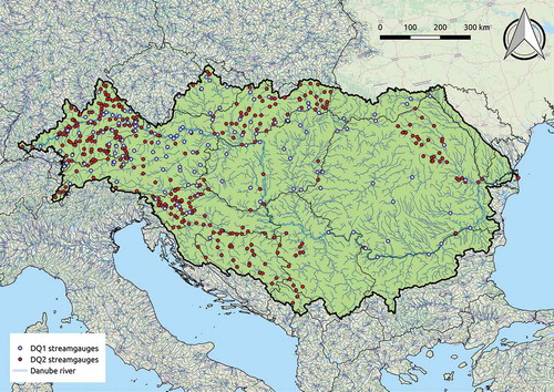
The present study uses a database compiled by the Joint Research Centre of the European Commission (DG JRC), consisting of 511 streamgauges across the Danube Basin (see Fig. 1). Streamflow indices (mean annual flow, MAF, and 15 streamflow quantiles associated with durations of 1, 5, 10, 20, 30, 40, 50, 60, 70, 75, 80, 90, 95, 97 and 99.7%) were computed from the time series of streamflow at each gauge, together with a set of catchment descriptors. The streamflow data quality has been classified as high quality (DQ1, blue open circles in Fig. 1) and lower quality (DQ2, red solid dots in Fig. 1): DQ1 refers to gauging stations with a precise positioning along the stream that are unique in their elementary sub-basin (i.e. portion of basin directly drained by a river stretch, between two confluences, or from the headwater to the first confluence), whereas DQ2 refers to cases in which more streamgauges are present in a single elementary basin, hence potentially affected by imprecise positioning along the stream. Together with the above-mentioned streamgauges, the DG JRC identifies 4381 prediction nodes over the Danube region, for which we performed the prediction of FDCs described herein.

Figure 1. Streamgauges considered in this study. Total of 511 streamgauges; blue open circles: high-quality data (DQ1, 138 gauges); red solid dots: low-quality data (DQ2, 373 gauges).

We considered all catchment descriptors reported in the DG JRC database: basin area (km²); minimum, maximum and mean basin elevation (m a.s.l.); maximum and minimum average daily temperature (°C); mean annual precipitation (mm); mean annual potential evapotranspiration (mm); mean annual number of rainy days (-); population density for the years 1980, 1990, 2000 and 2015 (inhab km⁻²); mean of population densities (inhab km⁻²); fractions of Cropland, Grassland, Shrub, Bare Soil, Forest, Water, Urban, Fertilized Cropland and Fertilized Grassland within the total basin area (-). Table 1 summarizes the empirical values of a selection of streamflow indices and catchment descriptors for the 511 study catchments.

Table 1. Minimum, 25th percentile, median, mean, 75th percentile and maximum for a selection of streamflow indices and catchment descriptors of the 511 study basins. Streamflow indices: 95th, 50th and 1st percentiles in m³ s⁻¹ km²; FDC slope between 70th and 30th streamflow percentiles at logarithmic scale (see e.g. Yaeger et al. 2012) (-); TND: empirical total negative deviation (a metric of empirical FDCs shape as defined in Pugliese et al. 2014) (-). Catchment descriptors: basin area (km²); minimum maximum and mean basin elevation (m a.s.l.); average maximum and daily temperature (°C); mean annual precipitation (Rainfall) (mm); mean annual potential evapotranspiration (ET0) (mm); mean annual number of rainy days (-); population density for years 1980, 1990, 2000 and 2015 (inhab km⁻²); mean of population densities (inhab km⁻²); fraction of a given land use within the total basin area (Cropland, Grassland, Shrub, Bare Soil, Forest, Water, Urban, FertCropland, FertGrassland) (-).

	Q95/Area	Q50/Area	Q1/Area	FDCslope	TND	AreaSqKm	MinElevation
Min	0.000026	0.000054	0.000501	0.53	0.83	100.0	−78
25th percentile	0.001505	0.004248	0.033688	1.43	1.57	298.5	151
Median	0.003582	0.008394	0.054243	1.90	1.85	814.6	315
Mean	0.004456	0.011060	0.087061	1.96	1.84	22 352.8	322
75th percentile	0.006257	0.015250	0.096959	2.34	2.13	4371.5	439
Max	0.024340	0.142900	5.036927	6.84	3.10	802 032.1	1711
	MaxElevation	MeanElevation	Tmax	Tmin	Rainfall	ET0	RainyDays
Min	101	88	2.46	−5.79	447.0	417.6	69
25th percentile	1025	476	11.21	2.24	699.0	621.9	112
Median	1704	623	12.53	3.69	875.5	672.3	129
Mean	1822	742	12.21	3.25	943.2	665.6	128
75th percentile	2492	949	13.48	4.50	1113.1	715.0	142
Max	3873	2434	17.61	7.25	2033.1	943.6	201
	Population density 1980	Population density 1990	Population density 2000	Population density 2005	Population density mean	Cropland	Grassland
Min	1.3	1.3	1.3	1.5	1.3	0.00%	0.00%
25th percentile	48.2	50.4	52.4	52.8	51.0	0.13%	0.00%
Median	76.7	80.9	82.7	84.2	81.7	3.46%	0.56%
Mean	87.7	92.1	94.9	95.5	92.6	7.28%	3.39%
75th percentile	109.3	114.4	120.3	119.8	115.3	10.91%	4.43%
Max	656.8	722.9	645.9	692.1	679.4	36.32%	41.60%
	Shrub	BareSoil	Forest	Water	Urban	FertCropland	FertGrassland
Min	0.00%	0.00%	0.00%	0.00%	0.00%	0.00%	0.00%
25th percentile	0.00%	0.00%	39.16%	0.00%	0.00%	4.20%	10.32%
Median	0.00%	0.00%	55.85%	0.00%	0.39%	14.24%	14.05%
Mean	0.11%	0.00%	55.10%	0.39%	0.75%	17.64%	15.34%
75th percentile	0.00%	0.00%	73.45%	0.02%	1.17%	28.98%	18.22%
Max	6.12%	0.00%	99.94%	13.52%	10.61%	66.36%	56.49%

3 Relationships between streamflow indices and catchment descriptors

3.1 Correlation analysis

We assessed the presence of statistically significant correlation between streamflow indices and catchment descriptors using Pearson and Spearman (rank) correlation coefficients. The Spearman correlations are presented in Figure 2 for all 511 gauges (DQ1+DQ2) and for the 138 DQ1 gauges in the Danube region. Size and colours of dots in Figure 2 illustrate the empirical correlation coefficients between streamflow regime indices and catchment descriptors. Numbers in Figure 2 indicate the p-values associated with the null hypothesis of no correlation between two variables, obtained with the R-function (R Core Team 2016) cor.test of the package corrplot (Wei and Viliam 2016). The results of Pearson correlation show slightly lower absolute values of correlation coefficients and generally higher p-values, as expected, since Pearson correlation quantifies the degree of linear dependence between pairs of observations. The results for Pearson correlation are not illustrated here for conciseness.

Figure 2. Spearman correlation between streamflow regime indices and catchment descriptors of the basins in the Danube region. Colour and radius of each circle is proportional to the value of the empirical correlation coefficient (see colour scale); numbers indicate p-values of the null hypothesis: absence of correlation between the two variables. (a) 511 basins (DQ1+DQ2), and (b) 138 basins (DQ1), generated with R-package corrplot (Wei and Viliam 2016).

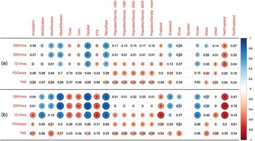
As expected, the correlations become stronger if we limit the analysis to high-quality data (DQ1 basins). In particular, significant correlations can be seen between unit streamflow quantiles Q₉₅ and Q₅₀ and annual rainfall and number of rainy days. Lower positive correlations can also be observed between Q₉₅ and Q₅₀ and maximum and mean catchment elevation, and fractions of total basin area characterized by grassland, bare soil, forest and water. The positive correlation found between Q₉₅ (low-flow index) and forested area is somewhat surprising. Empirical evidence in Brown et al. (2005), for instance, shows lower surface water availability during low-flow periods for catchments with fully developed forested areas, due to deeper root zones characterizing forests and tree plantations relative to field and crops, and associated higher evapotranspiration. However, the relation between basin forest cover and streamflow is not univocal (see e.g. Calder 1998, Moore and Heilman 2011).

We can also observe a strong inverse correlation between streamflow quantiles and mean daily maximum and minimum temperature, annual potential evapotranspiration and fraction of fertilized cropland, which are all expected due to the inverse correlation between runoff production and potential evapotranspiration. Significant but weaker inverse correlations were found between unit streamflow percentiles and cropland. The 1st percentile of unit daily streamflows (Q₁/Area, representing high flow) shows a weak negative correlation with population density (years 1980, 1990, 2000, 2005 and mean value), which is more unexpected. A possible explanation could be the positive correlation between population density and catchment area (large cities are usually found in the lower parts of the rivers), combined with the well-known negative correlation between catchment size and unit flood associated with a low exceedance probability (see e.g. regional envelope curve of flood flows: Castellarin et al. 2005, Castellarin 2007), which is also found in the Danube region.

Concerning the selected descriptors of FDC shape (i.e. slope and TND, total negative deviation, defined in Section 4.1, Equation (2) – the smaller the value the flatter the curve in both cases), significant positive correlations were found with mean daily maximum and minimum temperature and annual potential evapotranspiration, while negative correlations were found with the fraction of water and urbanized area. All positive correlations listed above are to be expected: usually higher temperature and evapotranspiration correspond to more arid climates, where river basin water storage is reduced, causing steeper FDCs; the larger the presence of inland water bodies (e.g. lakes) the larger the natural capability to retard and dampen flood peaks, the flatter the curve. The negative correlation between urbanized area and FDC slope or TND could be analogous to what was observed between high-flow regime and population density; that is, the larger the catchment, the larger the percentage of urbanized areas (big cities and large urbanized area tend to cluster in floodplains, see e.g. Di Baldassarre et al. 2013), the flatter the FDC, due to the increased capability of the catchment to store water (see Castellarin et al. 2013).

There are some additional statistically significant dependencies, which are particularly pronounced if we limit our attention to DQ1 data (Fig. 2(b)). For instance, the analysis points out a significant positive correlation between all unit streamflow percentiles (i.e. Q₁/Area; Q₅₀/Area and Q₉₅/Area) and minimum catchment elevation; it also highlights an inverse correlation between Q₁/Area and population density, and a significant inverse correlation between FDC slope and TND and maximum catchment elevation, population density and fractions of grassland, shrub and water. This is a sensible result as flatter flow–duration curves are associated with higher capability of the catchment to temporarily store water volumes; and this capability generally increases with increasing elevation (winter snowpack), presence of water bodies, or size of the catchment.

3.2 Multi-regression models

We used the above correlation analysis as a basis to identify log-linear multi-regression models for predicting a given dependent variable (i.e. a streamflow index) using catchment descriptors. This was done by applying a stepwise regression analysis (see Draper and Smith 1981, Weisberg 1985) using the R-function lm in R (R Core Team 2016, see also Chambers 1992). We excluded multi-regression models associated with an adjusted R-squared, . To enable a direct comparison to be made with the results reported in Section 4 (i.e. geostatistical interpolation), the accuracy of these models was assessed also in terms of Nash-Sutcliffe efficiency computed for log-transformed (LNSE) and natural (NSE) streamflow percentiles.

3.3 Results and discussion

We were only able to derive acceptable (i.e. ) regression models for streamflow indices Q₅₀ (median discharge), Q₁ (1st percentile) and Q₉₅ (95th percentile), using DQ1 class gauges only. The details of all models are shown in Table 2.

Table 2. Effective multi-regression models (i.e. adjusted R-squared, ) identified for the DQ1 class gauges in the Danube region.

No.	Model		LNSE (NSE)	Scatter plot
1		0.73	0.74 (0.62)
2		0.80	0.80 (0.76)
3		0.66	0.66 (0.57)

The multi-regression model analysis highlights the following aspects:

• it is not possible to identify effective (i.e. ) multi-regression models for all streamflow indices of interest in the Danube region;

• high- and low-flow percentiles (i.e. Q₁ and Q₉₅, respectively) are more difficult to predict than indices of typical streamflow conditions (i.e. Q₅₀);

• including lower quality streamflow data (DQ2 basins) has a negative impact on model performance;

• multi-regression models are characterized by rather limited accuracy despite significant correlations between predictands and some of the predictors; and

• indices of the FDC shape (i.e. FDC slope and TND) cannot be effectively regressed against any of the available catchment descriptors (predictors).

In other words, multi-regression models are not capable of accurately representing streamflow quantiles across all durations (from high-flow to low-flow quantiles) and study area (i.e. high- and low-quality gauges, DQ1+DQ2). Moreover, the unsupervised stepwise regression procedure used in the analysis does not select any catchment descriptor (i.e. predictor) associated with anthropogenic pressure or human presence in the catchment as an explanatory variable in any of the models.

This makes rather evident that resorting to macroscale multi-regression models is not a viable approach for predicting the streamflow regime in ungauged basins located in the Danube region. For this reason, we interpolated the empirical FDCs over the stream network of the Danube basin using the geostatistical method recently proposed by Pugliese et al. (2014, 2016), outlined briefly in the next section.

4 Top-kriging interpolation of flow–duration curves

4.1 Description of the geostatistical interpolation procedure

Topological kriging (or top-kriging) is a geostatistical tool for predicting streamflow indices at ungauged river cross-sections as linear combinations of the empirical information collected at neighbouring gauging stations by taking the stream-network topology into account (Skøien et al. 2006). Top-kriging can be described briefly as a block-kriging with variable support area, in which the support area coincides with a watershed of a given river cross-section; further details on the method can be found in Skøien et al. (2006, 2014).

The scientific literature illustrates successful applications of top-kriging for predicting a wide spectrum of streamflow indices and variables: low flows (see e.g. Castiglioni et al. 2011, Laaha et al. 2014); high flows and floods (Merz et al. 2008, Archfield et al. 2013); stream temperature (Laaha et al. 2013); habitat suitability indices (Ceola and Pugliese 2014); and daily streamflow series (Skøien and Blöschl 2007, de Lavenne et al. 2016, Farmer 2016).

Pugliese et al. (2014, 2016) proposed a method for using top-kriging to predict continuous FDCs at ungauged locations, as opposed to regional regression approaches, which model streamflow quantiles independently of each other. They use an “index-flow” strategy (see e.g. Castellarin et al. 2004) and standardize the empirical FDC at location , , where indicates the duration, for some reference value , to yield a dimensionless FDC:

(1)

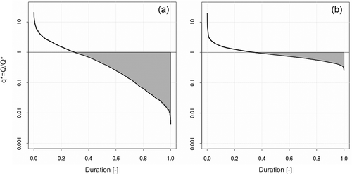
The term can be a given streamflow statistic, such as the long-term average of the daily streamflow series. Then, Pugliese et al. (2014) define an overall index that effectively and objectively summarizes empirical FDCs, differently from FDC slope which is subjectively defined. They name this index total negative deviation (TND), and it is derived by integrating the area between the lower limb of the FDC and the reference streamflow value (see definition sketch in Fig. 3).

Figure 3. Schematic representation of the total negative deviation (TND, shaded area) for two flow–duration curves (FDCs): (a) a steep FDC (fast responding catchment) and (b) a flat FDC (slow responding catchment).

Empirical TND values result from:

(2)

where represents the ith empirical dimensionless quantile standardized for the selected reference value , Δ_i is half of the frequency interval between the (i + 1)th and (i – 1)th quantiles and the summation involves only the m standardized quantiles ≤1. The range of the summation, m, in Equation (2) is set according to the minimum sample length in the regional sample. Having calculated empirical TND values, Pugliese et al. (2014, 2016) proposed using them within top-kriging as a regionalized variable to develop site-specific weighting schemes. The same weights derived through the solution of the linear kriging system for TND are then used for a batch prediction of the continuous, dimensionless FDC for the ungauged site, x₀:

(3)

where , for j = 1, …, n, are the weights resulting from the kriging interpolation of TNDs for the n neighbouring gauged catchments; is the dimensionless, empirical FDC at the donor site x_j, and is the predicted dimensionless FDC. It is worth highlighting that the computation of the kriging weights depends on n, the number of neighbouring sites on which to base the spatial interpolation.

Once a reliable model (e.g. a regional regression model, or kriging model) for predicting at the ungauged site has been set up for the study region, the prediction of the dimensional FDC, , can be obtained as:

(4)

where is the prediction of at ungauged location , and has the same meaning as in Equation (3). For the sake of brevity, this prediction method is referred to as total negative deviation top-kriging (TNDTK). Additional details can be found in Pugliese et al. (2014).

4.2 Implementation of TNDTK to the Danube region

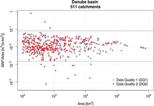
We applied the procedure presented above to the entire Danube region. All analyses were carried out by applying the R-package rtop (Skøien et al. 2014). We selected the mean annual flow (MAF) as the reference streamflow value for standardizing empirical FDCs across the study region. The MAF values are available from the database as long-term average daily discharges. Concerning DQ1 basins located in the Danube region, the minimum value, 25th percentile, median, mean value, 75th percentile and maximum value of empirical MAF are equal to 0.640, 5.90, 28.7, 527, 184 and 6380 m³/s, respectively. Figure 4 illustrates the values of MAF standardized by catchment area as a function of basin area for the study region. Based on values illustrated in Figure 4 and some preliminary TNDTK runs, we regarded as highly discordant all values of MAF/Area outside the interval 0.0015–0.08 m³ s⁻¹ km⁻². All basins with empirical MAF/Area values falling outside this interval were therefore excluded from further analyses. We can observe that all but one of the 14 discarded basins are associated with low-quality (DQ2) streamgauges, which further highlights the low reliability of these outlying values.

Figure 4. Unit mean annual flow as a function of basin area for the Danube region and interval identifying extremely discordant sites (0.08–0.0015 m³ s⁻¹ km⁻²; dashed lines); shape and colour of dots indicate data quality: high (DQ1 - blue open circles) and low (DQ2 - red solid dots).

Therefore, as the Danube region includes a large number of low-quality measurement points (i.e. DQ2 streamgauges, see Fig. 1), we decided to perform all analyses twice, first by focusing only on high-quality data (i.e. DQ1 measuring points, or 137 catchments) and then by considering low- and high-quality data combined (i.e. DQ1+DQ2 measuring points, or 497 catchments). The results of both analyses are reported in the figures in double-panel layouts.

Top-kriging has been applied by fitting the sample variogram of the empirical TND values with a five-parameter fractal–exponential model (for details, see Skøien et al. 2006) through a modified version of weighted least squares regression (WLS; Cressie 1993; for details, see also the neutral WLS method in rtop, Skøien et al. 2014). The fitted variogram model was then used to evaluate the kriging weights for all ungauged sub-basins, based on the n closest neighbouring gauges. Standardized FDCs were then predicted at locations of interest through Equation (3). After a preliminary sensitivity analysis, we set n = 6 in line with previous studies, suggesting to limit the size of the kriging neighbourhood when interpolating streamflow indices, and standardized FDCs in particular (see Pugliese et al. 2014, 2016). The prediction of dimensional FDCs at locations of interest via Equation (4) requires prediction of the local MAF value, which we achieved via a traditional application of top-kriging that uses the same settings listed above (i.e. a modified exponential variogram fitted via WLS regression, neighbourhood size n = 6).

4.3 Cross-validation procedures

We assessed the accuracy of TNDTK predictions in ungauged sites by means of three different validation strategies, which also enabled us to better understand the dependence of the prediction performance on the spatial density of the empirical data. In particular, in order to quantitatively test the reliability and robustness of (a) top-kriging for predicting MAF values, and (b) TNDTK for predicting FDCs in ungauged basins, we performed three leave-p-out cross validation procedures (LPOCVs), in which p coincides with: one site (LPOCV-1), one-third of the sites (LPOCV-⅓) and one-half of the sites (LPOCV-½). All three resampling procedures simulate ungauged conditions at each and every site belonging to the network of N measuring points. In particular, LPOCV-1 drops, in turn, one site at a time and performs the prediction of the streamflow indices of interest in that very site on the basis of the remaining N – 1 measuring points; LPOCV-⅓ (or LPOCV-½) randomly subdivides the N gauged sites into three (or two) subsets and predicts the streamflow indices of interest in all sites belonging to one subset on the basis of the data available at the remaining ⅔N (or ½N) gauging sites. LPOCV-1, LPOCV-⅓ and LPOCV-½ are applied for both DQ1 and DQ1+DQ2 subsets. Finally, we combined LPOCV predictions of MAF (i.e.) and dimensionless FDCs by using Equation (4) to obtain cross-validation predictions of dimensional FDCs at each gauging site in the Danube region. Concerning the prediction of MAF, we quantified the regional accuracy in terms of regional Nash-Sutcliffe efficiency between empirical and predicted log-transformed (LNSE) and natural (NSE) MAF values; concerning the prediction of dimensionless and dimensional FDCs we computed LNSE and NSE values either globally (i.e. assessing overall LNSE and NSE values across all sites and durations, or across all sites but duration-wise) and locally (i.e. at each gauge on the basis of the 15 interpolated streamflow quantiles). Note that the comparison between LNSE and NSE values is important for better understanding the efficiencies of TNDTK for low flows (LNSE) and high flows (NSE).

4.4 Results and discussion

Figures 5, 6 and 7 present, in a similar fashion, the results obtained relative to MAF, dimensionless FDCs and dimensional FDCs (dimensionless and dimensional curves are described through 15 streamflow quantiles). Scatter diagrams distinguish between DQ1 and DQ1+DQ2 subsets and report empirical values vs predictions for the three different resampling strategies used in the study.

Figure 5. Top-kriging interpolation of mean annual flow (MAF) values in cross-validation: empirical (x-axes) vs predicted (y-axes) MAF and Nash-Sutcliffe efficiency for log-transformed (LNSE) and natural (NSE) streamflows. See Section 4.4.2 for the three different resampling strategies used in cross-validation: LPOCV-1 (a, d), LPOCV-⅓ (b, e) and LPOCV-½ (c, f). The LPOCV-1 cross-validated predictions of MAF for the six DQ1 gauges associated with the worst prediction of dimensional FDCs are highlighted (solid dots, red).

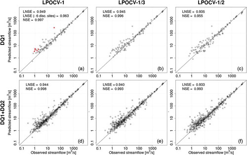
Figure 6. Top-kriging interpolation of standardized flow–duration curves (each empirical curve is standardized by local mean annual flow) in cross-validation: empirical (x-axes) vs predicted (y-axes) dimensionless streamflow quantiles and overall Nash-Sutcliffe efficiency for log-transformed (LNSE) and natural (NSE) streamflows. See Figure 5 caption for further explanation.

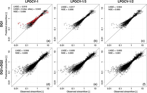
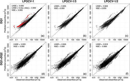
Figure 7. Top-kriging interpolation of dimensional flow–duration curves in cross-validation: empirical (x-axes) vs predicted (y-axes) dimensionless streamflow quantiles and overall Nash-Sutcliffe efficiency for log-transformed (LNSE) and natural (NSE) streamflows. See Figure 5 caption for further explanation.

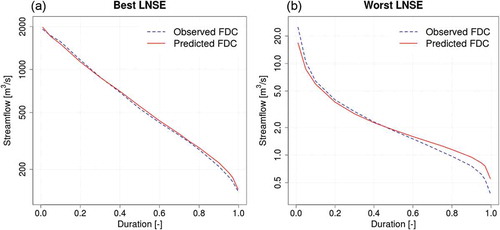
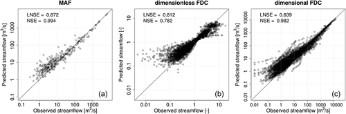
Concerning cross-validated predictions of dimensional FDCs, Figure 8 reports the distributions of local LNSE and NSE values for both DQ1 and DQ1+DQ2 subsets and all resampling strategies, while Figure 9 illustrates LNSE values computed across all DQ1 (or DQ1+DQ2) sites as a function of duration and resampling strategy. Figure 10 shows the comparison between observed and interpolated FDCs for the two gauges having the best and the worst performances in terms of LNSE values for DQ1 – LPOCV-1.

Figure 8. Cross-validation of predicted dimensional FDCs: box-plots of LNSE (red, left box in each box-plot pair) and NSE (blue, right box in each box-plot pair) values computed for all (a) DQ1 and (b) DQ1+DQ2 measurement points for three different resampling strategies used in the study (see Section 4.4.2). Each box shows 25th, 50th (i.e. median) and 75th percentiles; whiskers indicate the most extreme data points that are no more than 1.5 times the inter-quartile range (difference between 75th and 25th percentiles) from the box; outlying values are indicated as circles.

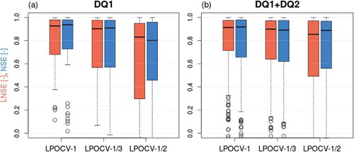
Figure 9. Cross-validation of predicted dimensional FDCs: LNSE values computed across all (a) DQ1 and (b) DQ1+DQ2 measurement points as a function of duration; different curves refer to the three different resampling strategies (see Section 4.4.2).

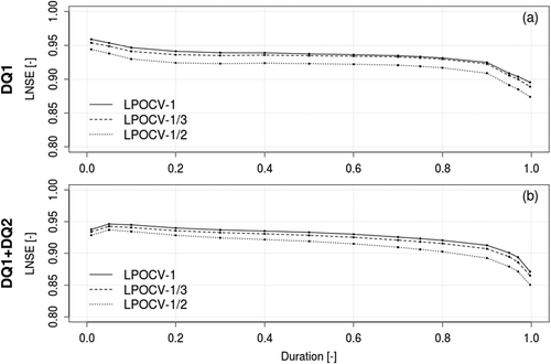
Figure 10. Observed and predicted dimensional FDCs for the two catchments having (a) the best and (b) the worst performance in terms of LNSE in LPOCV-1 for DQ1 measurement points.

The FDCs are of paramount importance for many water-resources management applications (see e.g. Vogel and Fennessey 1995, Yaeger et al. 2012), and therefore the accuracy of interpolated FDCs needs to be properly assessed.

4.4.1 Viability of geostatistical prediction of FDCs over large geographical regions

Figures 5–9 illustrate an overall good agreement between empirical indices of streamflow regimes and their predictions for all three resampling strategies used in cross-validation. In particular, the scatter diagrams between empirical and predicted MAF values in Figure 5 highlight a very good agreement between observed and predicted values, with the majority of points falling in the vicinity of the one-to-one line; as a result, LNSE and NSE values are rather high both for high-quality data (DQ1) and high- and low-quality data (DQ1+DQ2). The overall prediction performance appears almost independent of the resampling strategy, and the detriment of cross-validation predictions remains limited when moving from LPOCV-1 to leave-one-third-out LPOCV-⅓, or to LPOCV-½. It is worth stressing here that the three cross-validation procedures base all predictions only on 136, 68 and 45 measurement points if we consider the DQ1 subset, and a significantly larger number of streamgauges (i.e. 496, 248 and 165) when the DQ1+DQ2 subset is considered. As top-kriging is a geostatistical procedure, its prediction performance should increase with the density of the gauging network. This effect is visible when looking at the LNSEs and NSEs obtained for a single data subset, where LNSE and NSE values slightly decrease for DQ1 (or DQ1+DQ2) when moving from LPOCV-1 to LPOCV-⅓, and LPOCV-½. Yet the same consideration does not hold across datasets, that is, when comparing the results of the same resampling strategy for DQ1 and DQ1+DQ2. The higher number of streamgauges included in the DQ1+DQ2 subset does not result in better MAF prediction due to the lower quality of the streamflow data collected at the additional measuring points.

Figure 6 illustrates the performance of TNDTK for predicting dimensionless FDCs. These scatter plots show an excellent agreement between predictions and empirical data. Overall LNSE and NSE values are well above 0.8 for both subsets and all three resampling strategies. As for the results for MAF predictions, changing the resampling strategy shows a very limited impact on predicted dimensionless FDCs. Including additional streamflow data of lower quality (i.e. DQ2 basins) does not have any significant effect on predicted MAF values and dimensionless FDCs, and therefore the empirical streamflow regime is captured equally well by DQ1 and DQ2 subsets.

Figure 7 shows the relationship between empirical and predicted FDCs in a similar fashion to Figure 6. The cross-validation exercise shows outstanding performance, with overall LNSE and NSE values above 0.9, and the detriment of prediction performance associated with the reduction of gauging network density is, again, very limited. In fact, the scatter plots of Figure 7 show that the overall LNSE values might be significantly impacted by a very limited number of dimensionless FDCs that are poorly predicted. To further discuss this point, LPOCV-1 panels in Figures 5, 6 and 7 highlight (in red) the predictions of MAF, dimensionless and dimensional FDCs obtained for six DQ1 gauges associated with very poor prediction of dimensional FDCs (i.e. the six predicted FDCs are associated with the lowest at-site LNSE values). Closer inspection reveals that these six gauging points are all located in areas where the station density is high, and therefore the low performance should not be attributed to the lack of hydrological information. Figure 5 reveals that poor predictions in terms of dimensional FDCs are mainly associated with poor prediction of MAF, and that five out of six catchments are associated with low or very low empirical values of MAF. In fact, five out of six discordant sites are headwater catchments, for which top-kriging has been already shown to be less effective than for medium to large catchments (see e.g. Castiglioni et al. 2011, Laaha et al. 2014), and whose mean annual flow is likely to be altered by e.g. manmade diversions. The same consideration (i.e. significantly altered streamflow regime) may apply also to larger catchments.

Aside from a small number of peculiar sites, Figures 5, 6 and 7 show a generalized excellent agreement between empirical and predicted streamflow indices and flow–duration curves.

Figure 8 details the local prediction performances through a box-plot representation of the distributions of at-site LNSEs and NSEs between empirical and predicted dimensional FDCs (LNSE and NSE values are computed on the basis of 15 streamflow quantiles; box-plots are truncated at LNSE = 0 and NSE = 0, respectively). It can be seen that, for both DQ1 and DQ1+DQ2 datasets and all three resampling strategies, more than 50% of the predictions are associated with at-site LNSE and NSE values that are above 0.8; in almost all cases 75% of predicted FDCs correspond to LNSE and NSE values in excess of 0.5 (the one exception is for LNSEs in LPOCV-½ for the DQ1 dataset). Figure 8 also shows that there are outlying sites with very low, and sometimes negative, LNSE and NSE values; in particular, negative LNSE (NSE) values are obtained in a number of cases varying from a minimum of 10.9% (12.3%) to a maximum of 16.3% (16.1%) of sites, corresponding to DQ1+DQ2-LPOCV-⅓ (DQ1+DQ2-LPOCV-1) and DQ1-LPOCV-½ (DQ1-LPOCV-⅓), respectively. All these cases are associated with poor predictions of MAF (see also Fig. 5). The box-plots of Figure 8 clearly illustrate the decrease in prediction performance associated with the three considered resampling procedures (and the corresponding reduction of gauging network resolution), which is more evident if results are analysed on an at-site basis relative to the overall performance illustrated in Figure 7.

Finally, the LNSE values computed by comparing duration-wise predicted and empirical streamflow quantiles across all sites for the 15 durations considered in the study (Fig. 9) indicate very good performance in all cases, slightly decreasing for increasing durations but generally well above 0.9 and above 0.85 for all durations and both subsets DQ1+DQ2 and DQ1. The results are similar in terms of NSE values, but are not reported here for the sake of conciseness. Figure 9 confirms the limited impact of reducing the gauging network density through the different resampling strategies; it indicates a high robustness of TNDTK and shows a limited dependence of prediction performance on duration. A slightly worse performance can be noted in the low-flow section of the curves, which was expected. The TNDTK approach features a homogeneous prediction accuracy across all durations, different from conventional quantile regression techniques (see e.g. Blöschl et al. 2013, Castellarin et al. 2013), whose application to the study area resulted in significantly lower efficiencies (see Table 2: LNSEs for 95th, 50th and 1st percentiles for DQ1 class gauges).

It is worth emphasising that the overall LNSE and NSE values are 0.923 and 0.930, respectively, for 137 interpolated FDCs, which were predicted in cross-validation on the basis of 45 measuring points (i.e. less than one gauge per 17 500 km² in the study area), which proves the effectiveness of TNDTK for interpolation of FDCs over large regions (Pugliese et al. 2016).

Figures 5–8 do not show significant differences between efficiencies computed in terms of LNSE or NSE, meaning that TNDTK performances for high and low flows are equivalent. In particular, discharge values reported on y-axes in Figure 10 allow us to confirm that TNDTK performs best for larger catchments, while performance becomes lower for smaller catchments, especially headwater ones (see e.g. Castiglioni et al. 2011, Laaha et al. 2014). In both cases (best and worst LNSE), comparison between the lower tails of observed and predicted FDCs confirms that TNDTK tends to overestimate low flows (see Pugliese et al. 2016).

4.4.2 Indicators of the reliability of interpolated FDCs over large areas

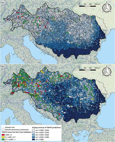
Given the similarity between results in terms of LNSE and NSE, we decided to present the assessment of the reliability of interpolated FDCs by referring to LNSE values only. The maps in Figure 11 highlight the LPOCV-1 for the gauged elementary sub-catchments with an at-site efficiency of cross-validated FDCs (LNSE) lower than 0, between 0 and 0.7, or higher than 0.7. As expected, we can observe that the best performances are typically obtained for nested catchments, large and very large Danube sub-catchments and nodes where station density is higher, while lower performances are associated with headwater catchments located in low-station-density areas.

Figure 11. Prediction variance and local cross-validation LNSE for Danube region elementary catchments: local LNSE values obtained in cross-validation (LPOCV-1 sampling strategy, see Section 4.4.2) at (a) 137 DQ1 streamgauges and (b) 497 DQ1+DQ2 streamgauges are colour-coded; kriging variance is also illustrated.

It would be extremely useful if statements on the expected accuracy were attached to all interpolated FDCs; unfortunately, LNSE values for cross-validated flow–duration curves are available only for gauged elementary catchments (see Fig. 11). A possible measure of prediction uncertainty is the kriging variance (i.e. estimate of the interpolation error), which can be derived for any kriging interpolation scheme and, as such, is an output of each top-kriging application. This statistic is a combination of model uncertainty and configuration of observation locations; so that lower kriging variances are expected for large prediction catchments that are surrounded by several streamgauges, whereas higher variances are expected for prediction nodes located in data-scarce sub-areas and in upstream catchments.

Figure 12 illustrates standardized prediction variances (y-axis) resulting from top-kriging interpolation of empirical TND values as a function of LNSE values of cross-validated FDCs (LPOCV-1 cross-validation, x-axis). Standardization of kriging variances was performed by dividing each value by 0.073, which is the maximum kriging variance computed for the study region and refers to the DQ1+DQ2 dataset. Figure 12 also reports the rolling mean for a subset of 30 catchments.

Figure 12. Standardized kriging variance for TNDTK interpolation procedure as a function of LNSE for (a) DQ1 and (b) DQ1+DQ2 subsets. LNSE values smaller than 0.7 are omitted. Dashed (red) lines represent the rolling mean computed with a rolling window of 30 catchments.

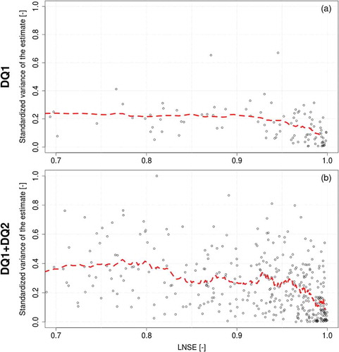
Figure 12 confirms that higher LNSE values are associated with lower kriging variances; the relationship is clearer for the DQ1+DQ2 subset due to the larger sample size, but it is visible also for DQ1. Also, despite the larger number of gauges, Figure 12 clearly shows that the DQ1+DQ2 subset is associated with higher kriging variances relative to DQ1, which is yet another indication of the higher uncertainty and noise of the streamflow information coming from DQ2 streamgauges.

Therefore, kriging variance can be used as a proxy for uncertainty of predicted FDCs. Kriging variance is graphically illustrated in Figure 11 for each ungauged elementary catchment belonging to the Danube region using a colour scale (the darker the colour blue, the higher the variance). It is evident that, in both cases, prediction variance tends to be lower where station density is higher. Comparison between the two maps points out that integrating the gauging network with DQ2 streamgauges may enable one locally to reduce the prediction variance (see e.g. the northeastern portion of the Danube region). Nevertheless, a weighted average of the kriging variance that weights the information proportionally to the size of the considered elementary catchment is equal to 0.042 for the DQ1 subset and to 0.060 for the DQ1+DQ2 subset, and therefore significantly larger for the latter subset. This is consistent with what is reported in Figure 11, which shows that kriging variance for DQ1+DQ2 is significantly larger than for DQ1 in the central portion of the Danube region. Therefore, adding catchments with less accurate streamflow data (DQ2 subset, see Fig. 1) negatively impacts the capability of the geostatistical interpolation procedure to represent the streamflow regime in the central portion of the study region.

This is effectively illustrated in Figure 13, which refers to 360 DQ2 catchments and shows scatter plots of empirical vs geostatistically predicted MAF values (top-kriging), together with dimensional and dimensionless FDCs (TNDTK procedure). These geostatistical predictions are based entirely on the data collected at 137 DQ1 measuring points. As illustrated in Figure 13, the overall performance is analogous to performances illustrated in Figures 5, 6 and 7. The slight decrease in terms of prediction accuracy relative to DQ1+DQ2-LPOCV-½ (i.e. panel (f) in Figs. 5, 6 and 7) is to be expected, and results on the one hand from the reduction of the available empirical data on which interpolation is based (e.g. the ratio between measuring and prediction points is equal to 137/360 = 0.38 in this case, while it is 1 for DQ1+DQ2-LPOCV-½), and on the other hand from the poorer quality of streamflow data collected at DQ2 measuring points, which has been highlighted above.

Figure 13. Top-kriging interpolation in cross-validation, empirical (x-axes) vs predicted (y-axes): (a) mean annual flow (MAF), (b) dimensionless flow–duration curves (FDCs), (c) dimensional FDCs. Predictions refer to 360 DQ2 catchments and are based on observations collected at 137 DQ1 measuring points.

On the basis of these considerations, we decided to use the DQ1 subset to predict FDCs over the whole study region (i.e. 4381 prediction nodes), and we used the kriging variance as an indicator of prediction uncertainty.

5 Conclusions

While streamflow indices are significantly correlated to catchment characteristics within the Danube region, their prediction using multi-regression models may not be satisfactory. A much improved regionalization of empirical flow–duration curves has been obtained for more than 4000 sub-basins in the Danube river basin by using the total negative deviation top-kriging method (TNDTK; see Pugliese et al. 2014, 2016), which was shown to be an effective and accurate interpolation technique across the entire study region. Although the spatial density of the streamgauging network affects the estimation variance of interpolation, it has been proven that the regionalization becomes more accurate when low-quality measurements are discarded. The maps of streamflow quantiles presented herein may be useful for the evaluation of water resources availability at ungauged locations, and as a benchmark for the development of hydrological macroscale models.

Acknowledgements

The data used for this analysis were compiled by DG JRC of the European Commission from the archives of the International Commission for the Protection of the Danube River (ICPDR) and the Global Runoff Data Centre (GRDC). Both institutions are gratefully acknowledged for providing the data. The work is part of DG JRC’s Danube Water Nexus flagship cluster of activities in support of the European Union Strategy for the Danube region (EUSDR) and funded by Service Contract no. C392658.X0-JRC – European Commission. The data layers of interpolated FDC quantiles are accessible through the Danube Reference Spatial Data Infrastructure (DRSDI: http://drdsi.jrc.ec.europa.eu/). The analyses presented in the study use algorithms and tools developed within the European Commission FP7 funded research project SWITCH-ON (Sharing Water-related Information to Tackle Changes in the Hydrosphere – for Operational Needs, grant agreement no. 603587). The study is also part of the research activities carried out by the working group: Anthropogenic and Climatic Controls on WateR AvailabilitY (ACCuRAcY) of Panta Rhei – Everything Flows, Change in Hydrology and Society (IAHS Scientific Decade 2013–2022). All figures included in the study were produced by the use of free and open-source software (i.e. Quantum GIS Geographic Information System - Open Source Geospatial Foundation Project, http://qgis.osgeo.org, and the R Project for Statistical Computing, https://www.R-project.org/).

Disclosure statement

No potential conflict of interest was reported by the authors.

Additional information

Funding

This work was supported by the Joint Research Centre [C392658.X0-JRC].

References

- Archfield, S.A., et al., 2013. Topological and canonical kriging for design flood prediction in ungauged catchments: an improvement over a traditional regional regression approach? Hydrology and Earth System Sciences, 17, 1575–1588. doi:10.5194/hess-17-1575-2013
- Bierkens, M.F.P., et al., 2015. Hyper-resolution global hydrological modelling: what is next? Hydrological Processes, 29, 310–320. doi:10.1002/hyp.10391
- Blöschl, G., et al., 2013. Runoff prediction in ungauged basins: synthesis across processes, places and scales. New York, NY: Cambridge University Press, 465. ISBN-13: 9781107028180.
- Brown, A.E., et al., 2005. A review of paired catchment studies for determining changes in water yield resulting from alterations in vegetation. Journal of Hydrology, 310, 28–61. doi:10.1016/j.jhydrol.2004.12.010
- Calder, I.R., 1998. Water use by forests, limits and controls. Tree Physiology, 18 (8–9), 625–631. doi:10.1093/treephys/18.8-9.625
- Castellarin, A., 2007. Probabilistic envelope curves for design flood estimation at ungauged sites. Water Resources Research, 43, W04406. doi:10.1029/2005WR004384
- Castellarin, A., 2014. Regional prediction of flow-duration curves using a three-dimensional kriging. Journal of Hydrology, 513, 179–191. doi: 10.1016/j.jhydrol.2014.03.050
- Castellarin, A., et al., 2013. Prediction of flow duration curves in ungauged basins. In: G. Blöschl, et al., eds. Runoff prediction in ungauged basins: synthesis across processes, places and scales. Cambridge, UK: Cambridge University Press.
- Castellarin, A., Vogel, R.M., and Brath, A., 2004. A stochastic index flow model of flow duration curves. Water Resources Research, 40, W03104. doi:10.1029/2003WR002524
- Castellarin, A., Vogel, R.M., and Matalas, N.C., 2005. Probabilistic behavior of a regional envelope curve. Water Resources Research, 41, W06018. doi:10.1029/2004WR003042
- Castiglioni, S., et al., 2011. Smooth regional estimation of low-flow indices: physiographical space based interpolation and top-kriging. Hydrology and Earth System Sciences, 15, 715–727. doi:10.5194/hess-15-715-2011
- Ceola, S. and Pugliese, A., 2014. Regional prediction of basin-scale brown trout habitat suitability. In: A. Castellarin, et al., eds. Evolving water resources systems: understanding, predicting and managing water–society interactions. Vol. 364. Wallingford, UK: International Association of Hydrological Sciences, IAHS Publ, 26–31.
- Chambers, J.M., 1992. Linear models. Chapter 4. In: J.M. Chambers and T.J. Hastie, eds. Statistical models. Pacific Grove, CA: S. Wadsworth & Brooks/Cole.
- Collischonn, W., et al., 2007. The MGB-IPH model for large-scale rainfall–runoff modelling. Hydrological Sciences Journal, 52, 878–895. doi:10.1623/hysj.52.5.878
- Cressie, N.A.C., 1993. Statistics for spatial data, Series in probability and mathematical statistics: applied probability and statistics. Chichester, UK: J. Wiley.
- de Lavenne, A., et al., 2016. Transferring measured discharge time series: large-scale comparison of top-kriging to geomorphology-based inverse modeling. Water Resources Research, 52, 7. doi:10.1002/2016WR018716
- de Paiva, R.C.D., et al., 2013. Large-scale hydrologic and hydrodynamic modeling of the Amazon River basin. Water Resources Research, 49, 1226–1243. doi:10.1002/wrcr.20067
- de Roo, A., et al., 2012. A multi-criteria optimisation of scenarios for the protection of water resources in Europe: support to the EU blueprint to safeguard Europe’s waters. Publications office of the European Union, JRC75919. doi:10.2788/55540
- Di Baldassarre, G., et al., 2013. Towards understanding the dynamic behaviour of floodplains as human–water systems. Hydrology and Earth System Sciences, 17 (8), 3235–3244. doi:10.5194/hess-17-3235-2013
- Donnelly, C., Andersson, J.C.M., and Arheimer, B., 2016. Using flow signatures and catchment similarities to evaluate the E-HYPE multi-basin model across Europe. Hydrological Sciences Journal, 61, 255–273. doi:10.1080/02626667.2015.1027710
- Draper, N.R. and Smith, H., 1981. Applied regression analysis. 2nd ed. Hoboken, NJ: John Wiley & Sons.
- Falter, D., et al., 2016. Continuous, large-scale simulation model for flood risk assessments: proof-of-concept. Journal of Flood Risk Management, 9, 3–21. doi:10.1111/jfr3.12105
- Farmer, W.H., 2016. Ordinary kriging as a tool to estimate historical daily streamflow records. Hydrology and Earth System Sciences, 20, 2721–2735. doi:10.5194/hess-20-2721-2016
- Laaha, G., et al., 2013. Spatial prediction of stream temperatures using top-kriging with an external drift. Environmental Modeling & Assessment, 18 (6), 671–683. doi:10.1007/s10666-013-9373-3
- Laaha, G., Skøien, J.O., and Blöschl, G., 2014. Spatial prediction on river networks: comparison of top-kriging with regional regression. Hydrological Processes, 28 (2), 315–324. doi:10.1002/hyp.9578
- Merz, R., Blöschl, G., and Humer, G., 2008. National flood discharge mapping in Austria. Natural Hazards, 46 (1), 53–72. doi:10.1007/s11069-007-9181-7
- Moore, G.W., and Heilman, J.L., 2011. Proposed principles governing how vegetation changes affect transpiration. Ecohydrology, 4 (3), 351–358. doi:10.1002/eco.232
- Parajka, J., et al., 2015. The role of station density for predicting daily runoff by top-kriging interpolation in Austria. Journal of Hydrology and Hydromechanics, 63. doi:10.1515/johh-2015-0024
- Pechlivanidis, I.G. and Arheimer, B., 2015. Large-scale hydrological modelling by using modified PUB recommendations: the India-HYPE case. Hydrology and Earth System Sciences, 19, 4559–4579. doi:10.5194/hess-19-4559-2015
- Pugliese, A., et al., 2016. Regional flow duration curves: geostatistical techniques versus multivariate regression. Advances in Water Resources, 96, 11–22. doi:10.1016/j.advwatres.2016.06.008
- Pugliese, A., Castellarin, A., and Brath, A., 2014. Geostatistical prediction of flow–duration curves in an index-flow framework. Hydrology and Earth System Sciences, 18, 3801–3816. doi:10.5194/hess-18-3801-2014
- R Core Team, 2016. R: a language and environment for statistical computing. Vienna, Austria: R Foundation for Statistical Computing. Available from: https://www.R-project.org/
- Sampson, C.C., et al., 2015. A high-resolution global flood hazard model. Water Resources Research, 51, 7358–7381. doi:10.1002/2015WR016954
- Skøien, J.O., et al., 2014. rtop: an R package for interpolation of data with a variable spatial support, with an example from river networks. Computers and Geosciences, 67, 180–190. doi:10.1016/j.cageo.2014.02.009
- Skøien, J.O. and Blöschl, G., 2007. Spatiotemporal topological kriging of runoff time series. Water Resources Research, 43 (9), W09419. doi:10.1029/2006WR005760
- Skøien, J.O., Merz, R., and Blöschl, G., 2006. Top-kriging – geostatistics on stream networks. Hydrology and Earth System Sciences, 10, 277–287. doi:10.5194/hess-10-277-2006
- Vogel, R.M. and Fennessey, N.M., 1995. Flow duration curves II: a review of applications in water resources planning. JAWRA Journal of the American Water Resources Association, 31, 1029–1039. doi:10.1111/j.1752-1688.1995.tb03419.x
- Wei, T. and Viliam, S., 2016. corrplot: visualization of a correlation matrix. R-package version 0.77. Available from: https://CRAN.R-project.org/package=corrplot
- Weisberg, S., 1985. Applied linear regression. 2nd ed. New York: John Wiley & Sons.
- Westerberg, I.K., et al., 2016. Uncertainty in hydrological signatures for gauged and ungauged catchments. Water Resources Research, 52, 1847–1865. doi:10.1002/2015WR017635
- Yaeger, M., et al., 2012. Exploring the physical controls of regional patterns of flow duration curves – part 4: a synthesis of empirical analysis, process modeling and catchment classification. Hydrology and Earth System Sciences, 16, 4483–4498. doi:10.5194/hess-16-4483-2012