How the performance of hydrological models relates to credibility of projections under climate change

ABSTRACT

Two approaches can be distinguished in studies of climate change impacts on water resources when accounting for issues related to impact model performance: (1) using a multi-model ensemble disregarding model performance, and (2) using models after their evaluation and considering model performance. We discuss the implications of both approaches in terms of credibility of simulated hydrological indicators for climate change adaptation. For that, we discuss and confirm the hypothesis that a good performance of hydrological models in the historical period increases confidence in projected impacts under climate change, and decreases uncertainty of projections related to hydrological models. Based on this, we find the second approach more trustworthy and recommend using it for impact assessment, especially if results are intended to support adaptation strategies. Guidelines for evaluation of global- and basin-scale models in the historical period, as well as criteria for model rejection from an ensemble as an outlier, are also suggested.

KEYWORDS:

• hydrological model performance
• climate change impact
• uncertainty of projections
• calibration and validation
• rejecting model as outlier
• guidelines for model evaluation

Editor R. Woods Associate editor G. Di Baldassarre

1 Introduction

Climate impact research is currently evolving from impact studies to development of adaptation strategies and provision of climate services. In the water sector, these services are now starting to provide detailed, high spatial resolution information on projected climate change impacts in the future for specific water-related indicators, to be directly applied in adaptation measures (Kaspersen et al. 2012). Projections of climate impacts are always connected with uncertainties, whereas stakeholders typically prefer to use crisp numbers, ignoring spreads of projections. Therefore, different approaches are being developed to create awareness of uncertainty, and guide users for robust decision making under uncertainty. The modellers and data providers at present face a large responsibility to achieve confidence in the model results for climate change adaptation that is undertaken locally.

The projection of future water resources is usually done by following a complex modelling chain, often starting with assumptions regarding future radiative forcing (e.g. representative concentration pathways, RCPs) and climate projections by general circulation models (GCMs) to regional climate models (RCMs), or statistical downscaling methods, to bias correction of climate data, and finally through hydrological impact models to obtaining final results (see details in the reviews by Olsson et al., 2016, Krysanova et al. 2016). Following this chain, it is becoming more common to use not only ensembles of climate projections, but also sets of impact models, i.e. ensembles of hydrological models (Haddeland et al. 2014, Roudier et al. 2016, Donnelly et al. 2017, Vetter et al. 2017).

Different types of hydrological models (HMs) are used for impact assessment; they can be global- (gHM) or regional/basin-scale (rHM), simplified conceptual or process-based, high resolution, semi-distributed or spatially lumped. The numerical models were originally developed for different purposes, such as flood forecasting (e.g. HBV, see Bergström 1976), process understanding (e.g. SHE, see Refsgaard et al. 2010), predictions in ungauged basins (e.g. TOPMODEL, see Beven and Kirby 1979), large-scale water resource estimates (e.g. WaterGAP, see Döll et al. 2003), agricultural water management issues (SWAT, see Arnold et al. 1993) or surface-water quality management (e.g. HYPE; see Lindström et al. 2010). The scale of a model may be not fixed, as there are models originally developed for the basin scale that are applied also for the continental and global scales (such as HYPE, SWAT, LISFLOOD), and models developed for the global scale that are applied for large river basins (e.g. VIC and WaterGAP3). The various model concepts are often assigned with different approaches to evaluate model performance, and sometimes with different attitudes to the importance of model calibration and validation.

From the beginning of the 1990s, the catchment modelling community developed sophisticated optimization and uncertainty algorithms (e.g. Beven and Binley 1992, Duan et al. 1993, Vrugt et al. 2003), which are frequently applied to judge reliability of rHMs for specific purposes and sites. Thus, rHMs in climate impact studies are generally calibrated and validated specifically to the site of interest. On the contrary, most gHMs are usually applied for impact studies with a global parameterization, which compromises the quality of local performance for assumed good performance globally, i.e. using a priori estimates of individual process parameters (e.g. see Vörösmarty et al. 2000), or after calibration only for selected large catchments (e.g. Döll et al. 2003, Widén-Nilsson et al. 2007), or combinations of these approaches (e.g. Nijssen et al. 2001). It is impossible to achieve good performance at all locations and basins using these methods, so generally a rHM will provide better performance than a gHM at the location for which a rHM has been tuned. However, more rigorous calibration procedures are now starting to be developed for gHMs (e.g. Müller Schmied et al. 2014), and continental-scale HMs (e.g. Donnelly et al. 2016, Hundecha et al. 2016) including multiple objective calibration, also for variables other than discharge (e.g. Viney et al. 2009, Andersson et al. 2017).

Recently, the outputs from global- and regional-scale hydrological models were compared in the Inter-Sectoral Impact Models Intercomparison Project (ISI-MIP) (Gosling et al. 2017, Hattermann et al. 2017) for their performance and impacts in terms of mean seasonal dynamics of river flow, mean annual discharge and high/low flows.

In general, two different approaches can be distinguished in climate change impact studies when applying impact models and accounting for issues related to model performance:

Approach 1: Using a multi-model ensemble disregarding performance. This approach is widely used for climate impact assessment by global- and continental-scale modelling studies (Dankers et al. 2014, Gosling et al. 2017) and follows the state of the art for ensembles of GCM and RCM projections used by the IPCC (IPCC 2014). It is assumed that every participating model has equal opportunity (sometimes called “one model, one vote”), and some modellers even claim that the multi-model application is not “a beauty contest” as an argument supporting this approach. For example, Christensen et al. (2010) suggested that an unweighted multi-model mean is the best approach for RCM projections, because no single model is best for all variables, seasons and regions (see also Kjellström et al. 2010). This has also been assessed for gHMs (Gudmundsson et al. 2012a, 2012b), based on a study of the performance of nine gHMs (including land surface schemes, LSS), suggesting that a central tendency of a multi-model ensemble (mean or median) should be presented as the output in climate change impact studies, despite (and because of) the large variations in performance of individual models.

Approach 2: Using models considering their performance. This approach is also widely applied for impact assessment. Several authors (e.g. Prudhomme et al. 2011, Roudier et al. 2016) have underlined the importance of model performance and suggested that the impact model ensemble should be adjusted according to the performance of the HMs in reproducing the indicators to be projected (e.g. river discharge). This could be done by removing the outliers or poorly performing models, or weighting the individual models’ results based on their results in the reference period. Hydrological impact assessment often involves the output of one or more indicators for which the performance under historical climate conditions can be evaluated specifically. This approach follows the tradition of catchment modellers to choose between parameter values during calibration, and only accept the best model performance. Nowadays, it is often extended to using not one but several parameter sets that demonstrated a good performance, enabling also uncertainty assessment (Beven and Binley 1992, 2014, Seibert 1997, Beven 2009, Yang et al. 2014).

There are both advantages and disadvantages in each of these two approaches when applied for climate change impact assessment. A comparison of these two approaches allows us to compare also uncertainties related to impact models and connect them with the model performance.

For instance, the first approach may be the only feasible one on short notice for global- and continental-scale assessments (e.g. IPCC) that are used to raise awareness about potential changes and hotspots in future water resources, and to allow impact assessments also in data poor regions. However, the global-scale models may not provide an accurate description of the hydrological system at a given location, river basin or region for the period of available observations (e.g. Dankers et al. 2014, Hattermann et al. 2017). Besides, this approach has some obvious weaknesses, because e.g. a removal of one single outlier model that consistently overestimates or underestimates runoff percentiles could shift the ensemble mean far from the level corresponding to the situation when all models are used (Gudmundsson et al. 2012a, Fig. 4), and how should this be interpreted? Also, the ensemble approach requires large modelling resources, and is only meaningful if there is consensus among the model groups about the model protocol and simulation experiments.

The second approach, on the other hand, is herein considered more reliable at the catchment scale and could give confidence to decision makers to implement adaptation measures. If simulations for the historical period closely represent observations, the projections based on such models are more easily accepted by model users (e.g. Borsuk et al. 2001). This approach involving calibration and validation procedures is also more time consuming and computationally demanding, especially when applied for large domains using complex process-based models.

However, it can be argued that equifinality in the parameter choices (Beven 2006) and adjustment of parameters to present climate might not give robust parameter values that are valid also for a changed climate. Still, checking the model(s) performance, allowing for equifinality (e.g. using the GLUE methodology: see Beven and Binley 1992) and involving an ensemble of parameter sets will be more robust than using a single “optimum” parameter set, and this should still be a part of best practice (e.g. see Cameron et al. 2000). Nevertheless, this does not mean that the resulting ensemble of parameter sets will provide good simulations under future climate conditions, for a number of reasons. This calls for calibration and validation procedures that at least ensure that the model’s ability to respond to the longer scales of variability in today’s climate is as good as possible.

Traditionally, gHMs are applied for climate impact assessments at global and continental scales with a coarse spatial resolution (e.g. 0.5 degree), while rHMs are applied in impact studies mostly for one or several river basins (Bergström et al. 2001, Andréassian et al. 2004, Aich et al. 2014, Vetter et al. 2015) or at the national or large river-basin-scale with a high spatial resolution (Huang et al. 2010, 2013a, 2013b, Arheimer et al. 2012, Hattermann et al. 2014, 2015, Arheimer and Lindström 2015). Recently, rHMs have started to be applied also at the continental scale (Archfield et al. 2015, Donnelly et al. 2016), or for multiple large river basins worldwide (ISI-MIP project, see Krysanova and Hattermann 2017, Krysanova et al. 2017) based on model evaluation done in advance (Huang et al. 2017). The gHMs are moving towards a finer resolution of up to ~1 km (Bierkens et al. 2015). Thus, the two impact-modelling communities are approaching each other’s spatial domains and should also benefit from sharing their best practices.

In this paper, we argue that both approaches for assessing climate impacts are useful in the right context, but it is important to be aware of the differences, and the uncertainties related to model performance should be always mentioned. In particular, we intend to discuss implications of the second approach recognizing the importance of model performance, and whether it helps to achieve more reliability in water indicators for climate change adaptation. To do this, we intend to prove or reject the hypothesis that good performance of hydrological models in the historical period increases confidence in projected impacts under climate change, and decreases uncertainty of projections related to hydrological models. This will be done mainly based on literature review and analysis of some modelling results, and guided by the following partial questions:

1. When does a model become a poor tool for describing the behaviour of a basin and thus should be excluded from an ensemble as an outlier?

2. What is the influence of model performance in the control period on the outcome of impact assessment? Namely, does a good performance of HMs increase their credibility for impact assessment and decrease uncertainty of projections related to hydrological models, or not?

3. How should model evaluation be done in the context of climate impact assessment?

2 Performance of global and regional HMs and cross-scale evaluation

First, we would like to stress that, in our opinion, it is the model’s performance at the location of interest in the period with observations that is important, and not whether or not the model was calibrated and validated to that location. Sometimes a non-calibrated model may perform well enough, and the calibration may lead to problems related to over-tuning.

Usually we assume that a model performs well when it is evaluated for several indicators, and a number of evaluation criteria, describing certain hydrological signature(s) (e.g. river discharge, or percentile Q₁₀), are in the good or satisfactory performance categories vs observations. The judgment of a “good performance category” depends on the considered hydrological signature, its temporal resolution, spatial scale, evaluation criteria used and quality of observational data (Kauffeldt et al. 2013, Beven and Smith 2015). Guidelines for model evaluation have been formulated in several papers (e.g. Moriasi et al. 2007, Tuppad et al. 2011, Ritter and Muñoz-Carpena 2013). Here we briefly discuss performance of global models, regional models and a cross-scale evaluation of both model types based on recent literature.

2.1 Performance of global hydrological models

The performance of gHMs used in impact studies tends to vary with location and catchment scale, which means that, while at some points it may be considered good, in many cases it can be very poor. A number of studies evaluated the performance of gHMs by comparing different simulated aspects of runoff. Table 1 provides an exemplary overview of evaluation of eight global hydrological models and one continental-scale model applied in the manner of gHMs, not pretending to give a full picture or include all existing gHMs. Please note that nearly all of these are maintained models, meaning that they are continuously updated and improved and that the values in this table simply reflect the state of the model at the time of the publication cited. For a more complete list of gHMs and their main features, see Bierkens (2015), Bierkens et al. (2015), Sood and Smakhtin (2015) and Kauffeldt et al. (2016). A comprehensive summary of previous global and continental model evaluation protocols can be found in Beck et al. (2017).

Table 1. Overview of evaluation for a suite of global- and continental-scale (E-HYPE) models of different types based on river discharge. Examples are chosen from respective single-model evaluation studies. Note: many of the global- and continental-scale HMs are managed models that are constantly updated and improved. Values reflect model performance found in recent publications. NSE: Nash-Sutcliffe efficiency; PBIAS: percent bias; RMSE: root mean square error; r: Pearson correlation coefficient; Q: river discharge; P: precipitation; CV: coefficient of variation.

Model name, scale of application	Number of basins, range of catchment sizes	Evaluation approach: aspects of runoff checked and criteria of fit applied	Results in terms of criteria	Visual evaluation/comparison	Large discrepancies found for	References
HD (MPI-HM), global	6 basins of Baltic Sea, Arctic Ocean, Godavari, Mississippi, Ganges/Brahmaputra, Yangtze	None	None	Comparison of long-term mean monthly dynamics simulated with two climate re-analysis datasets	Overestimation for Mississippi with both climate datasets	Hagemann and Dümenil Gates (2001)
VIC, global	26 large river basins, 117 900 to 4.62 × 10^6 km^2	Individual evaluation of monthly flow with RMSE and PBIAS	After calibration: │PBIAS│< 20 in 18 cases; │RMSE│< 50 in 12 cases	Comparison of mean monthly hydrographs and mean annual runoff for selected basins	Overestimation in hot and arid basins (e.g. Senegal)	Nijssen et al. (2001)
Mac-PDM, global	50/42 basins with 10–30 years of data, 44 320 to 4.64 × 10^6 km^2	Aggregated evaluation of average annual runoff for all 50 catchments with r	r = 0.93 (aggregated results for all catchments)	Comparison of long-term mean monthly values (runoff regime) for 42 catchments	Overestimation in dry basins (e.g. Murray, Niger and Red)	Gosling and Arnell (2011)
WaterGAP 2.2, global	1319 basins with 4–30 years of data, 9000 to 1.2 × 10^6 km^2	Individual evaluation of time series of monthly river discharge with NSE	NSE > 0.5 in 53.5% of all stations	Comparison of discharge seasonality for 12 selected basins; map of NSE values in three classes	Poorer performance in arid climate zone: NSE < 0.5 in 72% of the catchments	Müller Schmied et al. (2014)
PCR-GLOBWB, global	2219/1938/26 basins with ≥10 years of data, 2312 to 3.68 × 10^6 km^2	Individual evaluation for 1938 (26) stations using relative deviation in average runoff and correlation coefficient (r) of monthly and annual discharges (slope and coefficient of determination, R^2)	Seasonality: for 75% of the gauged area, r > 0.75; inter-annual variability: for 60% of the gauged area, r > 0.75	Comparison of long-term mean monthly values (discharge seasonality) for 26 stations	Large overestimation in dry basins: Niger, Orange, Nile and Murray. Under-estimation in Arctic/sub-Arctic basins.	Van Beek et al. (2011)
LPJmL, global	213 basins with ≥5 years of data in 1979–1999, 8542 km^2 to 4.62 × 10^6 km^2	Individual evaluation of average annual discharge comparing ranges of uncertainty of simulated Q driven by seven P datasets with observed Q	Observed Q for 95 (+23) basins within ranges of uncertainty of simulated Q (+ difference <10%)	Differences in % on a map	Overestimation in African basins, Mississippi, Murray, Parana	Biemans et al. (2009)
H08, global	32 basins >200 000 km^2 with streamflow records for >60 months in 1986–1995	Individual evaluation of mean annual discharge using normalized bias (NBIAS), difference in timing of peak Q PEAK, and correlation coefficient of variation in Q	NBIAS ≤ ±0.2 for 14 stations, PEAK ≤ 1 for 16 stations, r ≥ 0.8 for 13 stations	Normalized monthly simulated and observed streamflows are compared	Low performance for Sao Francisco, Parana, St. Lawrence, Don, Lena. Five rivers in arid zone not evaluated.	Hanasaki et al. (2008)
MATSIRO-GW, global	20 large river basins with observed records for max. 15 years (1985–1999)	Individual evaluation of monthly Q time series using NSE and relative bias	NSE > 0.5 in 11 of 20 basins, relative bias < 20% in 11 basins	Comparison of long-term mean monthly values (discharge seasonality) for 20 basins	Weak performance in dry rivers and underestimation of discharge peak in high-latitude rivers	Koirala et al. (2014)
E-HYPE, continental	Calibration: 115 small, representative gauged basins without lakes, validation: 538 independent gauged basins of varying size	NSE; PBIAS; percentiles Q5, Q95, Q50; CV of daily flow (Hundecha et al. 2016) Flow signatures (Donnelly et al. 2016)	Median NSE = 0.53, median PBIAS = 1.3% over 538 validation stations	Employed to some extent in the calibration process (to daily discharge hydrographs)	Weaker performance on the Iberian peninsula and in regulated rivers, underestimation of Q in Fennoscandia	Hundecha et al. (2016), Donnelly et al. (2016)

As one can see from Table 1, a highly heterogeneous number of basins, criteria, validation periods, data products (climate forcing, discharge data) and evaluation criteria have been used in different studies. The thresholds of fit are not always explicitly defined and documented for all studied basins, and the performance varies greatly among the basins and studies. Satisfactory results in terms of long-term average annual or monthly runoff are usually found for approximately 50% of all gauge stations considered, and the rest show poor comparison with observations (Table 1). The most comprehensive evaluation of monthly discharge for more than 1000 gauge stations globally was done with the PCR-GLOBWB and WaterGAP2.2 models (Van Beek et al. 2011, Müller Schmied et al. 2014), and in both cases the quality of climate forcing data was discussed in relation to the evaluation results.

Poor performance: systematic overestimation of runoff in arid and semi-arid areas, and systematic underestimation of discharge in high-latitude river basins, can be noted for most examples presented in Table 1 for gHMs. This indicates systematic biases across models in representing specific processes such as snowmelt in high latitudes and evaporation in drylands (see e.g. Gerten et al. 2004), but can also be attributed partly to the climate forcing datasets and their uncertainties (see e.g. paper by Biemans et al. (2009), who compared seven global precipitation datasets in relation to the performance of one gHM). Thus, we can conclude that a comprehensive, systematic evaluation for all models (also for variables other than discharge), using the same set of evaluation metrics and observational databases, is needed.

Often, gHM performance is evaluated in several large-scale catchments for river discharge only, yet impact results are delivered for multiple hydrological indicators on maps at all scales from far upstream (one grid cell) to far downstream (many grid cells accumulated), as well as for a number of internal model variables such as evapotranspiration, soil moisture and runoff. It is also becoming common to use gHMs not only for studying changes in mean seasonal dynamics, but also to investigate changes in extreme runoff characteristics, such as magnitude and frequency of high/low flows, floods, hydrological droughts and water scarcity under climate change scenarios (Dankers et al. 2014, Prudhomme et al. 2014, Schewe et al. 2014, Arnell and Gosling 2016, Gosling et al. 2017). This has mostly been done without any checking of model performance for the indicators of extremes in advance in these and other global-scale studies. As a result, huge projection uncertainties and even contradicting projections based on gHMs appear in the literature (Kundzewicz et al. 2017), and stakeholders may be confused.

However, there do exist several studies that evaluated performance in more detail, e.g. for a set of three to nine uncalibrated gHMs in Europe using a database of discharge observations in very small, pristine catchments (mostly sub-grid scale) which were assumed to represent grid-scale runoff. The evaluations included spatially aggregated runoff percentiles (Gudmundsson et al. 2012a), seasonality of the runoff at grid and spatially aggregated scales (Gudmundsson et al. 2012b), and indices describing extremes of runoff (Prudhomme et al. 2011). This was a valuable contribution to understanding how these sorts of models perform at the grid to sub-catchment scale. These studies showed that there are large variations in local model outputs, large variations in model performance when aggregating outputs over larger areas, biases in both mean and variability of simulated runoff, and increasing biases at the extreme ends of the flow duration curve. It was shown that in many cases individual models perform extremely poorly. However, while Gudmundsson et al. (2012a) suggested that each model was a hypothesis to be tested, conclusions as to whether any of these “model hypotheses” should be rejected were not made, and instead the multi-model ensemble was suggested to be used for climate impact analysis.

Recently, Beck et al. (2016) presented a new globally regionalized model evaluated in over 1787 catchments ranging in size from 10 to 10 000 km², and, more importantly, presented a comparison of the performance of nine state-of-the-art gHMs using common metrics. They showed that the median performance of many of these models across the range of evaluated catchments is rather poor. For example, median Nash and Sutcliffe efficiencies (NSE) were well below zero, i.e. adequacy of the used gHMs to described processes is worse than knowing the mean flow (i.e. the observed mean is a better predictor than the models). Notably, the new model presented with regionalized calibration outperformed even the ensemble mean of the other nine gHMs. Here, it seems appropriate to quote the Nobel laureate in chemistry, Sir C. N. Hinshelwood (1971, p. 22, 1966/67, p. 24): “It is sometimes claimed that the results even if rough will be useful statistically. There can be no more dangerous doctrine than that based upon the idea that a large number of wrong or meaningless guesses will somehow average out to something with a meaning.”

2.2 Performance of regional-scale models

In contrast to gHMs, performance of regional models is always tested in advance for the region/river basin under study, most often using daily or monthly discharge dynamics, but less often for other variables: high and low percentiles of discharge, evapotranspiration, return periods of floods and low flow. Table 2 presents an overview of evaluation of regional hydrological models for large regions, which was done relative to the indicators of interest of impact assessment.

Table 2. Overview of evaluation of regional-scale models applied for several large river basins or regions with calibration/validation for multiple gauges. Note: the regional-scale HMs are constantly updated and improved; the values in this table reflect model performance found in recent publications. NSE: Nash-Sutcliffe efficiency; r: Pearson correlation coefficient; PBIAS: percent bias; LNSE: logNSE; NSEiq: NSE on inverse flows; KGE: modified Kling-Gupta efficiency; VE: volumetric efficiency; Δσ: percent bias in standard deviation; ΔFMS, ΔFHV and ΔFLV: percent bias in flow duration curve mid-segment slope, high-segment volume, and low-segment volume, respectively; ΔFlood and ΔLF: percent bias in the 10- and 30-year flood levels and low-flow levels, respectively.

Model name	Region(s) or river basins, number of gauges for evaluation	Criteria of fit used for evaluation	Results in terms of criteria of fit	Visual evaluation/comparison	Large discrepancies or weaker results found	References
S-HYPE	Sweden and/or Baltic Sea catchment	NSE, PBIAS and visual fit for daily discharge, simulated trends 1961–2010 also compared.	Median absolute PBIAS = 8%, median NSE approx. 0.7 (157 stations)	Visual fits as additional criteria for daily discharge, and internal model variables	Median NSE for unregulated/regulated basins = 0.75/0.55	Strömqvist et al. (2012), Arheimer and Lindström (2015)
SWIM	Germany: 5 large river basins: Elbe, Weser, Ems, Rhine, Upper Danube with 38 gauges for evaluation	NSE, LNSE, PBIAS	NSE > 0.6 in 89/84%, PBIAS < ±15 in100/90%, LNSE < 0.6 in 89/84% in calib./valid. periods	Graphs in papers	Catchments with substantial water management	Huang et al. (2010), 2013a, 2013b)
ECOMAG	Lena (2490 000 km^2), Amur (1855 000 km^2), MacKenzie (1805 000 km^2), Northern Dvina (357 000 km^2), Pechora (322 000 km^2) with 41 gauges for evaluation	NSE, PBIAS for daily discharges	NSE > 0.70 in all gauges, PBIAS < ±15 in all gauges, NSE > 0.85 in all river outlets, PBIAS < ±10 in all river outlets	Graphs in papers	Weaker performance for low flow	Motovilov et al. (2013), Gelfan et al. (2015, 2017)
SWAT	Vistula (194 000 km^2) and Odra (119 000 km^2) basins, with 106 gauges for evaluation	KGE and its three components with daily time step	KGE > 0.5 in 88/81%, KGE > 0.6 in 78/55%, PBIAS < ±15 in 77/65% of gauges in calib./valid. periods	Mapped evaluation results for KGE but no clear spatial patterns revealed	Weaker performance for smaller catchments	Piniewski et al. (2016)
HBV	ISI-MIP: 8 basins: Rhine, Tagus, Upper Niger, Blue Nile, Upper Yellow, Upper Yangtze, Upper Mississippi, Upper Amazon – 67 000 to 991 000 km^2; evaluation at outlet	NSE, NSEiq, KGE, VE, PBIAS, Δσ, r, ΔFMS, ΔFHV, ΔFLV, ΔFlood, ΔLF	NSE > 0.7 in 8/8, PBIAS < ±15 in 7/8, FHV < ±25 in 7/7, FLV < ±25 in 2/7	Graphs in Huang et al. (2016)	Weaker evaluation results for low flow	Huang et al. (2017), Vetter et al. (2017)
MGB-IPH	South American basins (Amazon, Rio Grande, Upper Paraguay, etc.)	NSE, LNSE, PBIAS	Amazon: NSE > 0.6 in 70% of 69 gauges, PBIAS < 15% in 75% of gauges; Rio-Grande: NSE > 0.85, PBIAS < 7%, LNSE > 0.87 in 100% of gauges	Graphs in papers	Weaker performance for smaller catchments	Nóbrega et al. (2011), Bravo et al. (2012), Paiva et al. (2013)

As we can see, good evaluation results, in terms of two to three criteria of fit, have been achieved for most of the gauges in all studies, whereas a poorer performance has been stated for a few gauges, mostly in catchments with intensive water management, low runoff coefficient or for low flow. Going to the multi-basin and national-scale applications with the models developed for the catchment scale and assuring their good performance is possible in principle, though not easy (Strömqvist et al. 2012).

However, the applied evaluation/validation techniques used for all HMs usually do not assess how a model might perform in a different climate (e.g. checking specifically for dry or wet periods, depending on the expected future climate), although it is important for the following impact studies. Validation of a model in different climates can be done by (a) using a differential split-sample, or DSS, test, as suggested by Klemeš (1986) and Refsgaard et al. (2013a), (b) testing the model under different combinations of the calibration/evaluation periods including the period of changes in hydrological regime (e.g. Choi and Beven 2007, Coron et al. 2012, Gelfan et al. 2015), (c) testing the model’s ability to reproduce inter-annual variability (Greuell et al. 2015), or (d) a combination of these methods to give more credibility to the fact that the model can perform well in a changing climate for certain indicators (or should be declined for some indicators). Note that the hierarchical test scheme for model validation developed by Klemeš (1986) distinguishes simulations under stationary and non-stationary conditions as well as for gauged and ungauged basins.

Several recent studies across the globe have addressed these methods. For instance, the study of Choi and Beven (2007) on the multi-period and multi-criteria evaluation of TOPMODEL in a catchment of South Korea has shown that, while the model fitted very well in a classical sense for the whole calibration period, the dry period clusters did not provide parameter sets consistent with other periods. Coron et al. (2012) tested three conceptual rainfall–runoff models over a set of 216 catchments in Australia in contrasting climate conditions using a generalized split-sample test, and showed that validation over a wetter (drier) climate than during calibration led to an overestimation (underestimation) of the mean runoff, whereas the magnitude of the models’ deficiency depended on the catchment considered. In the study of two basins, one characterized by changes in climatic conditions and the second exposed to a drastic land-cover change due to deforestation, Gelfan et al. (2015) showed that it is possible to simulate changes in hydrological regime with acceptable accuracy, retaining the stable model structure and parameter values. Fowler et al. (2016) analysed 86 catchments in Australia and showed that DSS-test can miss potentially useful parameter sets, which could be identified using an approach based on Pareto optimality, suggesting that models may be more capable under changing climatic conditions than previously thought.

Examples of testing a range of catchment models under changing climate and anthropogenic conditions and successful evaluation of their ability to cope with them were provided in a Special Issue of Hydrological Sciences Journal on “Modelling temporally-variable catchments” (Thirel et al. 2015).

2.3 Cross-scale evaluation of both types of models

Recently, hydrological simulations carried out with the help of nine gHMs and nine rHMs for 11 large river basins in all continents were analysed and inter-compared under reference and scenario conditions (Hattermann et al. 2017). The rHMs were calibrated and validated using the re-analysis WATCH forcing data (WFD, Weedon et al. 2011) as input and applying a split-sample approach, whereas the gHMs were not calibrated (with the exception of one). The outputs of five GCMs from CMIP5 (Taylor et al. 2012) were statistically downscaled and used as climate forcing under four RCPs. They were bias-corrected using the WATCH data as reference and applying the method described in Hempel et al. (2013).

However, comparison of the WATCH data against locally available observational climate data in the reference period revealed that some variables did not match the observations in some basins (e.g. global radiation in the Niger, and precipitation in the Upper Amazon). In the case of the Niger, the Hargreaves equation with Tmin and Tmax as input variables was used to calculate global radiation, which led to a significantly improved comparison of the simulated discharge against measurements (Aich et al. 2014). For the Upper Amazon with tropical cloud forests, the cloud water interception was included using the Tropical Rainfall Measuring Mission data (Strauch et al. 2017), also leading to improvement of model performance. Despite these modifications, the conclusions regarding rHMs and gHMs in this study should hold, because rHMs generally give even better results than gHMs outside of controlled experiments, such as in Hattermann et al. (2017), because rHMs often use local forcing data utilizing all available information.

One major result of the inter-comparison for the reference conditions is that the global models often show a considerable bias in mean monthly and annual discharges and sometimes incorrect seasonality, whereas regional models show a much better reproduction of reference conditions. The mean of gHMs performs better than most individual models due to a smoothing effect, but the bias is still quite large.

Hattermann et al. (2017) summarized the model evaluation results for two model ensembles considering only their aggregated outputs: the long-term mean monthly dynamics averaged over each model set. The evaluation was done using two criteria of fit: correlation coefficient (r) between the simulated and observed mean annual cycles of the period 1971–2000 and bias in standard deviation (Δσ). In addition, the d-factor (Abbaspour et al. 2007), which is the ratio of the average distance between the 97.5 and 2.5 percentiles and the standard deviation of the corresponding measured variable, defined as a measure of uncertainty, was applied.

According to the accepted thresholds, high correlation (≥0.9) was found for 10 basins for means of rHMs, but for only four out of 11 basins for means of gHMs; and low bias in standard deviation (<±15%) was found in nine cases for means of rHMs, but only in one case out of 11 for means of gHMs. The values of d-factor below 1 denoting a low uncertainty related to observations were found for nine basins simulated with rHMs, but only for one basin simulated with gHMs. Poor performance was found even for the aggregated gHM outputs: the means of nine global models, whereas the regional models demonstrated good performance in this respect, and also individual rHMs were successfully evaluated for monthly and seasonal dynamics as well as high flows (see Huang et al. 2017). We can conclude that performance varies systematically between the calibrated rHMs and non-calibrated gHMs in favour of the regional models.

2.4 When does a model become a poor hypothesis for the behaviour of the basin?

Based on this overview of the HMs’ performance, one may ask: When does a model become a poor hypothesis for the behaviour of the basin and thus should be excluded from an ensemble as an outlier? Even those who are less interested in calibration or evaluation must accept the need for arguments why a model should still be considered useful. In our opinion, there are at least three well-established statements for judging models (see e.g. discussions in Klemeš 1986, Coron et al. 2011, Refsgaard et al. 2013a, Thirel et al. 2015).

First, we agree that a hydrological model can never be universally validated, yet its performance can be evaluated for situations that imitate the “target” conditions (e.g. impact assessment) of the model application. Second, if the model does not perform well (in accordance with the definition above), it is most likely inadequate in the “target” conditions. Third, the opposite is not always true: a lack of disagreement does not necessarily result in the model applicability for these conditions; however, appropriate evaluation design increases credibility and decreases uncertainty in the model results. According to Klemeš (1986), the adequacy of a hydrological model should be judged only from the point of view of the credibility of its outputs.

Besides, the model performance also depends on the adequacy of the forcing data, which is not always consistent and adequate: e.g. see Kauffeldt et al. (2013), who examined the consistency between input climate data and discharge data; Pechlivanidis and Arheimer (2015), who analysed errors and inconsistencies in global databases in application to India; and the discussion of disinformation in data and its effect on model calibration and evaluation by Beven and Westerberg (2011) and Beven and Smith (2015). There are also useful discussions (Beven 2006, 2012, 2016) about facets of uncertainty and possibilities of rejecting potentially useful models because of poor observational data (false negative error), or accepting poor models just because of poor observational data (false positive error), suggesting that we should take a much closer look at the input data to be used for calibration. Therefore, evaluation of the forcing data should be always done in advance.

The listed statements allow us to argue that a model intended to reproduce, for example, the seasonal runoff regime (or other indicators of interest, e.g. high and low percentiles) should be excluded from an ensemble as an outlier, if:

1. it tends to overestimate/underestimate the long-term average annual runoff (or indicators of extremes) significantly (e.g. by >25%, see Moriasi et al. 2007);

2. it cannot reproduce seasonality sufficiently well, e.g. seasonality of flood generation (this can be tested using coefficient of correlation r and bias in standard deviation with thresholds r < 0.8, bias > 25% as criteria of rejection); or

3. it cannot reproduce historical inter-annual variability (e.g. measured by bias in standard deviation exceeding 25%), or deviate significantly in performance between specified periods or between dry and wet periods in the past.

If evaluation is being done for many stations, NSE < 0.5 could be used as a criterion of rejection (see Roudier et al. 2016). The suggested criteria for seasonality were used in Huang et al. (2017) and Hattermann et al. (2017), but with stronger thresholds than proposed here.

Criteria and thresholds for model evaluation focused on streamflow simulation and considering uncertainty of measured data, which could also be used for specifying ensemble outliers, can be found in the guidelines by Moriasi et al. (2007). Nevertheless, we argue that flexibility and pragmatism should be used in applying these thresholds, as the potential to achieve a certain model performance is dependent on the quantity and quality of data available, the catchment size, anthropogenic impacts, climate conditions and the flow regime. Alternatively, the GLUE limits of acceptability approach suggested and applied for flood frequency estimation in Blazkova and Beven (2009) and for discharge prediction in Liu et al. (2009), which is based on analysis of different sources of uncertainty and accounts for observational errors, can be used.

The ability of a model to maintain consistent performance across varying climatic periods (e.g. in a split-sample approach) is more important than extremely high performance in one period, as the level of performance across multiple periods is more indicative of the model’s potential consistency in a future climate. Therefore, models that deviate significantly in performance among several periods should be rejected. And, of course, overall inaccurate performance should be grounds for model rejection.

Whichever approach is used, we argue that a model should not be used for impact assessment if it could not perform well at the validation or verification stage, i.e. it should not be used for projecting indicators it has shown to be poor in reproducing. Under verification here we mean additional model testing under conditions substantially differing from those used for the calibration and validation. For example, if projection of low flows and droughts is of interest or if it is expected that dry periods will increase in future, the use of models that showed difficulty in reproducing dry periods (e.g. Choi and Beven 2007, Chiew et al. 2014) should be excluded, or, alternatively, an approach to allow for non-stationarity of parameters should be found.

However, in practice there are, on the one hand, studies evaluating performance of state-of-the-art continental- and global-scale models, where large errors are found for non-calibrated models considering different indicators (e.g. see Haddeland et al. 2011, Greuell et al. 2015, Zhang et al. 2016, Beck et al. 2017), and, on the other hand, numerous climate impact studies where these models are applied and projections presented without any form of verification.

To summarize, the following problems related to uncalibrated gHMs can be listed: poor performance in many regions or river basins; high spreads and uncertainty of climate impact projections; projections by multiple gHMs using the same or similar climate input may contradict, i.e. not be robust; zooming in on specific regions is usually not recommended. And the following problems related to calibrated rHMs can be listed: the model evaluation is time consuming and labour intensive, especially for larger regions; the comprehensive split-sample and spatially-distributed approach using several indicators is not always applied; and going to the continental/global scale maintaining comprehensive model evaluation is not easy.

3 Influence of model performance on results of impact assessment

3.1 Influence of model performance on impacts and their credibility

The meaning of credibility can be different (depending on who is judging) – credibility perceived by the scientific community may not coincide with credibility perceived by the stakeholders or users of model results. Sometimes, these two groups have opposing views on this issue. Whereas both approaches 1 and 2 for climate impact assessment defined in the Introduction are being applied by scientists, using their own arguments, for the users of model results probably Approach 2 is more trustworthy (Borsuk et al. 2001).

There are several studies showing that model performance influences results of impact assessment, and two model sets developed for global and regional scales with different performance in the historical period produce different results.

3.1.1 Example 1: continentally and locally calibrated model

Simulated impacts of climate change on the seasonality of discharge in the Kizilirmak River in eastern Turkey (catchment size 6673 km²) are shown in Figure 1 using both a continentally (analogous to a gHM) and a locally (analogous to a rHM) calibrated model using the same model inputs. The E-HYPE v2.1 model was first calibrated/validated as a continental-scale model for 181 gauges across Europe (see Donnelly et al. 2016 and Table 1), and then calibrated locally for this catchment in Turkey (Fig. 2). The local calibration was manual and aimed to maximize NSE, but a large NSE value was only accepted if the relative error (RE, or percent bias) was within 15%. Then the E-HYPE model was forced by five regionally downscaled global climate models for RCP4.5.

Figure 1. Comparison of climate change impacts on the annual cycle of discharge (top) and snow depth (bottom) for (a) a continental-scale and (b) a locally calibrated E-HYPE v2.1 model – Sögutluhan gauge on the Kizilirmak River in eastern Turkey. The outputs are from the E-HYPE model forced with an ensemble of five regionally downscaled GCMs for RCP4.5. Grey shading shows the reference period (1971–2000), and red shading, a future period (2071–2098). The minimum, median and maximum of the ensemble are shown.

Figure 2. Comparison of observed and simulated discharge at Sögutluhan gauge, Turkey, from the large-scale E-HYPE v2.1 model (blue) and using a model extracted from E-HYPE v2.1 and calibrated locally for this catchment (red). Model performance: large-scale: volumetric error = – 68%, NSE = 0.09; calibrated for the catchment: volumetric error = +9.8%, NSE = 0.75.

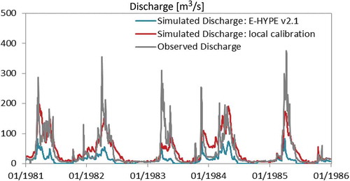
Large differences in model performance, particularly in volumetric errors (–68% vs +9.8%), affect the simulated climate change signal (Fig. 1). In the former model application (Fig. 1(a)), there is no spring flood peak in the future climate, and instead the largest discharges are seen in winter. In the latter model simulation (Fig. 1(b)), the spring flood peak is projected to remain, but decrease in magnitude. This is a significant difference in the projected climate impacts, particularly if a user is primarily interested in flow regime.

The differences in these projections are caused by a smaller snowpack in the continental-scale model, i.e. the mean annual maximum snow depth over 30 years was 140 cm in the calibrated vs 100 cm in the uncalibrated model which has a poor performance, meaning a large underestimation in volume, 68%, at this particular site (Fig. 2). The performance of the continental-scale model is particularly poor at this location; however, this is not unusual when selecting a specific catchment from a large-scale model application. Of course, it can be argued that the locally calibrated model is also uncertain, which is certainly the case. However, it would be misleading to consider the projections of spring flood changes from the continental-scale model equally probable, as the changes are caused by the near depletion of a snowpack that was too small in the reference period. This example falsifies the assumption that all large-scale models are good enough representations of hydrological conditions to be used in specific catchments. We can therefore conclude that the projections of the model calibrated specifically for the catchment are more credible due to better process representation.

3.1.2 Example 2: calibrated and non-calibrated model

In a second example, numerical experiments were carried out with two versions of the ECOMAG regional hydrological model in application to the Lena River basin: (a) with a priori assigned parameters, and (b) with three parameters (controlling snowmelt, evaporation and soil infiltration capacity) adjusted through calibration against long-term daily runoff data in several streamflow gauges. The daily meteorological inputs were assigned using WATCH re-analysis data (Weedon et al., 2011), which demonstrated a good agreement with available meteorological observations.

First, the ability of the GCM-driven model for runoff simulation in the historical period (1971–2005) was tested (Fig. 3(a) and (b)) using climatology data from an ensemble of five GCMs: GFDL-ESM2M, HadGEM2-ES, IPSL-CM5A-LR, MIROC-ESM-CHEM and NorESM1-M, which were bias-corrected in advance against the WATCH re-analysis data. The long-term mean hydrograph (averaged over time and five model runs) simulated by the non-calibrated model (Fig. 3(b)) demonstrates a visible shift of snowmelt flood in comparison with the corresponding hydrograph derived from the calibrated model, and, importantly, in comparison with observations. The main reason is in advancing the snowmelt season by the non-calibrated model from the beginning of June to the middle of May. In addition, the non-calibrated model significantly overestimates runoff in the period from mid-July to mid-November.

Figure 3. Long-term average hydrographs for the Lena basin simulated by (a, c) calibrated and validated and (b, d) not-calibrated ECOMAG model driven by five GCMs in the reference (1971–2005) and end-century (2070–2099) periods. (a, b) Comparison with observed discharge in the reference period, and (c, d) comparison of projections for the end-century (ensemble mean with uncertainty bounds) with ensemble mean in the reference time. cv: calibrated and validated model; nc: not calibrated model; ref: reference period; p3: end-century period.

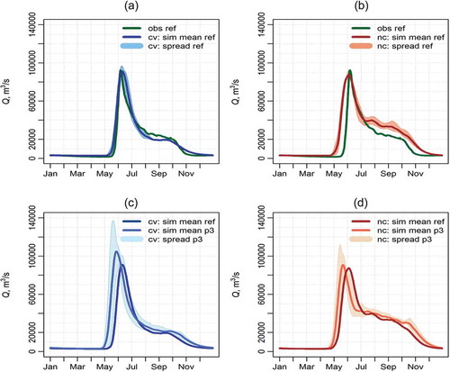
Then, two model versions were used for projecting hydrological response to climate change using the same GCM ensemble and four RCP scenarios for the end-century period (2070–2099). Figure 3(c) and (d) shows different responses from two model versions. The non-calibrated model (Fig. 3(d)) retains tendencies of earlier snowmelt flood and increased summer flow in comparison with the results obtained with the calibrated model, and does not project any visible changes in the long-term mean peak flow discharge compared to the reference (1971–2005) period. At the same time, the calibrated ECOMAG model (Fig. 3(c)) projects an increase in peak flow discharge by more than 15% (ensemble mean) in comparison with the reference period, and a two-week shift of peak flow from mid-June to the end of May. Similar to the previous example, we can conclude that due to better process representation, the projections by the calibrated model in Figure 3(c) are more plausible than those in Figure 3(d).

3.1.3 Example 3: excluding the outlier models

Rejecting the outlier models due to their performance was applied first at the scale of a single model for a single catchment using the limits of acceptability approach, when many sets of sensitive model parameters were tested as potential models of the catchment (Blazkova and Beven 2009). For example, the climate impact study on flood frequency for a catchment in the UK by Cameron et al. (2000) and the flood frequency assessment for a catchment in Czech Republic by Blazkova and Beven (2009) showed the effects of uncertainties in parameterization of hydrological models and in observational data.

There are also examples of multi-impact model studies where models have been selected or omitted from an ensemble based on their performance. For example, the full model ensemble of five HMs from the IMPACT2C project was not included in the paper by Roudier et al. (2016), as some impact models were omitted from the ensemble after validating their performance for extremes. First, a detailed validation of all HMs focusing on average conditions was performed (Greuell et al. 2015), and one of the models showed a large negative bias of 38%, whereas the ability to simulate inter-annual variability did not differ much among the models. After that, the models’ skill in simulating indicators of extremes (magnitudes of 10- and 100-year floods and low flows) was tested, assessing whether the median of an indicator computed based on the 11 bias-corrected climate runs is close to the same indicator computed with observed discharge data for 428 stations (Roudier et al. 2016). For that, the threshold of 0.5 for NSE was used for model rejection, and, finally, an ensemble consisting of three models was selected for floods, and two models for low-flow modelling.

Figure 4 shows an example how excluding improbable models from an ensemble affects the climate change signal and spread. Here we show the simulated impacts in terms of changes in discharge at +2°C (using the method of Vautard et al. 2014 to define climate change at 2°C) for the Kalix River catchment in Sweden using five continental-scale HMs: HYPE, LISFLOOD, LPJml, VIC and WBM and seven climate model projections. After excluding two of the HMs (VIC and LPJml), which were shown to have problems with simulating seasonality (and thus snow processes, Greuell et al. 2015), the median climate change signal increases while the spread of possible responses decreases.

Figure 4. Projected changes in discharge at +2°C for the Kalix River catchment in Sweden using an ensemble of five continental-scale HMs and a reduced ensemble of three HMs which excludes two models that failed to reproduce the seasonality of discharge. The uncertainty ranges are also due to seven driving climate model projections for RCPs 2.6 and 4.5 (see Roudier et al. 2016, Donnelly et al. 2017, for methodology).

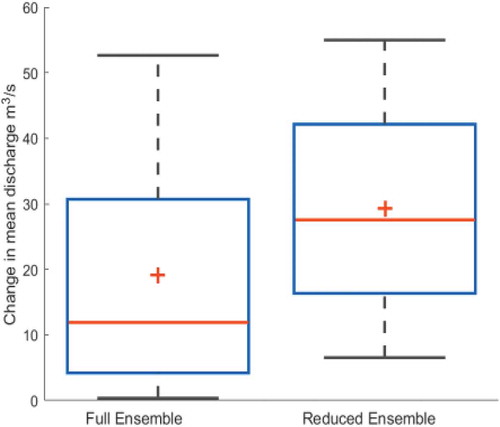
While it is likely that we underestimate the spread in plausible responses with the reduced ensemble, using implausible models to achieve increased spread is simply misleading. In this case, the poor performance of hydrological models could be due to lack of calibration, inappropriate model structure, poor observational data, or deficient description or parameterization of some key processes for the catchments studied. For example, it was later shown that a frozen soil routine was causing unrealistic processes in VIC (Greuell et al. 2015). We do not argue here that three selected models are plausible enough (e.g. due to equifinality and uncertainty in climate input), but we argue that discarding implausible models leads to improving the robustness of results, which may lead to improvement of decision making based on these results.

So, the two HM ensembles in this example show markedly different median discharge changes and uncertainty ranges. We can cautiously conclude that excluding improbable models affects the projected climate impacts and uncertainty ranges, and the projections of the reduced ensemble including models with good performance are more credible. However, more experiments based on larger ensembles of HMs are still required.

3.1.4 Example 4: cross-scale comparison of calibrated rHMs and non-calibrated gHMs in ISI-MIP

A comparison of simulated climate change impacts for gHM and rHM ensembles was done in a study by Hattermann et al. (2017) for 11 large-scale river basins after the evaluation of their performance in the historical period (described in Section 2.3). The comparison of simulated climate change impacts in terms of changes in the long-term average monthly dynamics for gHM and rHM ensemble medians and spreads has shown that:

• the signals of change according to a Wilcoxon test were similar in five out of 11 cases (Rhine, Upper Niger, Ganges, Upper Mississippi and Lena);

• the means and medians were comparable (<50% difference) in two out of 11 cases (Ganges and Lena); and

• the spreads were well comparable (<20% difference) in four out of 11 cases (Lena, Upper Amazon, Upper Yangtze and Upper Yellow).

Two of the 11 basins, the Lena and the Ganges, seem to show the best comparison based on two or three criteria listed above. However, for the Lena, seasonality of discharge simulated by two model ensembles is very different (see Fig. 5), and therefore none of the 11 basins examined in this study could demonstrate similarity based on all three criteria and seasonality patterns.

Figure 5. Evaluation of hydrological model performance in the Lena River basin: long-term average daily discharge driven by WATCH climate data in the reference period 1971–2000 simulated by (a) regional models, rHMs, and (b) global models, gHMs. (c) Simulated climate change impacts modelled by both model types comparing long-term average daily discharge in the scenario period 2070–2099 and reference period. The ranges in (c) are due to five driving GCMs as well global and regional hydrological models.

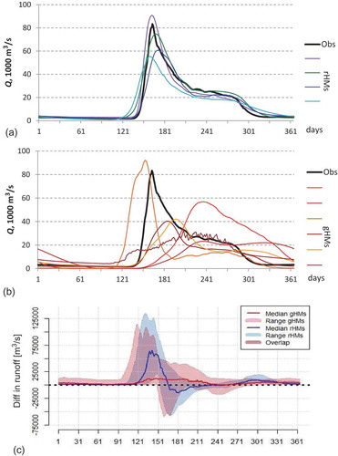
One illustrative example for the Lena River basin stems from that study (Hattermann et al. 2017) and is presented in Figure 5 (with slightly different sets of models). Four regional-scale models (ECOMAG, HYPE, SWIM and VIC), and six global-scale models (DBH, H08, LPJmL, MATSIRO, MPI-HM and PCR-GLOBWB) were used. The gHMs were applied with 0.5° resolution, whereas the three rHMs (ECOMAG, HYPE and SWIM) used much finer spatial disaggregation into sub-basins and hydrotopes, and one (VIC) into 0.5° grids with the sub-grid heterogeneity accounting method. The comparison of model outputs, both visually and statistically, showed good performance of rHMs (Fig. 5(a)), and rather poor performance of most gHMs, with large underestimation and significant delay in flood peaks (Fig. 5(b)).

The better performance of rHMs compared to gHMs is probably due mainly to: (a) better representation of snow accumulation and snowmelt processes in the three of four regional models with finer spatial resolution, which is crucial for flood dynamics in this basin; and (b) the calibration of regional models, which also leads to better representation of snow and runoff processes. According to Gudmundsson et al. (2012b), the low performance of hydrological models in snow-dominated regions is primarily related to the timing of the mean annual cycle, and could be associated with the parameterization of snow dynamics and sub-grid variability of elevation.

In our case (Fig. 5(c)), the medians of simulated changes in discharge at the end-century from two model ensembles are very different and follow the patterns of their performance in the reference period. In other words, the regional models project a substantially increased snowmelt flood in May and June shifted to an earlier period and lower discharge in mid-summer, whereas the gHM ensemble projects a moderate increase in discharge in May–August (Fig. 5(c)).

Therefore, we can conclude that not only does the performance of two model sets differ, but also the results of impact assessment are not comparable. Probably, this is partly due to the fact that the model performance influences the results of the impact study, though it cannot be quantified strictly in this example. The question is, which results are more credible: the ones based on the non-calibrated gHMs with a poor performance, or those of the regional-scale models with better performance? Following Approach 2, we can conclude that the change pattern suggested by regional models is, probably, more trustworthy.

3.1.5 Weighting of impact models

There are also studies where weighting of impact models based on their performance was applied. An early study by Cameron et al. (2000) for assessment of climate impact on flood frequency used likelihood weighting to create uncertainty bounds on future flood frequencies, albeit at that time driven by climate changes from only a single GCM run. The study of Gain et al. (2011) applied weighting of 12 GCMs via hydrological model PCR-GLOBWB; rather than statistically downscaling each of the GCMs based on local meteorological data they attached a weight to each of the GCM-HM simulated outputs, based on similarity of the observed discharge. Recently, Yang et al. (2014) analysed probabilistic climate change projections for the headwaters of the Yellow River, China, with weights assigned to downscaling methods and three hydrological models. The study aimed at quantifying the uncertainties from different sources in simulating extreme flows and constructing reliable scenarios of future extreme flows.

3.2 Influence of model performance on uncertainty of projections

The gHMs applied in ISI-MIP show large ranges in the evaluation period (Hattermann et al. 2017), and, consequently, also give very wide spreads in impacts compared to the regional models in most cases. This paper evaluated the spreads in the long-term average seasonal dynamics of runoff, and found that spreads from gHMs were higher than those from rHMs in 10 basins (of 11), and in three basins the spreads from gHMs were more than doubled as compared to spreads from rHMs (in the Tagus, Upper Niger and Darling). Another study (Gosling et al. 2017) compared relative changes in simulated mean annual runoff and indicators of high and low extreme flows between the two ensembles. Whilst some consistency in the median values between the two ensembles was found in this study, the spreads were generally wider for the gHM ensemble than for the rHM ensemble in most catchments. This leads to the question: Are the models with poor performance misleading the users on the known projection uncertainties?

Also Clark et al. (2016) argue that characterizing uncertainties throughout the modelling process (rather than using an ad hoc “enssemble of opportunity”) is important, followed by reducing uncertainties through developing criteria for excluding poor methods/models, as well as with targeted research aimed at improving modelling capabilities.

The overview of studies described in this section performed with one or several models allows us to respond provisionally to Question 2 (in the absence of further studies dedicated to that very problem and showing the opposite). That is, a good performance of hydrological models in the reference period increases their credibility, both for scientists and for users, regarding the results of impact assessment, and leads to a reduction of uncertainty bounds.

3.3 Main hypothesis: arguments pro and contra

In addition, we try to analyse here some common arguments related to our main hypothesis. The arguments pro and contra the main hypothesis, which are based on numerous literature sources, are listed and commented on in Table 3.

Table 3. Arguments pro and contra (respectively, for and against) the hypothesis that “good performance of hydrological models in the historical period increases confidence of projected impacts under climate change, and decreases uncertainty of projections related to hydrological models”. Comments on arguments P1–P5 and C1–C5 are included in columns 2 and 4. Comments in italics undermine the main hypothesis, and comments in bold (some of them, a kind of “solution”) support the main hypothesis.

Arguments pro	Comments on arguments pro	Arguments contra	Comments on arguments contra (can the contra arguments be weakened, disrupted or “solved”?
P1. Given a good calibration/evaluation procedure that takes into account performance of multiple processes (runoff, evapotranspiration, snow, discharge at multiple sites), there is a higher chance that the relative levels of simulated runoff, evapotranspiration and snow storage are correct, also under changing climate conditions.	However, such a procedure is applied quite rarely.	C1. Good performance under historical conditions is not a guarantee for good performance under different climatic conditions.	Yes, but application of an appropriate calibration/evaluation procedure (as in P1 and P2) may be a remedy.
P2. Validation of a model in different climates, by either (a) subdividing the time series, e.g. as suggested in Refsgaard et al. (2013a) or (b) testing the same parameter set in multiple climates, may augur better for satisfactory model performance in a changing climate.	(a) This procedure is rarely applied. (b) Testing the same model in different basins/climates is often done, but then the model is mostly re-calibrated. This approach should be more extensively tested and promoted.	C2. Poorly designed calibration procedures can compromise the scenario validity of the model (e.g. when calibrated to wet conditions while the future is drier, etc.).	A “good” model should be able to respond to changes in driving climate. For that, the calibration procedure should be appropriately designed (as in P1 and P2).
P3. Poor performance of a model set in a historical period often leads to impacts with uncertain signals of change and large spreads in projections (Hattermann et al. 2017, Gosling et al. 2017).	It is possible that outlying models cause large uncertainties in the ensemble. Hence, a good model performance is important for credible projections.	C3. Traditional split-sample calibration, and using many calibration parameters, may lead to overtuning of a model, which compromises its performance under changed climate (outside of comfort zone) (e.g. Viney et al. 2009) and credibility of projections.	This can be solved, if the calibration/evaluation procedure is appropriately designed (as in P1 and P2).
P4. In the case of Approach 1 (see Introduction) being used: excluding one poor model outlier can change the ensemble mean considerably (Gudmundsson et al. 2012a), hence the ensemble mean is not credible. The same is true for median, though median is usually more robust to outliers.	This is a weakness of Approach 1.	C4. Even a well-calibrated model may be not reliable under significant climate change (Merz et al. 2011), as future climate puts calibrated parameters outside the range in which they were tested.	However, validation of a model in different climates (as in P2) may increase the model reliability.
P5. Model users and stakeholders usually like to see comparison of simulated historical discharge with observations (Borsuk et al. 2001), and tend not to trust results originating from poorly performing models.	Hence, a good model performance is important for acceptance of projections by users.	C5. Modellers should rely on realistic parameter values taken from the literature, and accept model performance as it is, without calibration.	But the realistic parameter values are often indicated as ranges; is a calibration still needed then?

To summarize, all contra arguments in Table 3 suggest that good performance of a hydrological model in today’s climate does not guarantee robust results under different climates. We argue that this can be, in principle, solved by designing frameworks for comprehensive model evaluation that take into account model responses to changing climate, and model responses to several key processes such as runoff, evapotranspiration and snow (as a focus only on streamflow may be too simplistic). Of course, these requirements are quite demanding for the modelling community, and their realization is not straightforward and easy. However, it seems that this is the only way to achieving more robust impact projections and low uncertainty related to hydrological models. In our view, there is a need to agree on a framework for model evaluation within the impact modelling community (see Section 4).

We can conclude that the examples presented in this section and comments to arguments in Table 3 support the main hypothesis of the paper that a good performance of hydrological models in the historical period increases confidence of projected impacts under climate change, and decreases uncertainty of projections related to hydrological models.

However, good performance of a hydrological model in the historical period is just the necessary but not sufficient condition for extrapolating the model’s capabilities to the future. Of course, there are some examples in which such extrapolation would not work; see, for instance, the counter-example in Blazkova and Beven (2009), where parameter conditioning (even within the GLUE context) failed to reproduce the frequency behaviour in a different historical period, and rejection of parameter sets depended on the particular realization of the inputs used.

3.4 Uncertainty of projections and adaptation

Since the model-based projections of climate impact on water resources are often different, for various reasons, adaptation procedures need to be developed that do not rely on a single projection of changes in hydrological variables, but rather are based on ensembles and multi-model probabilistic approaches and use ranges of projected values. Expectations of some water managers to be able to get a crisp value of a needed characteristic of future river flow are futile.

Part of uncertainty is irreducible, and therefore the relevant courses of action may follow the precautionary principle and adaptive management (Di Baldassarre et al. 2011, Kundzewicz et al. 2018). The concepts of precautionary allowances are being envisaged as part of “climate proofing” exercises. “Climate change adjustment factors” have been already introduced in some countries of Europe, where water management specialists are incorporating the potential effects of climate change into specific design guidelines.

The precaution-based adjustments should be taken into account in new plans for flood risk reduction (see Olsson et al. 2016, Kundzewicz et al. 2017). For instance, traditional design values of precipitation or river flow are increased by a safety margin in order to be on the safe (or safer) side. The value of the safety margin may reflect the existing, model-based, river flow projections that may span a large range due to the spread of future climate trajectories, even if the hydrological models are used after rigorous evaluation and, hence, are likely to contribute only a small share of the overall uncertainty. However, it is necessary to remember that additional uncertainty might arise (especially for peaks) due to inconsistencies of input data (Beven and Smith 2015), and it should also be taken into account.

Uncertainty range in projections is often large, and it is sometimes argued that decision making about climate change adaptation has to be postponed until we know more, i.e. until uncertainty is substantially reduced. However, as noted by Refsgaard et al. (2013b), in spite of uncertainty, we often have sufficient knowledge to make quite robust decisions on climate change adaptation. They listed examples where even large uncertainties imply only small consequences for decision making, so that the existing knowledge can be sufficient to justify actions related to climate change adaptation.

4 How should model evaluation be done when aiming at impact studies?

Here, we first have to clarify what we mean by performance in the context of impact studies. Since the model’s predictive ability cannot be evaluated directly from historical data, credibility of impacts does not relate directly to model performance per se. Many studies (e.g. Blazkova and Beven 2009, Blöschl and Montanari 2010, Coron et al. 2012, Refsgaard et al. 2013a) have documented and discussed loss of performance when the model was used in contrasting climatic conditions. This means that credibility of impacts relates directly to the robustness of the model, i.e. its stability with respect to changes in conditions. If a specifically designed evaluation test (e.g. DSS-test, Klemeš 1986) shows that a model is able to simulate hydrological signature(s) over periods with changing conditions with acceptable accuracy, and to retain, therein, a stable structure and parameters, then this model is more credible than a model that has not been subject to (or did not pass) this test (see Beven 2006). Thus, the question is not about the model performance in a general sense, but about its performance under an appropriately designed evaluation procedure.

Recently, a few testing procedures based on the idea of the DSS test were proposed, for instance, multi-period and multi-criteria conditioning (Choi and Beven 2007), the sliding window test (Coron et al. 2011), and the generalized split-sample test (Coron et al. 2012). Also, Euser et al. (2013) proposed a new FARM (Framework for Assessing the Realism of Model) test based on evaluation of both performance and consistency of a model structure.

At first glance, calibration and validation (or evaluation) of hydrological models seem to be well-established procedures: typically, via a DSS approach, using a multi-site, multi-variable and multi-criteria approach. However, these requirements are rarely applied rigorously enough, particularly in large-scale model applications. Thus, in our opinion, impact modellers need a protocol or framework for testing, validating or evaluating hydrological models for climate impact studies, e.g. such as those recently developed for global land-surface and vegetation models (which also include hydrological processes) by Luo et al. (2012) and Kelley et al. (2013).

A recent review by Refsgaard et al. (2013a) does recommend a clear framework for testing the suitability of hydrological models for impact studies. They argue that the most commonly used traditional split-sample test is not sufficient for that, and suggest guiding principles for testing models using proxies of future conditions. The proxies of the future climate can be constructed by considering either historical time periods that bear similarity to the expected future climate, or other locations with a climate similar to the expected one. Thirel et al. (2015) also suggest using adequate protocols for model testing under changing conditions.

Further recommendations include evaluation of observational data and considering the uncertainty in the data itself (Beven and Westerberg 2011, Beven and Smith 2015), as well as the use of non-stationary historical time series that enable validation of model response to historical changes, and tailoring the choice of performance criteria for validation to the impacts of interest in a given study. For the validation to be relevant to the impact study, it is important that it is carried out with the same forcing data that the climate change forcing data are bias-corrected to (Krysanova and Hattermann 2017). Stating this, we leave aside issues related to the legitimacy of bias-correction of climate change forcing data (see discussion in Ehret et al. 2012).

4.1 Regional-scale models

To summarize, we list five main requirements for an appropriate calibration/validation of the catchment-scale hydrological models (rHMs) intended for impact studies:

1. Evaluate the quality of observational data and take into account uncertainty in the input data.

2. Apply a DSS test or any of its updated versions for calibration/validation, or use a Pareto front calibration method (Fowler et al. 2016) to optimize the model simultaneously for periods with different climate (ideally, looking for periods which may be climatically similar to the projected future climate).

3. Validate model performance at multiple sites within the catchment and for multiple variables (e.g. runoff, snow cover/depth, evapotranspiration, soil moisture etc.) to ensure internal consistency of the simulated processes.

4. Validate whether or not the model can reproduce the hydrological indicator of interest, i.e. if the purpose of the impact assessment is to project changes in the 50-year flood level, validate the model performance against that indicator (if it was not done in Step 3).

5. Further tests should include validating for any observed trends (or lack of trends), and validating the model using a proxy climate test (see above). The observed trends (or lack of trends) should be reproduced by the model.

If a model successfully passes calibration and validation following these requirements (combined with criteria for rejection of models, e.g. as listed in Section 2.4), it can be considered ready for impact assessment, and, in the case of an ensemble approach, should be weighted higher compared to other models that were evaluated differently (e.g. meeting only a part of the requirements) or not evaluated at all.

4.2 Continental- to global-scale models

For continental- to global-scale models (gHMs), we urge the creation of some spatially dependent model performance criteria. As shown in Section 2.1, these models cannot produce equally plausible results everywhere in the model domain. It is difficult to apply the above recommended calibration procedures to gHMs, but the validation procedures identified above are just as relevant for gHMs, as they will likely identify areas (catchments or regions) of good and poor performance. Similar to rHMs, validation for gHMs should consist of the following five steps, noting that the results (and thus utility of the model) will vary spatially:

1. Evaluate the quality of observational/re-analysis data used as forcing and validation data in the reference period, and consider data uncertainty in the analysis of model performance.

2. Check the model performance for a historical period or sub-periods with varying climate (for example, checking consistency across a split-sample test as in Step 2 above). Note that different periods may need to be chosen for different parts of the globe.

3. Validate model performance for at least two variables (e.g. runoff, snow cover, evapotranspiration etc.) to ensure internal consistency of the simulated processes.

4. Validate whether or not the model can reproduce the hydrological indicator of interest, i.e. if the purpose of the impact assessment is to project changes in the 30-year flood level, validate the model performance against that indicator at gauges with available data (if it was not done in Step 3).

5. Validate for any observed trends (or lack of trends).

Areas and variables where a model performs implausibly should be grounds for rejecting (or down-weighting) the model projections of climate change impacts for that site and variable, and possibly also for other variables (e.g. for the case of poor reproduction of snow when spring flood discharge is the variable of interest). This could be communicated to users by blacking out or shading in maps of projected impacts at these areas. These five requirements for gHMs are weaker than for rHMs, and they all are doable, especially taking into account recent progress in evaluation of global models.

Nevertheless, we still acknowledge the problem of extrapolating poor performance at a point of discharge observation to all grid squares or sub-basins upstream as well as to ungauged basins. Further research is required to combine these recommendations into a formal framework for model evaluation and rejection. This is one of the aims of the recently launched European research project AQUACLEW (http://www.aquaclew.eu/).

4.3 How to use the results of impact studies

However, we also need to be certain about the role of regional vs global HMs. It should be clear that the results from gHMs might not be useful for quantitative design of optimized adaptations. Therefore, results of impact studies should be used by decision makers at the spatial scales of the models. That is, global impact studies – mainly to inform governments on the need to act in mitigation and adaptation at the broad scale, and regional-scale studies applying well calibrated and validated models with the input data and HM uncertainties taken into account – also to support adaptation and decision making.

Regarding robust approaches intended for making water-management decisions, we suggest searching for a decision that is affordable without a full risk-based assessment, e.g. as proposed by Prudhomme et al. (2010), Beven (2011) and Beven and Alcock (2012). It is suggested: to deal with the magnitudes of change factors directly, assuming that GCM/RCM projections are just one way of producing plausible patterns of the change factors; to modify the patterns of the change factors; and after applying hydrological model(s) with a good performance to use their outputs for assessment of costs and benefits of precautionary actions. This precludes a complete risk-based strategy but places the focus directly on what is considered to be affordable in being precautionary.

5 Summary

We have discussed two alternatives for generating model-based projections of hydrological variables:

1. to use all hydrological models available in the multi-model ensemble, disregarding the model performance in historical period; or

2. to use a subset of the available models with a satisfactory performance, and not to use models that performed poorly on historical records, i.e. were not able to mimic the past observations sufficiently well.

Approach 1 is a relatively straightforward, easy and quick option and saves a lot of work (no model evaluation needed). The ensemble means are easy to obtain, and they usually give results closer to observations than single models. This approach is often used by gHM ensembles. However, it has some obvious weaknesses, because for instance removing one or two outlier models could shift the ensemble mean far from the level based on all models, and the uncertainties related to gHMs are usually high in this approach. Thus, the ensemble mean cannot be used directly for assessments related to management or adaptation issues at specific sites.

In addition, this approach is rarely accepted by users, when some models show poor performance under historical conditions. The users would prefer not to use poor models, and they would welcome a preliminary screening. It is also unlikely that the “ensembles of opportunity” (Approach 1) used in many multi-model impact studies today are mutually exclusive or together exhaust the full range of plausible models from which impacts can be projected.

Approach 2 is a more demanding (time and effort) option, as it assumes testing model performance in advance, and maybe excluding outlier model(s) or weighting them depending on their performance. It is based on rating after merit (performance). This approach is more common for regional HMs, though some global models are now being steered into this direction as well. If an ensemble of HMs is used, excluding models featuring poorly on the historical material could be accepted positively by stakeholders or users of the model results. We find this approach more reliable and recommend using it for impact assessment, also when regional scale results are extracted from the global model applications and interpreted.

Recommendations on how to apply Approach 2 depend on the scale of the study and hydrological indicator(s) for which the impact study is being done. For example, when studying the impacts of climate change on river flow at a single river site, perhaps a well-validated single catchment-scale model is sufficient. However, for studying the impacts of climate change on river flow over a large region including both gauged and ungauged basins, where model performance varies from site to site, the multi-model ensembles are useful, but some models should be rejected from the ensemble after evaluation if they do not pass some minimum criteria relevant to the end-users of the study, and other weighted based on their performance.

The following key messages can be delivered:

1. Evaluating performance of hydrological model in the historical period is a necessary (but not sufficient) condition for judging model applicability for climate impact studies. A good performance of HMs in a historical control period (a) increases confidence in projected impacts under climate change, and (b) decreases spread and uncertainty of projections related to HMs and their model-structural differences. It is not sufficient, because good performance under historical conditions is not a guarantee per se for good performance under different climatic conditions (the model might not account for processes that could occur in a changed climate).

2. Especially if results of climate impact studies for certain river basins or regions are of interest, using properly evaluated HMs (e.g. according to the five steps outlined in Section 4 for both the regional and global models) that show good performance in the historical period is more trustworthy for future projections than using models for which performance is shown to be poor. Here we do not argue that all properly evaluated models with good performance are plausible enough, but we argue that discarding implausible models with poor results in the reference period leads to improving robustness of results and higher credibility.

3. Model evaluation is important for both the scientific credibility and user acceptance of results of climate change impact studies.

4. Model evaluation should be specific to the scale, location and indicator for which the impacts are being simulated. As a rule, multiple indicators should be applied in evaluation, corresponding to best practices, especially if the model output is intended for decision-making support.

5. Hydrological model evaluation specifically for indicators is the only way to estimate ranges of model capabilities and, thereby, to safeguard against the model’s use for tasks beyond its demonstrated (legitimate) capabilities. Such evaluation is necessary both for hydrological models intended to operate in a predictive mode and for projecting impacts.

6. In some cases uncalibrated models may project mean relative impacts comparable to those of calibrated ones, but the results of the former are difficult to apply in subsequent applications because of potentially large biases shown in previous assessments.

7. It seems it is in the inherent nature of gHM modelling that model performance varies among sites, as comprehensive tuning and validation are often not possible due to lack of high-resolution input data at the global scale, comparably high computation costs, and intentional focus on representation of large-scale patterns and a variety of processes. However, moving to a finer resolution of gHMs and applying regionalized calibration are promising steps that could improve the situation.

8. Application of HMs for climate impact assessment at a large (global or continental) scale without checking their performance can be useful for obtaining global/continental overviews and motivating regional- and basin-scale studies, but zooming information from large-scale maps into regions should be restricted. Instead, application of the spatially dependent model performance criteria (Section 4) and blacking out areas with poor performance on maps is recommended as a more advanced method.

Rules of good practice for impact studies deduced from these key messages are: (a) use an ensemble of impact models instead of a single model, if possible (but, it can be critical how the ensemble is defined in terms of model structures, parameter sets, input data realizations and observational error); (b) apply a comprehensive model evaluation/validation technique, customized for the problem at hand (e.g. referring to mean values or extremes), and considering performance specifically for indicators, as described in Sections 2.4 and 4; (c) exclude models with large biases in the evaluation period, and possibly apply weighting of other models depending on their performance. However, there are still unresolved issues about conditioning on uncertain historical data and evaluating impacts using uncertain (bias-corrected) future scenarios. These issues and a question on how to define an appropriate ensemble should be the subject of forthcoming studies.

Acknowledgements

The authors are grateful to the ISI-MIP and IMPACT2C projects, which inspired us to write this paper, to hydrological modellers of the ISI-MIP project for providing modelling results for Figure 5, and to Joel Dahné at SMHI for help with Figure 1. The paper has greatly benefited from the excellent constructive remarks of Professor Keith Beven, some of which have been used verbatim in the text. The authors also wish to acknowledge the useful review comments of associate editor Giuliano Di Baldassarre.

Disclosure statement

No potential conflict of interest was reported by the authors.

Additional information

Funding

The presented ECOMAG model experiments were carried out with the financial support of the Russian Science Foundation [grant no. 14-17-00700]. Part of the analysis and writing was funded by the project AQUACLEW, which is part of ERA4CS, an ERA-NET initiated by JPI Climate, and funded by FORMAS (SE), DLR (DE), BMWFW (AT), IFD (DK), MINECO (ES), ANR (FR) with co-funding by the European Commission [Grant 690462].

References

- Abbaspour, K.C., et al., 2007. Modelling of hydrology and water quality in the pre-alpine/alpine Thur watershed using SWAT. Journal of Hydrology, 333, 413–430. doi:10.1016/j.jhydrol.2006.09.014
- Aich, V., et al., 2014. Comparing impacts of climate change on streamflow in four large African river basins. Hydrology and Earth System Sciences, 18 (4), 1305–1321. doi:10.5194/hess-18-1305-2014
- Andersson, J.C.M., et al., 2017. Process refinements improve a hydrological model concept applied to the Niger River basin. Hydrological Processes, 31 (25), 4540–4554. doi:10.1002/hyp.11376
- Andréassian, V., et al., 2004. Impact of spatial aggregation of inputs and parameters on the efficiency of rainfall-runoff models: A theoretical study using chimera watersheds. Water Resources Research, 40 (5), W05209. doi:10.1029/2003WR002854
- Archfield, S.A., et al., 2015. Accelerating advances in continental domain hydrologic modelling. Water Resources Research, 51 (12), 10078–10091. doi:10.1002/2015WR017498
- Arheimer, B., Dahné, J., and Donnelly, C., 2012. Climate change impact on riverine nutrient load and land-based remedial measures of the Baltic Sea Action Plan. Ambio, 41 (6), 600–612. doi:10.1007/s13280-012-0323-0
- Arheimer, B. and Lindström, G., 2015. Climate impact on floods: changes in high flows in Sweden in the past and the future (1911–2100). Hydrology and Earth System Sciences, 19, 771–784. doi:10.5194/hess-19-771-2015
- Arnell, N.W. and Gosling, S.N., 2016. The impacts of climate change on river flood risk at the global scale. Climatic Change, 134 (3), 387–401. doi:10.1007/s10584-014-1084-5
- Arnold, J.G., Allen, P.M., and Bernhardt, G., 1993. A comprehensive surface-groundwater flow model. Journal of Hydrology, 142, 47–69. doi:10.1016/0022-1694(93)90004-S
- Beck, H.E., et al., 2016. Global-scale regionalization of hydrologic model parameters. Water Resources Research, 52 (5), 3599–3622. doi:10.1002/2015WR018247
- Beck, H.E., et al., 2017. Global evaluation of runoff from ten state-of-the-art hydrological models. Hydrology and Earth System Sciences, 21, 2881–2903. doi:10.5194/hess-21-2881-2017
- Bergström, S., 1976. Development and application of a conceptual runoff model for Scandinavian catchments. Norrköping: Swedish Meteorological and Hydrological Institute, SMHI RHO 7.
- Bergström, S., et al., 2001. Climate change impacts on runoff in Sweden – assessments by global climate models, dynamical downscaling and hydrological modelling. Climate Research, 16, 101–112. doi:10.3354/cr016101
- Beven, K. and Alcock, R.E., 2012. Modelling everything everywhere: a new approach to decision-making for water management under uncertainty. Freshwater Biology, 57 (Suppl. 1), 124–132. doi:10.1111/j.1365-2427.2011.02592.x
- Beven, K. and Binley, A., 1992. The future of distributed models: model calibration and uncertainty prediction. Hydrological Processes, 6 (3), 279–298. doi:10.1002/(ISSN)1099-1085
- Beven, K.J., 2006. A manifesto for the equifinality thesis. Journal of Hydrology, 320 (1), 18–36. doi:10.1016/j.jhydrol.2005.07.007
- Beven, K.J., 2009. Environmental modelling – an uncertain future? London: Routledge.
- Beven, K.J., 2011. I believe in climate change but how precautionary do we need to be in planning for the future? Hydrological Processes (HPToday), 25, 1517–1520. doi:10.1002/hyp.7939
- Beven, K.J., 2012. Causal models as multiple working hypotheses about environmental processes. Comptes Rendus Geoscience, Académie des Sciences, Paris, 344, 77–88. doi:10.1016/j.crte.2012.01.005
- Beven, K.J., 2016. EGU Leonardo lecture: facets of hydrology – epistemic error, non-stationarity, likelihood, hypothesis testing, and communication. Hydrological Sciences Journal, 61 (9), 1652–1665. doi:10.1080/02626667.2015.1031761
- Beven, K.J. and Binley, A.M., 2014. GLUE, 20 years on. Hydrological Processes, 28 (24), 5897–5918. doi:10.1002/hyp.10082
- Beven, K.J. and Kirby, M.J., 1979. A physically based, variable contributing area model of basin hydrology. Hydrological Sciences Bulletin, 24 (1), 43–69. doi:10.1080/02626667909491834
- Beven, K.J. and Smith, P.J., 2015. Concepts of information content and likelihood in parameter calibration for hydrological simulation models. ASCE Journal of Hydrologic Engineering. doi:10.1061/(ASCE)HE.1943-5584.0000991
- Beven, K.J. and Westerberg, I., 2011. On red herrings and real herrings: disinformation and information in hydrological inference. Hydrological Processes (Hptoday), 25, 1676–1680. doi:10.1002/hyp.7963
- Biemans, H., et al., 2009. Effects of precipitation uncertainty on discharge calculations for main river basins. Journal of Hydrometeorology, 10, 1011–1025. doi:10.1175/2008JHM1067.1
- Bierkens, M.F.P., 2015. Global hydrology 2015: state, trends, and directions. Water Resources Research, 51 (7), 4923–4947. doi:10.1002/2015WR017173
- Bierkens, M.F.P., et al., 2015. Hyper-resolution global hydrological modelling: what is next? “Everywhere and locally relevant.”. Hydrological Processes, 29, 310–320. doi:10.1002/hyp.10391
- Blazkova, S. and Beven, K., 2009. A limits of acceptability approach to model evaluation and uncertainty estimation in flood frequency estimation by continuous simulation: skalka catchment, Czech Republic. Water Resources Research, 45, W00B16. doi:10.1029/2007WR006726
- Blöschl, G. and Montanari, A., 2010. Climate change impacts – throwing the dice? Hydrological Processes, 24, 374–381.
- Borsuk, M., et al., 2001. Stakeholder values and scientific modeling in the Neuse river watershed. Group Decision and Negotiation, 10, 355–373. doi:10.1023/A:1011231801266
- Bravo, J., et al., 2012. Coupled hydrologic-hydraulic modeling of the Upper Paraguay River Basin. Journal of Hydrologic Engineering, 17 (5), 635–646. doi:10.1061/(ASCE)HE.1943-5584.0000494
- Cameron, D., Beven, K., and Naden, P., 2000. Flood frequency estimation under climate change (with uncertainty). Hydrology and Earth System Sciences, 4 (3), 393–405. doi:10.5194/hess-4-393-2000
- Chiew, F.H.S., et al., 2014. Observed hydrologic non-stationarity in far south-eastern Australia: implications for modelling and prediction. Stochastic Environmental Research and Risk Assessment, 28 (1), 3–15. doi:10.1007/s00477-013-0755-5
- Choi, H.T. and Beven, K.J., 2007. Multi-period and multi-criteria model conditioning to reduce prediction uncertainty in distributed rainfall-runoff modelling within GLUE framework. Journal of Hydrology, 332 (3–4), 316–336. doi:10.1016/j.jhydrol.2006.07.012
- Christensen, J.H., et al., 2010. Weight assignment in regional climate models. Climate Research, 44, 179–194. doi:10.3354/cr00916
- Clark, M.P., et al., 2016. Characterizing uncertainty of the hydrologic impacts of climate change. Current Climate Change Report, 2, 55. doi:10.1007/s40641-016-0034-x
- Coron, L., et al., 2012. Crash testing hydrological models in contrasted climate conditions: an experiment on 216 Australian catchments. Water Resources Research, 48, W05552. doi:10.1029/2011WR011721
- Coron, L., et al., 2011. Pathologies of hydrological models used in changing climatic conditions: a review. In: S.W. Franks, et al., eds. Hydro-climatology: variability and change. Wallingford, UK: International Association of Hydrological Scoiences, IAHS Publ. 344, 39–44.
- Dankers, R., et al., 2014. First look at changes in flood hazard in the inter-sectoral impact model intercomparison project ensemble. Proceedings of the National Academy of Sciences, 111, 3257–3261. doi:10.1073/pnas.1302078110
- Di Baldassarre, G., et al., 2011. Future hydrology and climate in the River Nile basin: a review. Hydrological Sciences Journal, 56 (2), 199–211. doi:10.1080/02626667.2011.557378
- Döll, P., Kaspar, F., and Lehner, B., 2003. A global hydrological model for deriving water availability indicators: model tuning and validation. Journal of Hydrology, 270 (1–2), 105–134. doi:10.1016/S0022-1694(02)00283-4
- Donnelly, C., et al., 2017. Impacts of climate change on European hydrology at 1.5, 2 and 3 degrees mean global warming above preindustrial level. Climatic Change, 143, 13. doi:10.1007/s10584-017-1971-7
- Donnelly, C., Andersson, J.C.M., and Arheimer, B., 2016. Using flow signatures and catchment similarities to evaluate a multi-basin model (E-HYPE) across Europe. Hydrological Sciences Journal, 61 (2), 255–273. doi:10.1080/02626667.2015.1027710
- Duan, Q.Y., Gupta, V.K., and Sorooshian, S., 1993. Shuffled complex evolution approach for effective and efficient global minimization. Journal of Optimization Theory and Applications, 76 (3), 501. doi:10.1007/BF00939380
- Ehret, U., et al., 2012. Should we apply bias correction to global and regional climate model data? Hydrology and Earth System Sciences, 16, 3391–3404. doi:10.5194/hess-16-3391-2012
- Euser, T., et al., 2013. A framework to assess the realism of model structures using hydrological signatures. Hydrology and Earth System Sciences, 17, 1893–1912. doi:10.5194/hess-17-1893-2013
- Fowler, K.J.A., et al., 2016. Simulating runoff under changing climatic conditions: revisiting an apparent deficiency of conceptual rainfall-runoff models. Water Resources Research, 52, 1820–1846. doi:10.1002/2015WR018068
- Gain, A.K., et al., 2011. Impact of climate change on the stream flow of lower Brahmaputra: trends in high and low flows based on discharge-weighted ensemble modelling. Hydrology and Earth System Sciences Discussions, 8, 365–390. doi:10.5194/hessd-8-365-2011
- Gelfan, A., et al., 2015. Testing the robustness of the physically-based ECOMAG model with respect to changing conditions. Hydrological Sciences Journal, 60 (7–8), 1266–1285. doi:10.1080/02626667.2014.935780
- Gelfan, A., et al., 2017. Climate change impact on the water regime of two great Arctic rivers: modeling and uncertainty issues. Climatic Change, 141 (3), 499–515. doi:10.1007/s10584-016-1710-5
- Gerten, D., et al., 2004. Terrestrial vegetation and water balance: hydrological evaluation of a dynamic global vegetation model. Journal of Hydrology, 286, 249–270. doi:10.1016/j.jhydrol.2003.09.029
- Gosling, S., et al., 2017. A comparison of changes in river runoff from multiple global and catchment-scale hydrological models under global warming scenarios of 1°C, 2°C and 3°C. Climatic Change, 141 (3), 577–595. doi:10.1007/s10584-016-1773-3
- Gosling, S.N. and Arnell, N.W., 2011. Simulating current global river runoff with a global hydrological model: model revisions, validation, and sensitivity analysis. Hydrological Processes, 25, 1129–1145. doi:10.1002/hyp.7727
- Greuell, W., et al., 2015. Evaluation of five hydrological models across Europe and their suitability for making projections under climate change. Hydrology and Earth System Sciences Discussions, 12, 10289–10330. doi:10.5194/hessd-12-10289-2015
- Gudmundsson, L., et al., 2012a. Comparing large-scale hydrological model simulations to observed runoff percentiles in Europe. Journal of Hydrometeorology, 13 (2), 604–620. doi:10.1175/JHM-D-11-083.1
- Gudmundsson, L., et al., 2012b. Evaluation of nine large‐scale hydrological models with respect to the seasonal runoff climatology in Europe. Water Resources Research, 48 (11). doi:10.1029/2011WR010911
- Haddeland, I., et al., 2011. Multimodel estimate of the global terrestrial water balance: setup and first results. Journal of Hydrometeorology, 35 (12), 869–884.
- Haddeland, I., et al., 2014. Global water resources affected by human interventions and climate change. Pnas, 111 (9), 3251–3256. doi:10.1073/pnas.1222475110
- Hagemann, S. and Dümenil Gates, L., 2001. Validation of the hydrological cycle of ECMWF and NCEP reanalyses using the MPI hydrological discharge model. Journal of Geophysical Research, 106 (D2), 1503–1510. doi:10.1029/2000JD900568
- Hanasaki, N., et al., 2008. An integrated model for the assessment of global water resources – part 2: applications and assessments. Hydrology and Earth System Sciences, 12, 1027–1037. doi:10.5194/hess-12-1027-2008
- Hattermann, F.F., et al., 2014. Modelling flood damages under climate change conditions – a case study for Germany. Natural Hazards and Earth System Sciences, 14 (12), 3151–3168. doi:10.5194/nhess-14-3151-2014
- Hattermann, F.F., et al., 2017. Cross-scale intercomparison of climate change impacts simulated by regional and global hydrological models in eleven large scale river basins. Climatic Change, 141 (3), 561–576. doi:10.1007/s10584-016-1829-4
- Hattermann, F.F., Huang, S., and Koch, H., 2015. Climate change impacts on hydrology and water resources. Meteorologische Zeitschrift, 24 (2), 201–211. doi:10.1127/metz/2014/0575
- Hempel, S., et al., 2013. A trend-preserving bias correction – the ISIMIP approach. Earth System Dynamics Discussions, 4, 49–92. doi: 10.5194/esdd-4-49
- Hinshelwood, C., 1966/67. The qualitative and the quantitative. Manchester Literary and Philosophical Society, 109, 10918–10926.
- Hinshelwood, C.N., 1971. The qualitative and the quantitative. In: Yu.I. Soloviev and N.I. Rodnoy, eds. Philosophical problems of modern chemistry. Moscow: Progress, 21–32 [in Russian].
- Huang, S., et al., 2010. Simulation of spatiotemporal dynamics of water fluxes in Germany under climate change. Hydrological Processes, 24, 3289–3306. doi:10.1002/hyp.7753
- Huang, S., et al., 2013b. Projections of impact of climate change on river flood conditions in Germany by combining three different RCMs with a regional hydrological model. Climatic Change, 116, 663. doi:10.1007/s10584-012-0586-2
- Huang, S., et al., 2017. Evaluation of an ensemble of regional hydrological models in 12 large-scale river basins worldwide. Climatic Change, 141 (3), 381–397. doi:10.1007/s10584-016-1841-8
- Huang, S., Krysanova, V., and Hatterman, F.F., 2013a. Projection of low flow conditions in Germany under climate change by combining three RCMs and a regional hydrological mode. Acta Geophysica, 61 (1), 151–193. doi:10.2478/s11600-012-0065-1
- Hundecha, Y., et al., 2016. A regional parameter estimation scheme for a pan-European multi-basin model. Journal of Hydrology: Regional Studies, 6, 90–111. doi:10.1016/j.ejrh.2016.04.002
- IPCC (Intergovernmental Panel on Climate Change), 2014. Climate change 2014: synthesis report. In: Core Writing Team, R.K. Pachauri, and L.A. Meyer, eds. Contribution of Working Groups I, II and III to the Fifth Assessment Report of the Intergovernmental Panel on Climate Change. Geneva: IPCC.
- Kaspersen, P.S., et al., 2012. Methodological framework, analytical tool and database for the assessment of climate change impacts, adaptation and vulnerability in Denmark. Lyngby, Denmark: Technical University of Denmark, DTU Management Engineering Report Series, Report no. 11.2012.
- Kauffeldt, A., et al., 2013. Disinformative data in large-scale hydrological modelling. Hydrology and Earth System Sciences, 17 (7), 2845–2857. doi:10.5194/hess-17-2845-2013
- Kauffeldt, A., et al., 2016. Technical review of large-scale hydrological models for implementation in operational flood forecasting schemes on continental level. Environmental Modelling and Software, 75, 68–76. doi:10.1016/j.envsoft.2015.09.009
- Kelley, D.I., et al., 2013. A comprehensive benchmarking system for evaluating global vegetation models. Biogeosciences, 10, 3313–3340. doi:10.5194/bg-10-3313-2013
- Kjellström, K., et al., 2010. Daily and monthly temperature and precipitation statistics as performance indicators for regional climate models. Climate Research, 44, 135–150. doi:10.3354/cr00932
- Klemeš, V., 1986. Operational testing of hydrological simulation models. Hydrological Sciences Journal, 31 (1), 13–24. doi:10.1080/02626668609491024
- Koirala, S., et al., 2014. Global-scale land surface hydrologic modeling with the representation of water table dynamics. Journal of Geophysical Research – Atmospheres, 119, 75–89. doi:10.1002/2013JD020398
- Krysanova, V., et al., 2017. Intercomparison of regional-scale hydrological models and climate change impacts projected for 12 large river basins worldwide – a synthesis. Environmental Research Letters, 12, 105002. doi:10.1088/1748-9326/aa8359
- Krysanova, V. and Hattermann, F., 2017. Intercomparison of climate change impacts in 12 large river basins: overview of methods and summary of results. Climatic Change, 141 (3), 363–379. doi:10.1007/s10584-017-1919-y
- Krysanova, V., Kundzewicz, Z.W., and Piniewski, M., 2016. Assessment of climate change impacts on water resources. Chapter 148. In: V. Singh, ed. Handbook of applied hydrology. 2nd ed. New York: McGraw-Hill.
- Kundzewicz, Z.W., et al., 2017. Differences in flood hazard projections in Europe – their causes and consequences for decision making. Hydrological Sciences Journal, 62 (1), 1–14. doi:10.1080/02626667.2016.1241398
- Kundzewicz, Z.W., et al., 2018. Uncertainty in climate change impacts on water resources. Environmental Science and Policy, 79, 1–8. doi:10.1016/j.envsci.2017.10.008
- Lindström, G., et al., 2010. Development and testing of the HYPE (Hydrological Predictions for the Environment) water quality model for different spatial scales. Hydrology Research, 41 (3–4), 295. doi:10.2166/nh.2010.007
- Liu, Y.L., et al., 2009. Towards a limits of acceptability approach to the calibration of hydrological models: extending observation error. Journal of Hydrology, 367 (1–2), 93–103. doi:10.1016/j.jhydrol.2009.01.016
- Luo, Y.Q., et al., 2012. A framework for benchmarking land models. Biogeosciences, 9, 3857–3874. doi:10.5194/bg-9-3857-2012
- Merz, R., Parajka, J., and Blöschl, G., 2011. Time stability of catchment model parameters: implications for climate impact analyses. Water Resources Research, 47, W02531. doi:10.1029/2010WR009505
- Moriasi, D.N., et al., 2007. Model evaluation guidelines for systematic quantification of accuracy in watershed simulations. Transactions of the ASABE, 50 (3), 885–900. doi:10.13031/2013.23153
- Motovilov, Y.G., et al., 2013. Assessing runoff sensitivity to climate change in the Arctic basin: empirical and modelling approaches. In: A. Gelfan, eds. Cold and mountain region hydrological systems under climate change: towards improved projections. Wallingford, UK: International Association of Hydrological Sciences, IAHS Publ. 360, 105–112.
- Müller Schmied, H., et al., 2014. Sensitivity of simulated global-scale freshwater fluxes and storages to input data, hydrological model structure, human water use and calibration. Hydrology and Earth System Sciences, 18, 3511–3538. doi:10.5194/hess-18-3511-2014
- Nijssen, B.N., et al., 2001. Predicting the discharge of global rivers. Journal of Climate, 14 (15), 3307–3323. doi:10.1175/1520-0442(2001)014<3307:PTDOGR>2.0.CO;2
- Nóbrega, M.T., et al., 2011. Uncertainty in climate change impacts on water resources in the Rio Grande Basin, Brazil. Hydrology and Earth System Sciences, 15, 585–595. doi:10.5194/hess-15-585-2011
- Olsson, J., et al., 2016. Hydrological climate change impact assessment at small and large scales: key messages from recent progress in Sweden. Climate, 4, 39. doi:10.3390/cli4030039
- Paiva, R.C.D., et al., 2013. Largescale hydrologic and hydrodynamic modeling of the Amazon River basin. Water Resources Research, 49, 1226–1243. doi:10.1002/wrcr.20067
- Pechlivanidis, I. and Arheimer, B., 2015. Large-scale hydrological modelling by using modified PUB recommendations: the India-HYPE case. Hydrology and Earth System Sciences, 19, 4559–4579. doi:10.5194/hess-19-4559-2015
- Piniewski, M., et al., 2016. Hydrological modelling of the Vistula and Odra basins using SWAT. Hydrological Sciences Journal, 62 (8), 1266–1289. doi:10.1080/02626667.2017.1321842
- Prudhomme, C., et al., 2010. Scenario-neutral approach to climate change impact studies: application to flood risk. Journal of Hydrology, 390 (3–4), 198–209. doi:10.1016/j.jhydrol.2010.06.043
- Prudhomme, C., et al., 2011. How well do large-scale models reproduce regional hydrological extremes in Europe? Journal of Hydrometeorology, 12 (6), 1181–1204. doi:10.1175/2011JHM1387.1
- Prudhomme, C., et al., 2014. Hydrological droughts in the 21st century, hotspots and uncertainties from a global multimodel ensemble experiment. Proceedings of the National Academy of Sciences, 111, 3262–3267. doi:10.1073/pnas.1222473110
- Refsgaard, J.C., et al., 2013a. A framework for testing the ability of models to project climate change and its impacts. Climatic Change, 122 (1–2), 271–282. doi:10.1007/s10584-013-0990-2
- Refsgaard, J.C., et al., 2013b. The role of uncertainty in climate change adaptation strategies – a Danish water management example. Mitigation and Adaptatkion Strategies for Global Change, 18, 337–359. doi:10.1007/s11027-012-9366-6
- Refsgaard, J.C., Storm, B., and Clausen, T., 2010. Système Hydrologique Europeén (SHE): review and perspectives after 30 years development in distributed physically-based hydrological modelling. Hydrology Research, 41 (5), 355–377. doi:10.2166/nh.2010.009
- Ritter, A. and Muñoz-Carpena, R., 2013. Performance evaluation of hydrological models: statistical significance for reducing subjectivity in goodness-of-fit assessments. Journal of Hydrology, 480, 33–45. doi:10.1016/j.jhydrol.2012.12.004
- Roudier, P., et al., 2016. Projections of future floods and hydrological droughts in Europe under a +2°C global warming. Climatic Change, 135 (2), 341–355. doi:10.1007/s10584-015-1570-4
- Schewe, J., et al., 2014. Multimodel assessment of water scarcity under climate change, 2014. Proceedings of the National Academy of Sciences, 111, 3245–3250. doi:10.1073/pnas.1222460110
- Seibert, J., 1997. Estimation of parameter uncertainty in the HBV model. Nordic Hydrology, 28 (4/5), 247–262.
- Sood, A. and Smakhtin, V., 2015. Global hydrological models: a review. Hydrological Sciences Journal, 60 (4), 549–565. doi:10.1080/02626667.2014.950580
- Strauch, M., et al., 2017. Adjustment of global precipitation data for enhanced hydrologic modelling of tropical Andean watersheds. Climatic Change, 141 (3), 547–560. doi:10.1007/s10584-016-1706-1
- Strömqvist, J., et al., 2012. Water and nutrient predictions in ungauged basins – set-up and evaluation of a model at the national scale. Hydrological Sciences Journal, 57 (2), 229–247. doi:10.1080/02626667.2011.637497
- Taylor, K.E., Stouffer, R.J., and Meehl, G.A., 2012. An overview of CMIP5 and the experiment design. Bulletin of the American Meteorological Society, 93, 485–498. doi:10.1175/BAMS-D-11-00094.1
- Thirel, G., Andréassian, V., and Perrin, C., 2015. On the need to test hydrological models under changing conditions. Hydrological Sciences Journal, 60 (7–8), 1165–1173. doi:10.1080/02626667.2015.1050027
- Tuppad, P., et al., 2011. Soil and Water Assessment Tool (SWAT) hydrologic/water quality model: extended capability and wider adoption. Transactions of the ASABE, 54 (5), 1677–1684. doi:10.13031/2013.39856
- Van Beek, L.P.H., Wada, Y., and Bierkens, M.F.P., 2011. Global monthly water stress: 1. Water balance and water availability. Water Resources Research, 47 (7), W07517. doi:10.1029/2010WR009791
- Vautard, R., et al., 2014. The European climate under a 2°C global warming. Environmental Research Letters, 9 (3), 034006. doi:10.1088/1748-9326/9/3/034006
- Vetter, T., et al., 2015. Multi-model climate impact assessment and intercomparison for three large-scale river basins on three continents. Earth System Dynamics, 6, 17–43. doi:10.5194/esd-6-17-2015
- Vetter, T., et al., 2017. Evaluation of sources of uncertainty in projected hydrological changes under climate change in 12 large-scale river basins. Climatic Change, 141 (3), 419–433. doi:10.1007/s10584-016-1794-y
- Viney, N.R., et al., 2009. The usefulness of bias constraints in model calibration for regionalisation to ungauged catchments. In: R.S. Anderssen, R.D. Braddock, and L.T.H. Newham, eds. 18th World IMACS/MODSIM Congress [online], July 2009, Cairns, Australia. Cairns: Modelling and Simulation Society of Australia and New Zealand and International Association for Mathematics and Computers in Simulation, 3421–3427. Available from: http://www.mssanz.org.au/modsim09/F12/kragt.pdf
- Vörösmarty, C.H.J., et al., 2000. Global water resources: vulnerability from climate change and population growth. Science, 289.5477, 284–288. doi:10.1126/science.289.5477.284
- Vrugt, J.A., et al., 2003. Effective and efficient algorithm for multiobjective optimization of hydrologic models. Water Resources Research, 39 (8). doi:10.1029/2002WR001746
- Weedon, G.P., et al., 2011. Creation of the WATCH forcing data and its use to assess global and regional reference crop evaporation over land during the twentieth century. Journal of Hydrometeorology, 12, 823–848.
- Widén-Nilsson, E., Halldin, S., and Xu, C., 2007. Global water-balance modelling with WASMOD-M: parameter estimation and regionalisation. Journal of Hydrology, 340.1 (2007), 105–118. doi:10.1016/j.jhydrol.2007.04.002
- Yang, T., et al., 2014. Climate change and probabilistic scenario of streamflow extremes in an alpine region. Journal of Geophysical Research – Atmospheres, 119, 8535–8551. doi:10.1002/2014JD021824
- Zhang, Y., et al., 2016. Evaluating regional and global hydrological models against streamflow and evapotranspiration measurements. Journal of Hydrometeorology, 17, 995–1010. doi:10.1175/JHM-D-15-0107.1