Timing the time of concentration: shedding light on a paradox

ABSTRACT

From the origins of hydrology, the time of concentration, t_c, has conventionally been tackled as a constant quantity. However, theoretical proof and empirical evidence imply that t_c exhibits significant variability against rainfall, making its definition and estimation a hydrological paradox. Adopting the assumptions of the Rational method and the kinematic approach, an effective procedure in a GIS environment for estimating the travel time across a catchment’s longest flow path is provided. By application in 30 Mediterranean basins, it is illustrated that t_c is a negative power function of excess rainfall intensity. Regional formulas are established to infer its multiplier (unit time of concentration) and exponent from abstract geomorphological information, which are validated against observed data and theoretical literature outcomes. Besides offering a fast and easy solution to the paradox, we highlight the necessity of implementing the varying t_c concept within hydrological modelling, signalling a major shift from current engineering practices.

KEYWORDS:

• varying time of concentration
• kinematic method
• longest flow path
• Rational method
• excess rainfall
• unit time of concentration
• calibration
• regionalization
• GIS
• travel time

Editor R. Woods Associate editor T.R. Kjeldsen

1 Introduction

In hydrological sciences, the time of concentration, t_c, plays a crucial role as a defining factor of a catchment’s response to rainfall excess over its surface. Particularly in the context of everyday engineering applications, t_c has been widely used as input to common hydrological design tools, such as the Rational method and the unit hydrograph theory. However, due to the numerous definitions and estimation procedures that are available in the literature (McCuen 2009, Gericke and Smithers 2014), resulting in substantially different design values of t_c, it remains one of the most ambiguous and uncertain concepts of modern hydrology, or, quoting Grimaldi et al. (2012) a paradox.

Typically, t_c is considered as the longest travel time that runoff takes to travel from the hydraulically most distant point in the watershed to the outlet (NRCS 2010). Obviously, this is a theoretical interpretation, which raises significant questions about the determination of t_c. In general, this travel time is applied only to surface runoff (produced by the so-called excess or effective rainfall), although excess rainfall is not the sole and not even the most important component of a flood hydrograph. In addition, the hydraulically most distant point, defining the longest travel time to the watershed outlet, does not necessarily coincide with the longest flow distance, and thus cannot always be identified a priori (i.e. on the basis of river network geometry). Finally, the quantity of runoff, which is essential information for determining the travel time, is missing from the classical definition of t_c. We highlight that in many hydrological textbooks the (poetic) expression “a drop of rainwater” is also used instead of the term “surface runoff”, maybe in an attempt to associate the time of concentration with very small flood events. It is interesting to remark that, from a hydraulic perspective, a single drop of rainwater would actually require infinite time to reach the outlet point of a watershed, which is an obvious paradox.

The estimation of t_c on the basis of observed data is also subject to major uncertainties. Direct experimental observations of the travel time, based on radioactive and chemical tracers, are very rare and, nevertheless, have limited practical value (Grimaldi et al. 2012). On the other hand, indirect estimations, based on hydrograph analysis, require arbitrary assumptions, including some kind of modelling (e.g. for the extraction of effective from gross rainfall), while a strict definition for determining the essential time quantities does not exist. McCuen (2009) reported six different computational definitions for the time of concentration through rainfall–runoff observations, in which t_c was also confused with other time-related concepts, such as the lag time and the time to peak, thus leading to significant inconsistencies (cf. Gericke and Smithers 2014, who also provided a comprehensive literature review on the existing t_c formulas).

In fact, the major inconsistency regarding the definition and estimation of t_c is associated with its usual treatment as a constant parameter of the basin rather than a hydraulic variable, especially in the context of flood design recipes. Efstratiadis et al. (2014) are very critical about this consideration, since both empirical and theoretical evidence points to the contrary. However, most of the traditional empirical formulas (e.g. Giandotti, Kirpich, SCS) associating t_c with lumped geomorphological characteristics of the catchment (e.g. area, slope, river length), ignore the obvious dependence of the velocity and thus the travel time on runoff that is generated over the catchment and is then propagated along the river network. The evident impact of this clear paradox error is the underestimation of flood flows, particularly for extreme flood events that produce significant surface runoff, thus resulting in significantly increased flow velocities and, consequently, greatly decreased travel times against usual events. It is remarked that a flow-dependent time of concentration is a significant facet of nonlinearity within the rainfall–runoff transformation, and may explain the struggle of common hydrological models in reproducing the observed flow maxima.

Interestingly, the correct hypothesis of a varying t_c is not new. From the early steps of applied hydrology, several researchers have detected the inherently dynamic behaviour of t_c and provided empirical formulas that account for an explanatory variable, usually expressed in terms of rainfall intensity (gross or effective). A synoptic description of such methods is given in the next section. Most are based on simplified hydraulic approaches (e.g. kinematic wave), while others are empirically derived on the basis of field data. Recently, the problem has been revisited through the use of GIS tools, which allow the employment of a flow velocity method at the grid scale. By definition, GIS-based approaches explicitly account for the dependence of t_c on flow, since in order to implement a flow velocity procedure to estimate t_c it is necessary to assign a runoff depth to each cell. The advantages and shortcomings of such approaches are also discussed below.

Accounting for the fundamental assumption of a varying time of concentration, the objectives of this research are twofold. First, we provide an analytical procedure to facilitate the estimation of the travel time and peak discharge for a given rainfall excess, which is considered uniformly distributed over the catchment. In this context, we implement a simplified velocity approach in a GIS environment, inspired by the hydraulic design for urban sewer networks. The method is implemented across the longest flow path of the catchment, which is divided into a limited number of sub-reaches. Using easily retrieved geographical data from a large number of basins of diverse sizes and shapes in Italy, Greece and Cyprus, the travel time for different runoff intensities is calculated and a power-type relationship among them is fitted. Taking advantage of these data, we establish regional formulas for the two coefficients, i.e. the scaling factor (referred to as unit time of concentration) and the exponent, which are expressed as functions of key geomorphological characteristics of the catchment and the main watercourse. Comparisons with literature data indicate that the proposed regionalization approach provides realistic estimations of the varying behaviour of the time of concentration, and can easily be used as an alternative to the analytical approach. In the discussion section, we also provide recommendations for incorporating the paradigm of the varying time of concentration into everyday engineering practice.

2 Brief review of existing approaches for associating t_c with rainfall intensity

Table 1 contains a summary of the empirical formulas developed to date, which assign either the gross or the effective (excess) rainfall intensity to a time of concentration. To our knowledge, the first attempt is attributed to Izzard (1946). Based on overland flow experiments, Izzard (1946) showed that rainfall intensity influences t_c and provided an experimental formula for t_c that accounted for both the catchment’s geomorphology and the rainfall excess intensity; however, its application is only suitable for roadway and turf surfaces. Later, the US Army Corps of Engineers conducted experiments on artificial concrete surfaces and obtained a relationship to estimate t_c based on excess rainfall intensity. Similarly, Morgali and Linsley (1965) derived a relationship between t_c and excess rainfall intensity derived from Manning’s formula for overland flow and a kinematic wave approximation, with the overland flow path length and surface slope as parameters, but it was limited to paved areas.

Table 1. Literature approaches considering varying time of concentration, as function of a characteristic hydrological quantity.

Method	Formula	Remarks
Izzard (1946)	L (km) and J (m/m) are the length and mean slope of the flow route, i (mm h^−1) is the rainfall intensity and cr is a retardance coefficient depending on the surface (e.g. smooth asphalt, concrete, soil, dense green).	Obtained experimentally from the American Bureau of Public Roads and refers to road or green areas without a developed hydrographic network. Suitable for a product iL < 500,where i is in (inch h^−1) and L in feet.
US Army Corps of Engineers (1954)	L (m) and S (m m^−1) are the length and mean slope of the overland flow, i (mm h^−1) is the rainfall intensity.	Obtained experimentally from airfield drainage data. Experiments were conducted in three concrete troughs (500 feet in length) and flows were developed from rainfall simulators over the entire surface. Troughs sloped at 0.5, 1 and 2%. Artificial roughness was generated by placing expanded metal plates, excelsior (wire wool) pads, and chicken wire in the troughs. A failed attempt was made to grow grass in one of the troughs.
Morgali and Linsley (1965)	L (m) and J (m m^−1) are the length and mean slope of the hydraulically longest flow path, i (mm h^−1) is the rainfall intensity.	Overland flow relation, obtained hydraulically from the kinematic wave and Manning’s equation. Assumption of wide rectangular channels, so that hydraulic radius would be equal to the water depth.
Askew (1970)	L (km) and J (m m^−1) are the length and mean slope of the main stream and qwm (m^3 s^−1) is the weighted mean discharge.	Obtained empirically from about 200 events in five small basins (0.4–90 km^2) near Sydney, Australia. Exponent varied in the basins but in the regression analysis was considered as constant.
Kadoya and Fukushima (1977)	A (km^2) is the catchment area, CT is its storage coefficient (typically between 190 and 290 mm) and iE (mm h^−1) is the effective rainfall intensity.	Physically-based model, tested in natural catchments ranging in size from 0.5 to 143 km^2.
Papadakis and Kazan (1987)	n is Manning’s coefficient, L (km) and J (m m^−1) are the length and mean slope of the flow path and iE (mm h^−1) is the effective rainfall intensity.	Developed from 84 small natural watersheds with areas of less than 500 acres and 291 experimental structures of fixed nature (e.g. slope, material) and very limited size (flow path length of maximum 500 feet).
Aron et al. (1991)	is a watershed shape factor, is Manning’s coefficient, (m) and (m m^−1) are the length and mean slope of the flow path, a channel shape factor and the wetted cross-sectional channel area, and iE (mm h^−1) is the effective rainfall intensity.	Obtained analytically by assuming swale flow over the entire watershed.
Loukas and Quick (1996)	is a watershed shape factor, Kav is the average saturated hydraulic soil conductivity (mm h^−1), (m m^−1) is the mean slope of the main stream, a channel shape factor and a the wetted cross-sectional channel area, and iE (mm h^−1) is the effective rainfall intensity.	Obtained analytically. Estimates lag time in forested mountainous catchments, where most of the flow is considered as subsurface. Hillslope runoff is an input to the main stream.

Rao and Delleur (1974) asserted that the lag time and, hence, the time of concentration, are not unique watershed characteristics but vary from storm to storm. They attributed this variation to several reasons, including the amount, duration and intensity of rainfall, vegetative growth stage and available temporary storage. Singh (1976) derived mathematical expressions from the kinematic wave theory for the calculation of t_c and concluded that, besides watershed characteristics, the temporal and spatial rainfall patterns are crucial for estimating t_c, underlining that the Kirpich formula (Table 2) is a special case of a very general expression that is valid under very limited conditions. Yu et al. (2000) developed power-law curves for peak runoff rate–lag time, by utilizing measurements of experiments conducted on different surfaces. The influence of the temporal rainfall pattern has also been investigated recently by Kjeldsen et al. (2016), who studied observed hydrographs and confirmed that the response time of a catchment decreases with the increase of average rainfall intensity.

Table 2. Time of concentration formulas by Giandotti (1934) and Kirpich (1940).

Method	Formula
Giandotti (1934)	L (km) is the length and mean slope of the flow route and (m) is the elevation difference between the centroid of the basin and its outlet.
Kirpich (1940)	L (km) and S (m m^−1) are the length and mean slope of the main stream.

Another semi-analytical relation for the t_c in a channel, as a function of intensity of excess rainfall intensity, length and slope of the longest watercourse and Manning’s coefficient, was derived by Papadakis and Kazan (1987), who used data from 84 rural catchments smaller than 500 acres (~2.0 km²), as well as very small experimental basin set-ups (375 area in total). Additionally, many other researchers (e.g. Askew 1970, Kadoya and Fukushima 1977, Aron et al. 1991, Loukas and Quick 1996) derived theoretical or empirical formulas to link key flood time characteristics with flood quantities. Some of the overland flow regional formulas were tested by Wong (2005), using two experimental concrete and grass bays of small dimensions and a rainfall simulator. He concluded that accounting for rainfall intensity is generally in agreement with the experimental data.

As already mentioned, the large expansion of GIS tools during the past three decades has enabled employment of the flow velocity method at the grid scale, thus providing a “physically” sounder approach, in which the velocities, and thus the time of concentration, are estimated cell by cell, for a given runoff depth. Saghafian et al. (2002) and Meyersohn (2016) demonstrated, using the isochrones method (the former in a small basin of 0.16 km² in West Africa and the latter in a basin of 282 km² in Northern California), that the time of concentration is indeed a power function of excess rainfall intensity. Grimaldi et al. (2012) calculated t_c for a number of observed rainfall–runoff events in four small basins (<120 km²), by implementing the procedure of the Natural Resources Conservation Service (Cronshey 1986). They concluded that t_c can vary by up to 500%, and in most cases this variability is increased as the catchment area increases. Moreover, they indicated that a power-type relationship can coarsely describe the decrease of t_c against the increase of the peak discharge.

Pavlovic and Moglen (2008) were quite critical about raster-based estimates, since continuity of discharge and water depth is ignored. Additionally, they contemplated the problems regarding over-discretization, stating that when discretizing in small segments the sudden anomalies in slope change the flow regime and thus lead to a less representative overall water depth. In fact, they have shown that decreasing the pixel size, where the velocity calculation is performed, can even double the t_c. They concluded that the use of relatively long channel sections should prevent this problem and give more accurate travel time estimates. Saghafian et al. (2002) have also acknowledged the issue, without, however, addressing it further.

3 Simplified velocity method for estimating t_c across the longest flow path

3.1 Overview and assumptions

The proposed methodology for estimating the time of concentration as function of runoff intensity is based on a velocity approach, as employed within the hydraulic design of urban sewer networks. According to conventional practice, the design flow is estimated through the Rational method, where the time of concentration – an input parameter of the critical rainfall intensity – is the sum of the inlet time and the flow time in the upstream sewers connected to the outlet. The implementation of this method is employed from upstream to downstream, thus at each section of storm sewer a peak discharge is assigned, by considering the total upstream area, the composite runoff coefficient, and the associated time of concentration. The peak discharge is updated from node to node, thus across each individual segment the flow is steady.

In our context, we hypothesize a uniform runoff depth across the river basin, which is divided into sub-catchments, and solve the velocity method along its longest flow path. As shown in Figure 1, two flow types are considered: (a) overland flow, occurring in the headwater (i.e. the most upstream sub-catchment) where the flow paths are not well defined; and (b) channel flow, which is propagated along the main watercourse comprised of sub-reaches. We remark that, according to the standard NRCS approach (Cronshey 1986), overland runoff can be further divided into sheet flow and shallow concentrated flow; sheet flow occurs near the ridgeline and is developed over planes surfaces, for an arbitrary limited length of typically 100 feet (30 m), and later becomes shallow concentrated flow collected in swales, small rills and gullies (NRCS, 2010). For simplicity, these two sub-types are merged, thus avoiding the introduction of many parameters in order to describe highly complex processes for a generally very small portion of the longest flow path.

Within hydraulic calculations we consider steady uniform flow, which allows employing Manning’s equation to estimate the velocity of each individual component across the longest flow path, without accounting for routing phenomena (i.e. lagging and attenuation). Initially, we estimate the average velocity of the overland runoff, the associated travel time, next referred to as inlet time (for convenience, the notation of sewer network design is adopted) and the input peak discharge to the main stream. Next, we move downstream to estimate the travel time along each sub-reach (defined by two subsequent junctions), assuming rectangular sections, with known hydraulic properties (roughness, width, longitudinal slope). At each junction, the runoff intensity is updated, taking into account the travel time so far, and the associated peak discharge, which is a function of the runoff intensity and the total upstream area. The computational procedure is described in detail in the next sub-sections.

Similarly to fully distributed approaches, employing the time–area procedure cell-by-cell, our methodology is also physically sound, yet it is much simpler and parsimonious, due to the semi-distributed schematization. Key elements are the delineation of the hydraulically most distant path, generally considered as the longest flow path, and the assignment of control points (junctions) across it, receiving the runoff generated by sub-basins (similarly to sewer network design practices, only nodal inflows are allowed, thus all distributed runoff is concentrated to junctions). The rest of the model inputs are easily determined. In particular, as shown in Figure 2, we have developed a semi-automatic GIS procedure for the delineation of the spatial modelling components (sub-catchments, sub-reaches and junctions) and the estimation of their geometrical properties (areas, lengths, slopes). In essence, this consists of common spatial computations (coloured yellow) – including flow accumulation and direction, as well as stream definition algorithms – and their outcomes (coloured in green), and has as input the selected junctions and the study basin DEM, and as output the delineated basin and the river segments of the longest flow path. The remaining inputs are associated with hydraulic quantities (roughness coefficients, widths), which can be derived through field surveys or approximately estimated by map information.

3.2 Delineation and discretization of the longest flow path

Our approach is based on a semi-distributed schematization of the catchment, initially requiring the delineation of the river network and the determination of the longest flow path. The river network is automatically extracted on the basis of a digital elevation model (DEM), by adjusting the flow accumulation parameter (in our case studies, the threshold area criterion for stream definition was set equal to 1 km²). From the detailed network only the main stream is maintained, which is next discretized into sub-reaches, by keeping the most important confluence junctions along it. Since inflows are only allowed to junctions, the selection of confluences is an essential issue for a realistic representation of the catchment response. In general, a relatively small number of junctions describes quite satisfactory the propagation of flows across the main stream. Occasionally, additional junctions have to be assigned in cases of significant changes of the hydraulic characteristics of sub-reaches. For the selected junctions, the delineation of upstream sub-catchments is implemented in the GIS environment.

For a set of N junctions across the longest flow path, N – 1 travel times have to be estimated. The most upstream junction, indexed i = 0, denotes the hydraulically most distant point, while junction i = 1 denotes the transition point from overland to channel flow. The identification of this transition is another critical issue of the methodology, since, in general, overland velocity is much lower than channel velocity, thus overland time is quite an important portion of the time of concentration. Although in the literature several semi-empirical approaches have been reported that use as sole input the DEM (e.g. Montgomery and Dietrich 1988, Tarboton et al. 1991, Dietrich et al. 1993, Montogomery and Foufoula-Georgiou 1993, McNamara et al. 2006), the problem is governed by significant uncertainties and generally requires additional inspection, preferably accounting for in-situ information.

As already mentioned, the longest flow path, as automatically extracted through typical GIS calculations, does not necessarily coincide with the hydraulically remoter path of the river basin. For this reason, we strongly recommend carefully evaluating the outcomes of this critical step of the methodology, in order to seek whether alternative flow routes exist that pass, for example, from flat or mildly sloped areas in the upstream parts of the basin. In such cases (which are not often), the longest flow path has to be changed manually, based mainly on common engineering sense. However, if it is not clear which of the alternative flow paths ends up at the hydraulically more distant point of the basin, it is preferably to repeat the computations across the different paths and finally select the one with the longest travel time.

3.3 Implementation of velocity method across the longest flow path

The algorithmic procedure, involving the application of the proposed velocity method along the longest flow path and the step-by-step estimation of the total travel time and peak discharge arriving at the current node, is very simple. For a given excess rainfall (runoff depth), P_e (m), which is considered uniformly distributed over the entire catchment, its transformation to peak discharge follows the Rational method concept, applied from upstream to downstream:

(1)

where Q_i (m³ s⁻¹) is the inflow to the ith junction (i = 1, …, N – 1), A_j (m²) is the area of the jth sub-basin, and t_j (s) is the travel time through the jth sub-reach.

By definition, t₀ represents the inlet time, which is associated with overland flow across the headwater sub-catchment, A₀. In this area (and all hillslope areas, in general), the runoff processes and associated flow conditions are subject to great heterogeneity, undefined geometry and complex physical laws that render the analytical velocity calculation difficult with a lack of field data. For simplicity, t₀ is estimated through the shallow concentrated flow formula from the Soil Conservation Service (SCS; McCuen 1989):

(2)

where V₀ is the overland velocity (m s⁻¹), k is a roughness coefficient (m s⁻¹) related to soil conditions, S₀ is the average slope of the overland flow (m m⁻¹), and L₀ (m) is the length of the overland flow, as measured from the most hydraulically distant point to the beginning of the well-formed main stream, i.e. from junction 0 to junction 1. The sole parameter of Equation (1) is the roughness coefficient, for which McCuen (1989) and Haan et al. (1994) have proposed typical values, corresponding to different land-cover types. In this context, parameter k can be determined from the available CORINE land-cover maps, classifying land cover into diverse groups and thus allowing the correspondence of them to a specific roughness coefficient value. We remark that the literature offers quite a few expressions for hillslope velocity, requiring the specification of several hydraulic or empirical parameters. Grimaldi et al. (2010) have tested four typical formulas, concluding that the NRCS scheme (as well as the one proposed by Maidment et al. 1996), is suitable for defining the basin flow time, using just one parameter.

The rest of the time quantities, t₁, …, t_n−1, refer to travel times across the main stream. At each sub-reach i, downstream of junction i, the inflow Q_i is known from Equation (1). In this respect, the channel velocity V_i (m s⁻¹) and associated travel time t_i (s) are explicitly obtained through Manning’s equation:

(3)

where L_i is the length of the sub-reach downstream of junction i, n_i is the roughness coefficient (s m^−1/3), R_i is the hydraulic radius (m), and J_i is the stream slope (m m⁻¹). For parsimony, rectangular cross-sections of known width b_i (m) are assumed; thus, for the computation of the hydraulic radius and the velocity, we first solve Manning’s equation for the water depth y_i (m), and the given inflow:

(4)

It is remarked that the above equation presupposes uniform flow conditions along the sub-reach, and consequently constant section geometry. If the channel width at the downstream junction, b_i+1, differs from the upstream one, b_i, the sub-reach is divided into smaller computational segments, and the calculation of the hydraulic variables across it (water depth, velocity, travel time) is made from the upstream segment to the downstream one, by considering linear variation of the width and constant inflow, Q_i.

At the outlet junction, the time of concentration of the catchment, t_c, is obtained, by adding all upstream travel time values, t_i, while the outlet discharge is:

(5)

where A is the total catchment area. Finally, the quantity = represents the surface runoff rate, expressed in terms of effective rainfall intensity.

In Figure 3 we demonstrate the results of the algorithm across the mountainous catchment of the Nedontas River, Greece (114.8 km²), by setting a runoff depth of 10 mm. The longest flow path is divided into six sub-reaches. At each sub-reach the flow velocity and the corresponding travel time are estimated, while at each junction the accumulated time and the corresponding discharge are estimated. For the aforementioned runoff depth, the total travel time along the longest flow path, i.e. the time of concentration of the basin, is 2.18 h, which is equal to a runoff rate of 10/2.18 = 4.6 mm h⁻¹ and an outlet discharge of 10 × 114.8/(2.18 × 3.6) = 146 m³ s⁻¹. It is interesting to remark that, in this specific case, about half of the travel time, i.e. 1.0 out of 2.2 h, is consumed for overland flow over the headwater sub-catchment, while the channel flow is propagated much faster, as result of the steep slopes of the river (7.4%, on average). Moreover, as expected, by moving downstream the flow velocity increases, since the decrease in depth overcompensates for the decrease in channel slope (Leopold and Maddock J. 1953).

3.4 Dealing with discretization issues

As already acknowledged (e.g. Saghafian et al. 2002, Pavlovic and Moglen 2008), the calculation of t_c may be impacted by the discretization issues that arise, which have been studied more in pixel- and less in channel-based approaches. In particular, Pavlovic and Moglen (2008) investigated the effect of the number of segments on the estimated response time of a single study basin, concluding that the response time converges only after substantially increasing the number of segments. The appropriate number of segments will most probably differ across different basins. They also reported that increasing the discretization level does not necessarily increase the accuracy of the estimate. Similarly, Grimaldi et al. (2012) noticed that the time of concentration calculated by the NRCS method tends to decrease when increasing the cell resolution.

In our approach, the model domain discretization mainly refers to the allocation of junctions across the longest flow path. As explained in Section 3.2, the junctions should be assigned to all major confluences of the main stream with secondary ones, while the user may also assign additional junctions, particularly in cases of significant changes of the channel characteristics, expressed in terms of width, slope and Manning’s roughness coefficient. Nevertheless, since the junctions are unique inflow points across the longest flow path and lateral inflows are not allowed, the level of discretization, and thus the essential number of junctions, depends strongly on the river network and catchment geometry. For this reason, we strongly recommend that junctions should be assigned by combining automatic (i.e. GIS-based) delineation procedures with visual inspection, in order to ensure a realistic representation of inflows across the main stream.

In theory, the larger the number of inflow points (junctions), the more accurate will be the estimation of the travel time. Preliminary analyses have indicated that a too detailed discretization has only a minor impact on model accuracy, in contrast to a very coarse one, which affects the travel time estimations. In fact, by ignoring a significant confluence, and thus accounting for the runoff of a relatively larger sub-basin, the travel time will be overestimated, and this runoff will be erroneously assigned to a downstream junction. However, the addition of a junction to a minor confluence results in only a slight increase of the upstream area. Except for irregular river network geometries, a minor increase of the drainage area is expected to be counterbalanced by a similarly minor increase of the time of concentration so far, thus only marginally affecting the peak flow estimations through Equation (1). In Section 4.5, we demonstrate the limited sensitivity of our procedure against different discretization levels, using as an example the largest of our study areas (Titarisios River, Thessaly).

Another scaling issue involves the spatial resolution of the DEM, which is associated with the mapping of the river network and the estimation of the geometrical inputs of the model. Antoniadi (2016) has thoroughly investigated this topic by using as an example the basin of the Nedontas River, concluding that the time of concentration is slightly underestimated as the DEM resolution becomes coarser. However, for relatively large runoff depths, the differences in t_c estimations become negligible.

4 Application

4.1 Study basins

The proposed procedure for estimating the time of concentration, as well as the peak discharge, using the Rational method assumptions, is applied to a sample of 30 Mediterranean basins from Italy, Greece and Cyprus (Fig. 4), with different characteristics with respect to the catchment shape, extent, land cover and the river network geometry. In particular, catchments of different sizes have been chosen, from 13.9 km² (Anavros Stream, Greece) to 1813 km² (Titarisios River, Greece), in order to investigate the effect of the drainage area, since the majority of the already published studies deal with small catchments. In Table 3 we summarize the key geomorphological properties of the study areas, and we also provide estimations for the time of concentration using the classical empirical formulas by Giandotti and Kirpich (Table 2), which do not account for rainfall intensity. We remark that the two approaches result in quite different estimations, the former being more representative for flood modelling of Mediterranean catchments, as reported by Efstratiadis et al. (2014).

Table 3. Study basins and their geomorphological characteristics (A: area; L: length of longest flow path; J: average slope of main stream; Δz: difference between mean and outlet elevation; t_G, t_K: time of concentration estimated through the Giandotti and Kirpich formulas, respectively. GR: Greece; IT: Italy; CY: Cyprus).

River basin (station)	Country	A (km^2)	L (km)	J (%)	Δz (m)	tG (h)	tK (h)
Rafina stream (outlet)	GR	123.3	29.6	3.0	226	7.4	3.5
Sarantapotamos (Gyra Stefanis)	GR	143.7	32.1	3.8	369	6.3	3.4
Xerias (Volos)	GR	111.5	34.0	4.4	466	5.4	3.3
Nedontas (Kalamata)	GR	114.8	21.6	7.5	819	3.3	1.9
Baganza (Marzolara)	IT	125.5	32.7	3.7	538	5.1	3.5
Scoltenna (Pievepelago)	IT	129.7	14.9	11.7	583	3.5	1.2
Ceno (Ponte Lamberti)	IT	328.7	38.2	3.8	517	7.1	3.9
Nure (Ferriere)	IT	48.3	12.1	7.9	489	2.6	1.2
Tresinaro (Ca’ De’ Caroli)	IT	139.4	34.7	3.2	310	7.0	3.9
Rossenna (Rossenna)	IT	182.6	30.5	6.5	454	5.9	2.7
Leo (Fanano)	IT	36.9	10.6	18.7	752	1.8	0.8
Achelous (Mesochora dam)	GR	639.2	41.4	8.9	700	7.7	3.0
Lavino (Lavino di Sopra)	IT	82.8	25.8	4.5	241	6.0	2.7
Montone (Castrocaro)	IT	235.7	47.4	4.2	455	7.8	4.4
Tassobbio (Compiano)	IT	98.3	20.6	3.4	271	5.4	2.5
Enza (Vetto)	IT	293.5	31.5	5.5	551	6.2	2.9
Nure (Farini)	IT	200.6	24.4	5.0	513	5.1	2.5
Mella (Tavernole)	IT	130.1	20.1	8.6	751	3.5	1.7
Mella (Gardone)	IT	182.7	27.5	7.1	751	4.3	2.4
Aggitis (outlet)	GR	1853.6	59.4	3.2	381	16.7	5.9
Pamisos (Arios)	GR	564.1	46.7	4.4	332	11.3	4.3
Upper Peneus (Kalabaka)	GR	528.5	38.9	5.5	748	6.9	3.4
Upper Oglio (Ponte di Legno)	IT	122.2	17.5	11.6	1078	2.7	1.4
Xeros (Lazarides)	CY	67.5	12.9	12.4	436	3.1	1.1
Peristerona (Panagia Bridge)	CY	77.8	23.6	8.4	466	4.1	2.0
Titarisios (outlet)	GR	1813.0	93.5	3.0	569	16.3	8.4
Spercheios (outlet)	GR	1403.5	78.6	2.4	671	12.9	8.1
Peneus (Trikala)	GR	1372.9	77.7	2.3	638	13.1	8.1
Anavros (outlet)	GR	13.9	9.0	21.3	382	1.8	0.7
Enipeus (outlet)	GR	1140.5	120.3	2.5	302	22.7	11.1

4.2 Input data

For a given runoff depth, in order to run the GIS-based procedure it is essential to delineate the study area into sub-catchments and sub-reaches, by assigning a number of junctions along the longest flow path, and retrieve their geometrical and hydraulic data needed for applying the governing equations (1), (2) and (3).

For the delineation of the longest flow path, the allocation of junctions, the discretization of sub-catchments and sub-reaches, and the derivation of their geometrical properties (areas, slopes, lengths), DEMs of varying resolution are used, from 5 m × 5 m up to 30 m × 30 m. As already mentioned, the DEM resolution plays a minor role in the accuracy of t_c estimations. For the Italian basins, the DEMs were made available from the Istituto Superiore per la Protezione e la Ricerca Ambientale (Higher Institute for Environmental Protection and Research); http://www.sinanet.isprambiente.it/it/sia-ispra/download-mais/dem20/view), while for the Greek basins, these data were retrieved from the National Databank for Hydrological and Meteorological Information (http://hydroscope.gr/). Finally, for the two catchments of Cyprus, spatial data from a recent research programme were used, dealing with flood monitoring and modelling (http://deucalionproject.itia.ntua.gr/).

The overland roughness coefficients, k, were determined on the basis of land cover from the CORINE maps, following the recommendations by Haan et al. (1994) and McCuen et al. (1989). Initially, maps of distributed roughness values were produced, and then the average k over the headwater sub-catchments were calculated.

At each junction, the channel width and Manning’s roughness coefficient of the downstream sub-reach were assigned, by combining several sources of information. In particular, the widths, b, were determined either from field data (topographical survey maps and satellite imagery) or, when possible, from the DEM. In some river basins of Greece, orthophotos from the pilot application of the Greek National Cadastre were utilized. For the Italian basins in Lombardia and Emilia Romagna, topographic relief maps were available online (geoportale.regione.emilia-romagna.it; ita.arpalombardia.it/ita/index.asp), along with additional information and maps (e.g. hydraulic structures, geology).

In contrast to width, Manning’s coefficient across each sub-reach, which is an empirical parameter rather than a physical property, could not be estimated with high precision, since its value depends on various interacting factors such as friction, structure and texture of surface, vegetation density, obstacles, etc. Therefore, according to mainstream engineering practice, we employed typical values of 0.020, 0.025 and 0.030 for concrete, gravel and earth channels, respectively, by recognizing the bed material approximately from satellite images. In the case of streams covered by dense vegetation, Manning’s coefficient equal to 0.04 was assigned.

The number of junctions assigned to each study basin, and the associated inputs, by means of averaged roughness coefficients and widths, are given in Table 4.

4.3 Results

At each study basin we employed six fixed runoff depths, equal to P_e = 1, 5, 10, 25, 50 and 100 mm, and estimated the corresponding time of concentration, t_c, the effective rainfall intensity, i_e, by dividing P_e by t_c, and the outlet discharge, Q, by further dividing with the catchment area, A. The results are summarized in Table 5, from which it can easily be recognized that the time of concentration is a recession function of the effective rainfall intensity (Fig. 5). In this respect, at each basin we fitted a power-type regression model to the six known pairs of i_e and t_c:

(6)

Table 4. Model inputs (N: number of junctions; n: Manning’s roughness coefficient; k: roughness coefficient of overland flow; b: average channel width), estimated regression parameters of travel time vs. runoff intensity, i.e. , and associated R² values.

River basin (station)	N	n	k (m s^−1)	b (m)	(h)	β	R^2
Rafina stream (outlet)	10	0.029	1.55	12.9	5.14	0.243	0.987
Sarantapotamos (Gyra Stefanis)	12	0.034	1.56	11.4	4.74	0.232	0.985
Xerias (Volos)	13	0.031	1.55	12.1	4.76	0.208	0.980
Nedontas (Kalamata)	7	0.034	1.55	15.9	3.10	0.193	0.981
Baganza (Marzolara)	9	0.032	1.64	27.8	4.34	0.260	0.990
Scoltenna (Pievepelago)	8	0.033	1.65	23.2	2.47	0.176	0.980
Ceno (Ponte Lamberti)	10	0.031	1.55	31.6	4.23	0.264	0.991
Nure (Ferriere)	8	0.036	1.65	14.1	1.95	0.190	0.976
Tresinaro (Ca’ De’ Caroli)	10	0.030	1.94	17.3	4.29	0.214	0.982
Rossenna (Rossenna)	10	0.033	1.42	23.5	4.04	0.230	0.988
Leo (Fanano)	5	0.032	1.63	10.9	1.50	0.128	0.967
Achelous (Mesochora dam)	14	0.030	1.83	22.0	2.85	0.229	0.982
Lavino (Lavino di Sopra)	10	0.031	1.52	8.7	4.01	0.159	0.968
Montone (Castrocaro)	9	0.031	1.55	20.4	5.67	0.241	0.989
Tassobbio (Compiano)	8	0.031	1.55	13.1	3.91	0.180	0.977
Enza (Vetto)	8	0.032	1.71	25.8	3.94	0.250	0.990
Nure (Farini)	12	0.033	1.70	28.9	4.12	0.196	0.980
Mella (Tavernole)	11	0.030	1.79	10.2	1.79	0.183	0.969
Mella (Gardone)	15	0.029	1.79	12.8	2.18	0.205	0.974
Aggitis (outlet)	14	0.031	1.55	18.1	6.49	0.230	0.982
Pamisos (Arios)	10	0.032	1.69	9.9	4.54	0.203	0.966
Upper Peneus (Kalabaka)	11	0.031	1.56	16.4	4.74	0.173	0.974
Upper Oglio (Ponte di Legno)	9	0.032	2.50	7.7	1.57	0.126	0.952
Xeros (Lazarides)	9	0.033	1.55	10.1	1.79	0.136	0.963
Peristerona (Panagia Bridge)	9	0.032	1.55	6.9	2.60	0.205	0.980
Titarisios (outlet)	12	0.031	1.55	16.0	5.93	0.220	0.974
Spercheios (outlet)	18	0.031	1.04	20.5	6.92	0.247	0.982
Peneus (Trikala)	15	0.029	1.56	22.8	7.26	0.223	0.981
Anavros (outlet)	4	0.035	1.56	9.5	1.42	0.187	0.987
Enipeus (outlet)	13	0.032	1.56	13.8	7.57	0.254	0.979

Table 5. Estimated time of concentration, (h), for the applied runoff depths, (mm).

	Runoff depth (mm)
River basin (station)	1	5	10	25	50	100
Rafina stream (outlet)	9.55	4.87	3.82	2.92	2.49	2.19
Sarantapotamos (Gyra Stefanis)	8.34	4.37	3.48	2.71	2.34	2.09
Xerias (Volos)	7.85	4.39	3.61	2.92	2.58	2.35
Nedontas (Kalamata)	4.40	2.61	2.18	1.80	1.61	1.47
Baganza (Marzolara)	7.95	3.88	2.99	2.22	1.85	1.59
Scoltenna (Pievepelago)	3.23	2.02	1.72	1.45	1.31	1.21
Ceno (Ponte Lamberti)	7.77	3.75	2.87	2.11	1.75	1.50
Nure (Ferriere)	2.48	1.46	1.23	1.02	0.92	0.85
Tresinaro (Ca’ De’ Caroli)	7.00	3.86	3.14	2.52	2.21	2.00
Rossenna (Rossenna)	6.68	3.57	2.86	2.24	1.92	1.70
Leo (Fanano)	1.70	1.20	1.08	0.97	0.91	0.86
Achelous (Mesochora dam)	4.29	2.25	1.80	1.41	1.23	1.10
Lavino (Lavino di Sopra)	5.65	3.62	3.15	2.72	2.51	2.37
Montone (Castrocaro)	10.71	5.55	4.38	3.36	2.86	2.50
Tassobbio (Compiano)	5.73	3.49	2.96	2.49	2.25	2.08
Enza (Vetto)	6.79	3.42	2.67	2.02	1.70	1.47
Nure (Farini)	6.34	3.70	3.09	2.54	2.27	2.07
Mella (Tavernole)	2.24	1.32	1.12	0.94	0.86	0.80
Mella (Gardone)	2.95	1.63	1.34	1.10	0.98	0.90
Aggitis (outlet)	12.53	6.53	5.22	4.09	3.56	3.20
Pamisos (Arios)	7.49	4.08	3.35	2.76	2.50	2.33
Upper Peneus (Kalabaka)	7.12	4.42	3.78	3.21	2.92	2.72
Upper Oglio (Ponte di Legno)	1.81	1.26	1.13	1.02	0.97	0.93
Xeros (Lazarides)	2.11	1.45	1.29	1.14	1.07	1.02
Peristerona (Panagia Bridge)	3.64	2.06	1.69	1.38	1.22	1.11
Titarisios (outlet)	10.96	5.75	4.63	3.71	3.29	3.03
Spercheios (outlet)	14.56	7.14	5.55	4.25	3.65	3.28
Peneus (Trikala)	14.15	7.54	6.07	4.82	4.22	3.81
Anavros (outlet)	1.64	1.02	0.86	0.71	0.63	0.57
Enipeus (outlet)	17.07	8.02	6.14	4.65	4.01	3.63

which yielded almost perfect predictions. In Table 4 the optimized values of parameters t₀ and β, as well as the R² values that range from 0.952 to 0.991 (0.979, on average) are provided. Therefore, Equation (6) allows the time of concentration of these basins to be estimated explicitly for any runoff intensity, without implementing the GIS procedure for this specific intensity. In general, one can employ the proposed procedure in a catchment of interest for a small yet representative sample of i_e values, and then fit a recession model to establish the analytical relationship of the catchment.

As shown in the examples of Figure 5, Equation (6) has an asymptotic behaviour, thus for extreme runoff intensities t_c converges to a minimum value, while for intensities tending to zero the time of concentration becomes infinite. Apparently, the application of the method for minimal runoff intensities, e.g. less than 0.1 mm h⁻¹, which result in very large values of t_c, is beyond practical interest, given than the time of concentration concept is generally applicable within flood modelling, requiring the simulation of large runoff events.

Figure 1. Graphical representation of the time of concentration rationale.

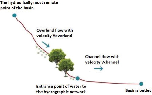
Figure 2. ArcGIS model for river delineation and spatial calculations in Model Builder.

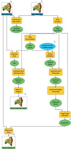
Figure 3. Reach-by-reach application of the computational procedure at the Nedontas River basin, for P_e = 10 mm.

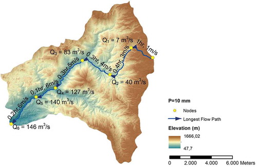
Figure 4. Locations of Mediterranean study catchments.

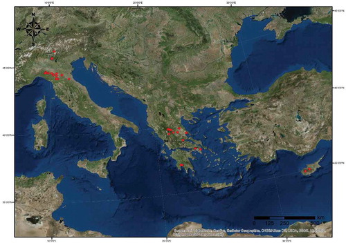
Figure 5. Estimated and simulated time of concentration as a function of runoff intensity for the basins of Nedontas (left) and Enipeus (right).

Figure 6. Different discretization approaches for the Titarisios River basin, considering 6, 12 and 19 junctions across the longest flow path.

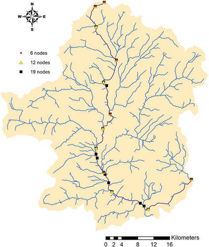
Figure 7. Comparison of actual (i.e. estimated through the GIS procedure) and simulated (by the corresponding regional formulas) parameters t₀ (left) and β (right).

Figure 8. Comparison of scatter plots published by Grimaldi et al. (2012) and the theoretical model (continuous line) derived through the empirical formula (Equation (6)).

Figure 9. Comparison of unit time of concentration values across study basins calculated with the empirical formula of Papadakis-Kazan (1987) and by the regional formula (Equation (6)).

4.4 Theoretical interpretation of parameters t₀ and β

Equation (6) is consistent with the studies reported in the literature, including theoretical and experimental relationships reported (cf. Table 2), as well as the observed hydrograph data provided by Grimaldi et al. (2012).

In the aforementioned relationship, the coefficient t₀ denotes a characteristic travel time of the basin that corresponds to a unit runoff depth, i_e = 1.0 mm h⁻¹. Herein, this will be referred to as unit time of concentration. As shown in Table 4, within the examined sample, t₀ ranges from 1.4 to 7.6 h (4.0 h, on average). Its value is systematically lower than the time of concentration estimated through the Giandotti formula, and generally higher than the value provided by the Kirpich formula.

In contrast, the exponent β of Equation (6) is a recession parameter, for which there are quite different findings in the literature. It is well known, according to the kinematic wave theory, that, combined with Manning’s formula, this exponent should theoretically range from 0.25, for triangular channels, to 0.40, for overland flow and wide rectangular channels. However, Saghafian et al. (2002), who applied a cell-by-cell approach to rectangular channels, estimated an exponent of 0.35, which is lower than the theoretical value of 0.40; this difference was attributed to the existence of a non-wide channel network in their study basin. Meyersohn (2016) commented that natural channels will not exactly follow the power relationship. Other researchers, who attempted to establish recession relationships for the lag time of the basin, have found exponent values much closer to ours. In particular, in a sample of five pasture basins in Australia, Askew (1970) estimated exponents ranging from 0.190 to 0.305, before proposing the use of a constant value of 0.230. It is also interesting that Askew (1970) failed to associate the exponents to the channel characteristics, and commented that this may indicate that simplifying the computation of the theoretical exponents can lead to incongruences between hydrology and hydraulics. Finally, Aron et al. (1991) and Loukas and Quick (1996) also tried to relate the lag time with the effective rainfall intensity, concluding with a negative power-law function with exponents equal to 0.25 and 0.20, respectively.

In our sample, the exponent β varies from 0.126 to 0.264 (0.206 on average), thus being within the large range of the associated values that are reported in the literature. Remember that that in our methodology rectangular channels are assumed, in an attempt to provide a parsimonious and, simultaneously, realistic, model structure. The exponents found here deviate significantly from the theoretical value of 0.40, which is, however, valid for wide shallow flow in rectangular channels. Apparently, for runoff depths up to 100 mm applied to generally narrow channels, the flow will definitely not be shallow, thus justifying the derivation of β values much lower than 0.40.

4.5 Sensitivity analysis

Initially, we investigated alternative schematizations of the Titarisios River basin, with respect to the model configuration reported so far (herein referred to as the “base” scenario), comprising 12 junctions across the longest flow path, in order to evaluate the effects of the level of discretization on the model outcomes. In particular, a rough discretization was employed, by assigning a coarser flow accumulation threshold, which resulted in only six junctions (i.e. half of the base scenario), as well as a quite detailed discretization, comprising 19 junctions (Fig. 6). Then, calculations were repeated to obtain the regression parameters t₀ and β. As shown in Table 6, the unit time of concentration is quite overestimated, by considering too rough a discretization, while the sensitivity of the exponent β is generally low. As expected, according to the theoretical justification discussed in Section 3.4, the implementation of a too detailed spatial analysis, in terms of number of junctions and associated sub-catchments, has negligible impacts on the model outcomes and thus the parameter values.

Table 6. Sensitivity analysis of the river discretization by means of variation of parameters t₀ and β at Titarisios River basin, with respect to their “base” number of junctions, N = 12.

	N = 6	N = 12	N = 19
t0 (h)	6.96	5.93	5.94
β	0.238	0.220	0.219

Taking as example the river basin of the Scoltenna upstream of Pievepelago, we next investigated the sensitivity of the model against variations of the two roughness components, k and n, which are quite challenging to determine on the basis of field observations, and even more through remote information (e.g. satellite maps). In this context, we changed the typical values k = 1.55, n = 0.033 and the segment widths of the test basin by 10 and 30%, repeated the calculations of the time of concentration as a function of runoff depth, and re-calculated the parameters t₀ and β. The results are summarized in Tables 7 and 8, respectively.

Table 7. Sensitivity analysis of surface roughness coefficients by means of variation of parameters t₀ and β at Scoltenna with respect to the “base” value, k = 1.55.

	–30%	–10%	Base value	+10%	+30%
t0 (h)	2.95	2.60	2.47	2.37	2.20
β	0.158	0.170	0.176	0.180	0.188

Table 8. Sensitivity analysis of Manning’s roughness coefficient by means of variation of parameters t₀ and β at Scoltenna with respect to the “base” value, n = 0.033.

	–30%	–10%	Base value	+10%	+30%
t0 (h)	2.18	2.38	2.47	2.56	2.72
β	0.158	0.170	0.176	0.180	0.188

In general, the relative impact of changing t₀ and β with respect to their base values, i.e. t₀ = 2.47 h and β = –0.176, is smaller than the relative change of the three input parameters. The surface roughness coefficient, k, is more sensitive than Manning’s roughness coefficient, n, and the river width. Moreover, the change of n results in systematically decreasing, up to negligible, changes in the time of concentration estimations, as the runoff intensity increases. The same applies for the sensitivity of the channel width, resulting in even more negligible changes (Table 9).

5 Regionalization of regression parameters

In essence, the proposed GIS approach is physically consistent and does not suffer from discretization issues when changing pixel size. However, despite its simplicity and much lower computational effort in comparison with raster-based approaches, it requires GIS facilities that are not always available (or may not be attractive) for everyday engineering purposes, and may also require some manual interventions within the determination of model inputs. For this reason, analytical formulas, such as the ones illustrated in Table 1, are strongly preferred by practitioners, who wish to employ fast and easy recipes, with minimal data requirements and negligible computational effort.

Since both parameters t₀ and β exhibit significant variability across the study catchments, we attempted to provide regional relationships, by expressing them as functions of abstract catchment properties. Initially, we investigated whether these parameters are correlated with the geomorphological characteristics given in Tables 3 and 4, and also looked for combinations of the above characteristics that ensure significantly high correlations. Next, different parameterizations were tested, each one calibrated against the results obtained by the application of the GIS procedure to the sample of 30 catchments. Finally, the optimized regional formulas were contrasted against existing literature approaches.

5.1 Correlation analysis

In our preliminary investigations, we computed the correlations between t₀ and β against the geomorphological characteristics of the basins (catchment area, A, length of longest flow path, L, average slope, J, width, b, and roughness coefficient, n, across the main stream), in an attempt to provide simple regression estimators of the two parameters. In this context, the Pearson correlation coefficients were used, employed for linear and power-type dependencies. The correlation values are summarized in Table 10.

Table 9. Sensitivity analysis of the channel widths by means of variation of parameters t₀ and β at Scoltenna with respect to the “base” value, b = 23.2 m.

	–30%	–10%	Base value	+10%	+30%
t0 (h)	2.28	2.41	2.47	2.53	2.63
β	0.162	0.172	0.176	0.179	0.185

Table 10. Linear and power-type correlations between parameters t₀ and β and the key geomorphological characteristics of study basins (catchment area, A, length of longest flow path, L, and average slope, J, width, b, and Manning’s coefficient, n, of the main stream), as well as the time of concentration estimations by Giandotti and Kirpich.

		A (km^2)	L (km)	J (%)	b (m)	n	tG (h)	tK (h)
t0 (h)	Linear	0.725	0.854	−0.789	0.337	−0.357	0.859	0.898
	Power	0.754	0.883	−0.931	0.463	−0.368	0.905	0.933
β	Linear	−0.378	−0.553	0.638	0.586	0.226	−0.532	−0.586
	Power	−0.508	−0.665	0.676	−0.587	0.227	−0.645	−0.694

This preliminary analysis indicated that the variability of both parameters is explained well by the length and slope of the main stream, and less by the drainage area and the average width of the main stream. These outcomes are reasonable. Indeed, as the maximum flow length, L, increases, the travel time, defined as the ratio of L to an average velocity across the longest flow path, also increases. This time is also an increasing function of the catchment area, A, because, in general, the larger the extent of the basin the larger the maximum flow length is expected to be. Regarding the average slope, J, this is a key factor in the hydraulic response of a river, affecting both the characteristic time parameter, t₀, and the exponent β, representing the recession of the travel time against the runoff intensity. The latter is also affected by the average width, b, of the main water course, which is a direct outcome of using Manning’s formula within hydraulic calculations.

5.2 Calibration framework

From Table 9, it is also observed that t₀ and β are highly correlated with the (constant) t_c values estimated by the Giandotti and Kirpich formulas, comprising combinations of the above geomorphological characteristics. Hence, we looked for composite expressions of t₀ and β that include these and additional characteristics, aiming to ensure, as much as possible, more accurate predictions of the two variables, while at the same time remaining as parsimonious as possible. Apart from fitting the base values of t₀ and β, given in Table 4, we aimed to reproduce the individual (i_e, t_c) pairs of Table 5, which are direct outcomes of the GIS-based computational procedure (remember that t₀ and β are processed data, estimated through regression).

In this context, a global optimization problem was formulated, by maximizing the Nash-Sutcliffe efficiency (NSE) between the actual and simulated t₀ and β values of the 30 study catchments, and minimizing the total square error between the actual and simulated t_c values (six per catchment, 180 in total).

After testing a large number of combinations, the following expression for the unit time of concentration, t₀ (h) was obtained:

(7)

where A is the catchment area (km²), L is the length of the longest flow path (km), b is the average width across the main water course (m), J is the average slope across the main water course (m m⁻¹) and n is the average Manning’s roughness coefficient. This relationship ensures very satisfactory prediction of the actual t₀ values, as shown in Figure 7 (left), as the optimized NSE value is 0.923.

The optimized expression for the exponent is:

(8)

which ensures an efficiency of 0.750. In the above relationship, the right-hand term expresses the deviation from the theoretical upper value β = 0.40, which stands for shallow flow conditions over a flat bed of infinite width. From Equation (8) we conclude that this deviation is explained by the catchment area, A, which is a measure of the discharge that enters the main water course, and the channel geometry, expressed by the length, L, and the average width, b. The wider the channel, the smaller will be the deviation from the theoretical limit. We remark that most of the empirical relationships developed so far consider this parameter as constant, with the exception of Askew (1970), who attempted to express the exponent β as a function of A and L. However, since the available data sample was too small (five catchments), he did not recommend the use of his formula.

Following the Rational method assumptions, i.e. Q = i_e A, an empirical relationship to associate the time of concentration as function of the peak discharge at the basin outlet can also be extracted:

(9)

Therefore, the time of concentration can alternatively be expressed as a negative power function of the peak discharge, also controlled by the exponent, β.

5.3 Comparison with literature approaches

Since the time of concentration is a theoretical quantity, referring to ideal conditions (i.e. uniform effective rainfall), a direct estimation of t_c on the basis of observed hydrological data is not possible. Consequently, it is not possible to establish a formal (i.e. data-based) validation procedure for evaluating the predictive capacity of Equation (6), parameterized through the regional formulas (7) and (8). In this context, our validations were based only on comparisons against literature approaches, which are also subject to uncertainties and inaccuracies. In particular, we compared our outcomes with the processed flood data by Grimaldi et al. (2012), the theoretical formula by Meyersohn (2016), and the semi-empirical formula by Papadakis and Kazan (1987).

Grimaldi et al. (2012) investigated dozens of observed rainfall–runoff events from four small-to-medium scale basins in the USA (Cow Bayou, North Creek, Escondido Creek and North Elm Creek) and demonstrated that the time of concentration varies significantly for different peak discharge values. Within data processing, the authors employed a recursive filter to isolate the direct runoff and the SCS-CN method to extract the effective from the gross rainfall. To our knowledge, their analysis is unique as it provides such a clear picture of the variability of t_c against observed runoff data. Their outcomes were compared against our empirical formula (Equation (6)), whose parameters were derived by the regional equations (7) and (8). The geomorphological characteristics of the four catchments and the derived t₀ and β values are given in Table 11. We remark that in the absence of related information, for the average channel width, reasonable values were assigned, accounting for the basin extent. As shown in Figure 8, in all catchments the empirical Q versus t_c relationship falls within the range of the observed data. Actually, it tends to match the most extreme observed events, namely the ones exhibiting the lowest response time with respect to the observed peak discharge, where surface flow obviously prevails. This is not surprising, since our methodology follows the Rational method assumptions, accounting exclusively for surface runoff and also ignoring routing processes over sub-catchments that result in attenuated peaks and increased response times.

Table 11. Catchment characteristics, source data, and estimated parameters t₀ and β within validation. Channel widths are approximately estimated.

River basin	Source data	A (km^2)	L (km)	J (%)	b (m)	n	(h)	β
Cow Bayou	Grimaldi et al. (2012)	13.1	7.4	5.9	15.0	0.04	3.05	0.221
North Creek	Grimaldi et al. (2012)	59.0	18.5	5.2	20.0	0.04	4.24	0.265
Escondido	Grimaldi et al. (2012)	22.8	8.6	2.9	15.0	0.04	4.58	0.216
North Elm Creek	Grimaldi et al. (2012)	119.5	35.4	1.4	25.0	0.04	9.76	0.297
Coyote Creek	Meyersohn (2016)	282.0	47.9	1.7	25.0	0.04	9.69	0.296

Meyersohn (2016) employed a variable flow velocity approach to compute the travel time and construct time–area curves for a range of excess rainfall intensities. This method was tested in a 282 km² gauged watershed in northern California, resulting in a similar relationship as Equation (6), with t₀ = 13.0 h and β = 0.294. By employing the proposed regional formulas (7) and (8), the values t₀ = 9.7 h and β = 0.296 were obtained (Table 11). We remark that the recession parameters are identical, yet in our approach the unit time of concentration is smaller by about 30%. This deviation is absolutely reasonable, since it is well known that a pixel-based approach provides larger response times with respect to channel-based approaches (Pavlovic and Moglen 2008). Furthermore, Meyersohn (2016) incorporated a flow routing algorithm, in order to account for basin storage effects. As already mentioned, such effects are not modelled in our method, thus resulting in faster responses.

Additional comparisons were made with the semi-empirical formula developed by Papadakis and Kazan (1987), for estimating the channel travel time across small catchments (Table 1). In Figure 9 we contrast the unit time of concentration estimated by the two approaches for the 30 study areas. As shown, the Papadakis-Kazan formula provides systematically higher t₀ values. However, in the small and medium catchments the deviations are rather small, while they become quite large as the catchment extent increases. This is reasonable, as the Papadakis-Kazan formula was developed on the basis of observed data extracted from very small basins (experimental set-ups and natural stream basins), with time of concentration values ranging within a couple of minutes. However, our regional formulas have been estimated by analysing a much larger extent of catchments, ranging over three orders of magnitude, i.e. from a few km² to more than 1000 km².

6 Conclusions

The time of concentration, t_c, one of the fundamentals of hydrology, and an essential input of most widespread engineering recipes, has reasonably been characterized as a paradox. The existence of multiple, ambiguous and even illogical definitions, as well as numerous formulas providing significantly different estimations, and, most importantly, its treatment as a constant of the basin rather than a variable quantity, has made t_c prone to severe misuse. In our work, we attempt to decode the paradox by taking into account the inherently dynamic behaviour of t_c, with its obvious dependence on the surface runoff generated in the basin.

Apparently, this is not a novel viewpoint. For many decades, there has been an ongoing discussion about the dependence of t_c (and the lag time) on rainfall (or runoff) rate, and several methodologies have been proposed, ranging from theoretical and empirical formulas to channel-based and, more often, raster-based computational procedures. However, many of these approaches are site-specific, while others (e.g. raster-based) are quite complicated and require several assumptions, which makes them less attractive for everyday practice. Moreover, they suffer from scaling issues, since the results are strongly affected by the pixel resolution. Finally, their physical consistency is questionable, since the velocity of each cell is independent of the velocity of the adjacent ones.

Our objective is to provide a generalized yet simple methodology, based on a consistent interpretation of t_c, as the travel time across the hydraulically more distant path (typically assumed identical to the longest flow path), for a given excess rainfall that is uniformly generated over the catchment. By discretizing this path into a relatively small number of sub-segments, and taking advantage of the well-known Rational method assumptions, we have developed a kinematic approach to estimate the flow velocity, and thus the travel time, from the headwater sub-catchment to the basin outlet. The preparation of (most of) model inputs and the computations have been automatized in a GIS environment. However, we emphasize that the implementation of the method should not be regarded as a black-box procedure, since several decisions are subject to engineering evidence; among them, the determination and configuration of the flow path up the headwater catchment, and the assignment of representative hydraulic properties and parameters to the modelling components (i.e. sub-reaches). This task is not straightforward, particularly in cases of long reaches with heterogeneous characteristics. Moreover, our analyses at specific basins indicated that the model sensitivity against its inputs is relatively small; however, more extended investigations have to be employed to extract safe conclusions.

By testing this methodology in a large number of Mediterranean basins, spanning from a few up to more than 1000 km², we have confirmed that the time of concentration is a negative power function of the runoff intensity. Taking advantage of the extended outcomes of our sample, we provide further insight into the two parameters of Equation (6), i.e. the unit time of concentration, t₀ (scale parameter), and the exponent, β, and their association with the abstract geomorphological characteristics of the catchment (area, longest flow path length, average slope, channel width and Manning’s roughness coefficient). Looking for an even simpler alternative for the analytical approach, we have developed the regional relationships (Equations (7) and (8)) for estimating t₀ and β, respectively, which have been validated against experimental data and existing theoretical and semi-empirical relationships.

Before closing this discussion, it is essential to be reminded that the time of concentration is only a theoretical quantity, which is valid under ideal conditions. In particular, we hypothesise a uniformly distributed surface runoff, which enters the main stream of the catchment at the inflow points (junctions), and uniform flow conditions across rectangular sub-reaches, where regulation and overbank flow processes are ignored. In fact, in the case of mild slopes, the routing mechanisms significantly affect the flow dynamics, resulting in larger response times and attenuated peak flows. Moreover, at each confluence junction we assume that the inlet time from each individual sub-catchment is by definition lower than the accumulated travel time across the upstream flow path. Yet, with few exceptions, this is a reasonable assumption, particularly when the extent of sub-catchments is relatively small and one moves downstream. In this context, the peak discharge given by Equation (1) should be interpreted carefully as a preliminary indicator of the catchment’s response under the aforementioned assumptions, but not be used for design purposes.

Nevertheless, implementing the concept of the varying time of concentration into practice still remains an open issue that needs to be addressed. In fact, this requires a major shift from the widespread yet flawed hypothesis of constant t_c, thus also drifting substantial elements of hydrological modelling. For instance, in the context of the Rational method, a key assumption is that the duration of design rainfall, d, should be at least as long as the t_c, thus ensuring that the whole basin is contributing to runoff at the catchment outlet. If t_c is known a priori (e.g. through an empirical formula that merely accounts for the basin characteristics), the critical rainfall intensity, i, for the return period of interest, T, is estimated by the idf expression, i.e. a function of the form i = f(d, T), by setting d = t_c. However, by considering t_c as a function of the effective rainfall, i.e. the product ci, the rational formula cannot be solved explicitly, thus requiring few iterations in the estimate to converge to a constant value of rainfall duration and, consequently, a constant peak discharge (cf. Efstratiadis et al. 2014).

The implementation of a varying time of concentration is easier in the context of continuous modelling, where extraction of the effective from the gross rainfall does not (and should not) depend on the value of t_c. Actually, the reasonable dependence of the catchment’s response time on the runoff produced over its surface cannot only affect the spatiotemporal propagation of runoff. In everyday engineering practice, this is typically represented in a lumped manner, through the unit hydrograph theory. The dynamic unit hydrograph, the shape of which follows the variability of the excess rainfall intensity, is an evident consequence of the rainfall-dependent time of concentration, and an essential component of this new working paradigm. Ongoing research indicates that the adaptation of the varying t_c within well-known modelling approaches is not a cumbersome task, and can ensure physically consistency and thus reliable estimations in the context of hydrological design and flood risk evaluations. The outcomes of this research will be reported in due course.

Acknowledgements

The authors are grateful to Salvatore Grimaldi, Andrea Petroselli and Flavia Tauro for providing the data used within Section 5.3, as well as their kind comments, and the two anonymous reviewers for their fruitful comments and suggestions that helped us improve this article.

Disclosure statement

No potential conflict of interest was reported by the authors.

References

- Antoniadi, S., 2016. Investigation of the river basin’s response time variability. Postgraduate thesis. Department of Water Resources and Environmental Engineering, National Technical University of Athens full text and extended English abstract are Available from: http://www.itia.ntua.gr/1639/.
- Aron, G., Ball, J.E., and Smith, T.A., 1991. Fractal concept used in time-of-concentration estimates. Journal of Irrigation and Drainage Engineering, 117 (5), 635–641. doi:10.1061/(ASCE)0733-9437(1991)117:5(635)
- Askew, A.J., 1970. Derivation of formulae for variable lag time. Journal of Hydrology, 10 (3), 225–242. doi:10.1016/0022-1694(70)90251-9
- Corps of Engineers, 1954. Airfield drainage investigation. Washington, DC: U.S. Army, Los Angeles District for the Office of the Chief of Engineers, Airfield Branch Engineering Division, Military Construction, Data Report.
- Cronshey, R., 1986. Urban hydrology for small watersheds. Washington, DC: US Dept. of Agriculture, Soil Conservation Service, Engineering Division.
- Dietrich, W.E., et al., 1993. Analysis of erosion thresholds, channel networks and landscape morphology using a digital terrain model. The Journal of Geology, 101, 259–278. doi:10.1086/648220
- Efstratiadis, A., et al., 2014. Flood design recipes vs. reality: can predictions for ungauged basins be trusted? Natural Hazards and Earth System Sciences, 14 (6), 1417–1428. doi:10.5194/nhess-14-1417-2014
- Gericke, O.J. and Smithers, J.C., 2014. Review of methods used to estimate catchment response time for the purpose of peak discharge estimation. Hydrological Sciences Journal, 59 (11), 1935–1971. doi:10.1080/02626667.2013.866712
- Giandotti, M., 1934. Previsione delle piene e delle magre dei corsi d’acqua, Memorie e Studi Idrografici. Roma: Ministero dei Lavori Pubblici.
- Grimaldi, S., et al., 2010. Flow time estimation with spatially variable hillslope velocity in ungauged basins. Advances in Water Resources, 33 (10), 1216–1223. doi:10.1016/j.advwatres.2010.06.003
- Grimaldi, S., et al., 2012. Time of concentration: a paradox in modern hydrology. Hydrological Sciences Journal, 57 (2), 217–228. doi:10.1080/02626667.2011.644244
- Haan, C.T., Barfield, B.J., and Hayes, J.C., 1994. Design hydrology and sedimentology for small catchments. London: Academic Press.
- Izzard, C.F. and Hicks, W.I., 1946. Hydraulics of runoff from developed surfaces. In: 26th Annual Meetings of the Highway Research Board, 5–8 December, Washington, DC, 129–150.
- Kadoya, M. and Fukushima, A., 1977. Concentration time of flood runoff in smaller river basins. In: H.J. Morel-Seytoux, et al., eds. Proceedings of the 3rd International Hydrology Symposium on Theoretical and Applied Hydrology, 27–29 July, Fort Collins, CO. Fort Collins: Water Resources Publication, Colorado State University, 75–88.
- Kirpich, Z.P., 1940. Time of concentration of small agricultural watersheds. Civil Engineering, 10 (6), 362.
- Kjeldsen, T.R., et al., 2016. Evidence and implications of nonlinear flood response in a small mountainous watershed. Journal of Hydrologic Engineering, 21 (8), 04016024. doi:10.1061/(ASCE)HE.1943-5584.0001343
- Leopold, L.B. and Maddock Jr, T., 1953. The hydraulic geometry of stream channels and some geomorphologic implications. US Geological Survey Professional Papers, 252, 56.
- Loukas, A. and Quick, M.C., 1996. Physically-based estimation of lag time for forested mountainous watersheds. Hydrological Sciences Journal, 41 (1), 1–19. doi:10.1080/02626669609491475
- Maidment, D.R., et al., 1996. Unit hydrograph derived from a spatially distributed velocity field. Hydrological Processes, 10, 831–844. doi:10.1002/(SICI)1099-1085(199606)10:6<831::AID-HYP374>3.0.CO;2-N
- McCuen, R.H., 1989. Hydrologic analysis and design. Englewood Cliffs, NJ: Prentice Hall.
- McCuen, R.H., 2009. Uncertainty analyses of watershed time parameters. Journal of Hydrologic Engineering, 14 (5), 490–498. doi:10.1061/(ASCE)HE.1943-5584.0000011
- McNamara, J.P., et al., 2006. Channel head locations with respect to geomorphologic thresholds derived from a digital elevation model: a case study in northern Thailand. Forest Ecology and Management, 224 (1–2), 147–156. doi:10.1016/j.foreco.2005.12.014
- Meyersohn, W.D., 2016. Runoff prediction for dam safety evaluations based on variable time of concentration. Journal of Hydrologic Engineering, 21 (10), 04016031. doi:10.1061/(ASCE)HE.1943-5584.0001406
- Montgomery, D.R. and Dietrich, W.E., 1988. Where do channels begin? Nature, 336, 232–234. doi:10.1038/336232a0
- Montgomery, D.R. and Foufoula-Georgiou, E., 1993. Channel network source representation using digital elevation models. Water Resources Research, 29 (12), 3925–3934. doi:10.1029/93WR02463
- Morgali, J.R. and Linsley, R.K., 1965. Computer simulation of overland flow. Journal of Hydraulics Division ASCE, 91 (HY3), 81–100.
- NRCS (National Research Conservation Service), 2010. Time of concentration. In: National engineering handbook, Part 630 hydrology, chapter 15. Washington, DC: US Department of Agriculture.
- Papadakis, K.N. and Kazan, M.N., 1987. Time of concentration in small rural watersheds. In: Proceedings of the ASCE Engineering Hydrology Symposium. Williamsburg, VA: ASCE, 633–638.
- Pavlovic, S.B. and Moglen, G.E., 2008. Discretization issues in travel time calculation. Journal of Hydrologic Engineering, 13 (2), 71–79. doi:10.1061/(ASCE)1084-0699(2008)13:2(71)
- Rao, A.R. and Delleur, J.W., 1974. Instantaneous unit hydrographs, peak discharges and time lags in urban basins. Hydrological Sciences Bulletin, 19 (2), 185–198. doi:10.1080/02626667409493898
- Saghafian, B., Julien, P.Y., and Rajaie, H., 2002. Runoff hydrograph simulation based on time variable isochrone technique. Journal of Hydrology, 261 (1–4), 193–203. doi:10.1016/S0022-1694(02)00007-0
- Singh, V.P., 1976. Derivation of time of concentration. Journal of Hydrology, 30 (1–2), 147–165. doi:10.1016/0022-1694(76)90095-0
- Tarboton, D.G., Bras, R.L., and Rodriguez-Iturbe, I., 1991. On the extraction of channel networks from digital elevation data. Hydrological Processes, 5, 81–100. doi:10.1002/(ISSN)1099-1085
- Wong, T.S., 2005. Assessment of time of concentration formulas for overland flow. Journal of Irrigation and Drainage Engineering, 131 (4), 383–387. doi:10.1061/(ASCE)0733-9437(2005)131:4(383)
- Yu, B., et al., 2000. The relationship between runoff rate and lag time and the effects of surface treatments at the plot scale. Hydrological Sciences Journal, 45 (5), 709–726. doi:10.1080/02626660009492372