Multi-hydro hydrological modelling of a complex peri-urban catchment with storage basins comparing C-band and X-band radar rainfall data

ABSTRACT

The spread of impervious surfaces in urban areas combined with the rise in the intensity of rainfall events as a result of climate change has led to dangerous increases in storm water flows. This paper discusses a new implementation of the fully distributed hydrological model Multi-Hydro (developed at École des Ponts ParisTech), when operating storage basins, and its ability to deal with high-resolution radar rainfall data. The peri-urban area of Massy (south of Paris, France) was selected as a case study for having six of these drainage facilities, used extensively in flood control. Two radar rainfall datasets with different spatiotemporal resolutions were used: Météo-France’s PANTHER rainfall product (C-band) and ENPC’s X-band DPSRI. The rainfall spatiotemporal variability was analysed statistically using Universal Multifractals (UM). Finally, to validate the application, the water level simulations were compared with local measurements in the Cora storage basin located next to the catchment’s single outlet.

KEYWORDS:

• fully distributed model
• X-band radar
• rainfall
• spatiotemporal variability
• multifractals

Editor A. Castellarin Associate editor E. Rozos

1 Introduction

According to a survey published by the United Nations, 54% of the world’s population lived in urban areas in 2014, compared to 30% in 1950 (UN 2014). This increase has had a profound effect on land use and land cover, having a direct impact on the hydrological cycle and generating groundwater and watercourse pollution. Urban areas are among those most vulnerable to the impact of heavy rains (Kang et al. 1998, Schmitt et al. 2004, Chen et al. 2009). These concerns with urban hydrology drive the need to find environmental monitoring solutions and to promote efficient water resource management policies.

Improvement of the ability to measure and model hydro-meteorological events is therefore becoming more urgent, especially in (peri-)urban areas where high levels of imperviousness and smaller catchments lead to shorter response times (Berne et al. 2004, Segond et al. 2007, Ochoa-Rodrigues et al. 2015). Hence, there is great interest in the spatiotemporal resolution and reliability of the available data. With regard to obtaining rainfall data, weather radar has been widely used to address the scarcity of raingauge networks (Paz 2018), which provide local rainfall measurements. Although it does not perform direct rainfall measurements, radar provides space–time estimates of rainfall. Precipitation estimates are based on the measured reflectivity, which usually generates some uncertainties. However, for high rainfall intensity, dual polarization technology has been employed to improve the estimates of heavy rains (Bringi and Chandrasekar 2001, Illingworth and Blackman 2002). This technology uses the fact that large raindrops are flat (not spherical) and is based on the phase difference of the reflected (vertical and horizontal) signals to estimate precipitation rates directly.

Some authors have compared radar rainfall estimates with in situ measurements to try to validate the former (Tabary et al. 2011, Figueras I Ventura et al. 2012). Nevertheless, the intrinsic divergence between volumetric estimates carried out by radar and local measurements by raingauge make this direct comparison very complex (Ciach et al. 2003). An alternative, found to establish the validation and/or comparison of radar products, is the use of radar rainfall data in hydrological models, thus enabling the analysis of different responses (Berenguer et al. 2005, Ichiba 2016).

However, despite the availability of higher resolution distributed data (elevation, land use, rainfall, etc.), understanding water flows remains a challenge in the quest to grasp the hydrological behaviour of urban catchments. Indeed, the modelling of hydrological processes is intrinsically complex due to the heterogeneity of the areas and hydrological processes involved, and the interactions between them at various spatiotemporal scales. The difficulty of accurately defining an urban catchment, the permeability parameter uncertainties and the need to determine the real human impact on nature makes analysis even more difficult (Salvadore et al. 2015). In addition, because urban ground surfaces are characterized by a high degree of heterogeneity and imperviousness, rainfall data with fine spatiotemporal resolution are essential to develop an accurate model that can be validated and implemented (Fabry et al. 1994, Berne et al. 2004, Salvadore et al. 2015). Several studies have therefore been conducted to analyse the impact of the spatiotemporal variability of rainfall fields in urban areas on hydrological model response (Berne et al. 2004, Gires et al. 2012, Ochoa-Rodriguez et al. 2015, Paz et al. 2018). To take account of this detailed information on precipitation, high-resolution urban hydrological models have recently been developed and are increasingly applied (El-Tabach et al. 2009, Fewtrell et al. 2011, Giangola-Murzyn 2013, Pina et al. 2014, Ichiba 2016).

In addition, given that the Universal Multifractals (UM) approach (Schertzer and Lovejoy 1987) was developed specifically to deal with the extreme variability of rainfall fields over a wide range of scales, it was used here to statistically analyse the radar rainfall data, contributing to the comparison between C-band and X-band radar data.

The purpose of this study is to refine the Multi-Hydro model developed at École des Ponts ParisTech (see El-Tabach et al. 2009, for an initial version, Giangola-Murzyn 2013, Ichiba 2016). Multi-Hydro is a fully distributed hydrological model specifically designed for (peri-)urban areas.¹ Although the literature already includes extensive discussion of the hydrological modelling of urban and rural areas, Multi-Hydro can be used to model peri-urban areas, which is a particularly complex task (Giangola-Murzyn 2013). It is able to handle a high degree of heterogeneity and complex interactions between hydrological processes at different spatiotemporal scales, and to compare the hydrological results with C-band and X-band radar data. Earlier studies were carried out with this model using radar rainfall data (Gires et al. 2014, 2018, Ichiba et al. 2018), but none included or examined the operation of storage basins. Since these retention devices are known to be effective to control storm water runoff (Efstratiadis et al. 2008, Gaborit et al. 2013, Martin 2014), especially during strong rainfall events, this work aims to refine Multi-Hydro by incorporating storage basins into the model. This is therefore the first time (to the authors’ knowledge) that the operational impact of artificial storage basins has been modelled with Multi-Hydro. Massy, a peri-urbanized catchment in southwest Paris (France), was chosen as the case study for this purpose. In this paper, we discuss how the inclusion of storage basins introduces additional difficulties in the conceptualization of the hydrological system, notably by increasing the need for information and amplifying the uncertainties, ultimately requiring correction to the assumptions used in the model.

The paper is structured in five sections. Section 2 describes the case study and the Multi-Hydro model. The rainfall data and their UM analyses are presented in Section 3, and Section 4 discusses the results of the simulations. Finally, the conclusions are presented in Section 5.

2 Case study and modelling

2.1 Case study

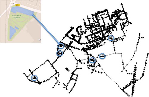
The catchment studied is part of the Bièvre River catchment managed by the Bièvre Valley Intermunicipal Sanitation Office (SIAVB; Syndicat Intercommunal d’Assainissement de la Vallée de la Bièvre), a local authority responsible for storm water management. This wider area encompasses 14 municipalities in a 110-km² peri-urbanized area to the southwest of Paris, France (Fig. 1). The upper Bièvre flows above ground from its source in St. Quentin (Department of Yvelines) to Antony (Department of Hauts-de-Seine), forming an approximately 18-km-long watercourse. This upstream section of the river and 15 km of its tributaries are inside the SIAVB zone. The Massy catchment studied herein is located in the downstream portion of the SIAVB catchment, in a 6.3-km² peri-urbanized area (Fig. 1).

Figure 1. Bièvre catchment, Massy sub-catchment, C-band radar and X-band radar locations.

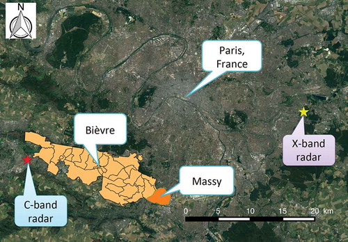
Since the Bièvre River is a tributary of the Seine River, it has been linked with major floods in Paris, such as that of January 1910. After severe floods in 1973 and 1982, the SIAVB decided to create a network of 15 storage basins across the upper Bièvre catchment in order to limit flooding. The operation of these basins is now remotely controlled and optimized at catchment scale during extreme events. Six of them are specifically located in the Massy sub-catchment.

2.2 Multi-Hydro

The fully distributed Multi-Hydro model (El-Tabach et al. 2009, Giangola-Murzyn 2013, Multi-Hydro 2015, Ichiba 2016) was developed in response to the lack of open source models able to account for the highly heterogeneous character of urban and peri-urban regions, as well as the need to carry out high-resolution modelling capable of representing spatiotemporal variability at different scales. It combines existing open source models, each separately representing part of the water cycle, so as to provide an interactive model of the full hydrological cycle within an urban environment. The models selected were: (i) the Two-Dimensional Run-off, Erosion and Export model (TREX; Velleux et al. 2011), a distributed model developed by Colorado State University, which models surface runoff, taking into account topography, land use and soil surface properties; (ii) the Variably Saturated 2-Dimensional flow and Solute Transport model (VS2DT; Lappala et al. 1987), a model used to calculate flows in unsaturated soil zones; and (iii) the Storm Water Management Model (SWMM; Rossman 2010), using only the hydraulic portion, which models water flows in the storm drain system. As each component is independent, Multi-Hydro has a modular structure that enables the user to adapt the interconnections between the components of an urban environment water cycle to the needs of each case study (Multi-Hydro 2015).

2.3 Data preparation: MH-AssimTool

In order to generate all the input data required by Multi-Hydro and to facilitate the handling of its scale changes, a geographic information system (GIS) based interface called MH-AssimTool was developed at École des Ponts (Richard et al. 2012). The inputs in this system are the topography, land use (including a gully class through which the link between the drainage module and the runoff surface is made), pedology, river network, catchment boundary and storm drain system. Except for topography, which is a raster text file, all other inputs are geospatial vector files (more precisely, files in shapefile – .shp – format). With this instrument, the geographical and physical information needed for modelling can easily be assimilated for each zone and resolution. MH-AssimTool generates three text files that are used as Multi-Hydro inputs: a land-use raster file (ASCII format) which presents the land use divided into categories at the desired spatial resolution; a file describing the storm drain system which can be imported into SWMM (.inp format); and a text file containing all the parameters needed for the simulation.

2.3.1 Land use

Information on land use was provided by the National Institute of Geographical and Forest Information (Institut National de l’Information Géographique et Forestière). The original land-use description contains 10 classes, which provide a detailed description of the catchment’s heterogeneity. However, as shown in Figure 2, the original data also contained many unidentified areas (with no land-use class) that required investigation.

Figure 2. Land use of Massy area with all available layers.

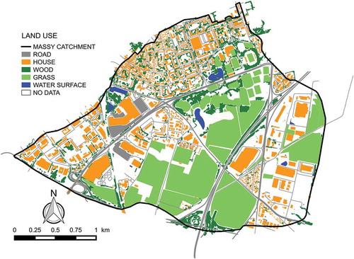
In order to fill in the missing information, the land-use data were processed using an open source GIS-based program, QGIS (http://www.qgis.org). The two layers representing roads (main and secondary) were originally composed of polylines that have not yet been integrated into MH-AssimTool. These layers were therefore buffered, i.e. an average width was assigned to these features (16 m for the main and 8 m for the secondary roads). Finally, only six land-use categories with different hydrological behaviours were retained: Gully, Road, House, Wood, Grass and Water Surface (parking areas, main and secondary roads were combined into the single “Road” class; and sports fields and farms into “Grass”).

The first phase in processing the land-use data was to complete the missing areas in the data and to verify the accuracy of the land-use distribution. A visual comparison was therefore performed between the data and Google satellite images using the QGIS software. First, some missing entities (in particular, houses and parking areas) identified in the images were added to the data to improve the land-use description. Then, the remaining areas were assumed to be covered with grass.

One of the chief advantages of using gridded models is their ability to represent catchment heterogeneity at the spatial resolution selected by the user to coincide with the purpose of the study, the availability of data and the required computation timescales. Indeed, Multi-Hydro has been used in several recent modelling studies (Gires et al. 2014, 2018, Versini et al. 2016, Ichiba et al. 2018), with spatial resolutions ranging from 100 m to 2 m. Our work employed a spatial resolution of 10 m, which retains most of the detail while maintaining an acceptable computational time.

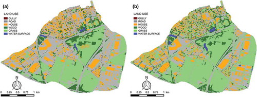
The first step in the implementation of the model is rasterization, i.e. allocating a single category of land use to each pixel in the domain. There are two different methods of performing this operation using MH-AssimTool (Ichiba et al. 2018). The first is based on the order of priority of the six land-use categories listed above, from the most to the least permeable. Since roads and houses are assigned a higher priority than grass and woods, this method of allocating land use obviously leads to the impervious surfaces being overestimated, which influences the hydrological behaviour of the catchment and therefore the simulation results, especially at larger pixels from bigger scales. However, it maintains the continuity of the roads and therefore the preferential water paths. The only way to reduce the impact of this overestimation problem is to use smaller pixels, which is only possible with high-quality data and more (potentially much more) computation time.

Ichiba (2016) proposed an alternative approach based on a pixel majority rule, which means that the class of each pixel is determined by the dominant land-use class observed within it. Thus, a process is implemented once the “Gully” pixels have first been allocated. The two methods of data rasterization were compared by Ichiba et al. (2018), whose results indicate that applying the majority rather than the priority order rule leads to a much better representation of catchment heterogeneity.

Figure 3 shows a comparison between the land-use maps obtained for the Massy catchment by applying the two methods discussed above with MH-AssimTool. The hydrological modelling results produced in this work involve both methods and both sets of results will be discussed.

Figure 3. Land use of Massy area: (a) with priority and (b) without priority order.

2.3.2 Storm drain system

Data on the storm drain system and storage basins were initially provided by Veolia, which is responsible for storm water management operations in Massy. It is important to mention that quite substantial preliminary work was done on the storm drain system data to make them compatible with MH-AssimTool. This mainly concerned connecting pipes, inspection points and gullies, and the following modifications:

1. Some of the storm drain elements provided were totally disconnected from the main network. The hydrological contributions of such components were assessed, resulting either in the re-establishment of a connection or a simplification of the system.

2. As for the roads category, buffering was performed to make the gullies compatible with MH-AssimTool. For this, a radius was attributed to each gully location point, converting it into a surface.

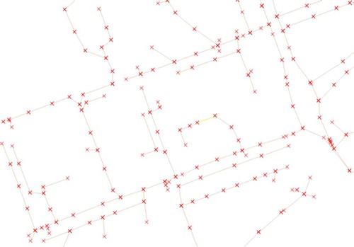
3. Some network connections were not single pipes, but rather a series of small pipe segments (Fig. 4), some of which had to be disconnected from the network. In this case, the QGIS command “Check geometry validity” – which verifies the shape relationship (topology), the shape location, the shape size and the shape credibility (see Wadembere and Ogao 2014 for more details) – was used to check whether a selected entity was a straight line and whether it was connected to the network. In this way, we were able to learn the number and type of errors and to correct them. This procedure was necessary to guarantee the water flow in the network during simulation.

Figure 4. Details of the storm drain system connections.

Once these corrections had been made, MH-AssimTool was run. However, as can be seen in Figure 5(a), the storm drain network generated by the program was still incomplete (e.g. missing information on pipes/gullies) or invalid in its geometry (e.g. storage basins and their associated devices). In order to complete the storm drain network, the GIS coordinates of gullies were compared with the equivalent coordinates in the SWMM file. The number of GIS available gullies was naturally higher than the number of gully dedicated pixels of 10 m × 10 m land-use data (see Fig. 5(a)). This difference occurred because two or more gullies may be co-located, i.e. they may be within the same pixel. It was therefore necessary to identify all such pixels, enabling the missing pipes to be added as well (Fig. 5(b)).

Figure 5. SWMM file of the storm drain system: (a) generated by MH-AssimTool and (b) later corrected.

Two additional difficulties were directly related to the quality of GIS data available. First, there was no diameter information on some of the pipes. In this case, the printed storm drain system maps provided by Veolia had to be used to add the right diameter values for all of them. Second, the GIS storm drain system input file had no information on the storage basins, which means they could not be included in the MH-AssimTool outputs (Fig. 5(a)). Six storage basins were manually inserted in the SWMM file (see Fig. 6).

Figure 6. SWMM file of the Massy sub-catchment and the six storage basins, with the Cora basin (measurement point) highlighted.

These storage basins are responsible for controlling flows in more vulnerable areas and at outlets. Their available characteristics are shown in Table 1, where D is the diameter of the storage basin orifice, H is the highest water level in the storage basin (above the lowest basin level) and Q (or Q_max) is the flow (or its maximum) in the respective downstream pipe. The Tuileries storage basin, which has two outlets, was divided into Tuileries A and Tuileries B. Each basin has inlets, which consist of pipes that channel water into the basin through gravity, and outlets that are orifice type flow regulators.

Table 1. Characteristics of the storage basins.

Storage basin	Area (m^2)	D (m)	h (m)	Q (m^3/s)
Privé	0.071	0.3	1.0	0.00127
Cora	0.196	0.5	1.5	0.3
Tuileries A	0.126	0.4	0.8	0.0702
Tuileries B	0.196	0.5	0.8	0.11
Georges B.	0.031	0.2	0.66	0.09
La Bonde	0.283	0.6	1.0	0.3
La Blanchette	0.071	0.3	0.9	0.081

2.4 Modelling of the storage basins

The hydrological modelling of complex urban catchments containing artificial storage basins and other regulatory devices required further developments to the Multi-Hydro model. In fact, by modifying the topography of a riverbed in TREX, the previous version of Multi-Hydro was already able to handle unregulated water bodies, but not the artificial storage basins found in Massy. The solution found was to add the artificial basins to the elements of the storm drain system in SWMM, while entirely ignoring them at surface level in the corresponding pixels in TREX. This required code changes in Multi-Hydro’s interacting core, since it handles information exchanges between surface processes (in TREX) and the storm drain network (in SWMM).

The discharge coefficients (Cd) of every orifice in the respective storage basin needed to be calculated before the simulation was performed, where Cd are dimensionless coefficients used to define the flow through the storage basin outlets. Thus, using the dataset shown in Table 1 and assuming total submersion, these coefficients could be estimated as follows (Rossman 2010):

(1) $\mathrm{C}\mathrm{d}=\frac{Q}{A.\sqrt{2g\left(h-h_o\right)}}$(1)

where $A=\frac{\pi D^2}{4}$ is the orifice cross-sectional area, h is the water level in the storage basin (above the lowest basin level), $g=9.81\mathrm{m}{\mathrm{s}}^{-2}$ is the standard acceleration under Earth’s gravity, and h_o is the height of the lowest level of the orifice relative to the lowest level of the basin.

For the Cora basin, h_o = 0 m. Veolia also provided the initial water levels, H₀, of the Cora basin for each of the rainfall events: H₀ = 0.039 m for the event of 12–13 September 2015, 0.596 m for 16 September 2015 and 0.071 m for 5–6 October 2015. Since the precise values of these two variables were missing for the other basins, h_o = 0 m was assumed for all the basins, yielding the discharge coefficients presented in Table 2. As regards the initial water levels, it was assumed that all the basins would overall present the same water level ratio – H₀/H – as the Cora basin. Table 2 presents the resulting H₀ values used for the three rainfall events.

Table 2. Discharge coefficients and initial water level in all storage basins for each of the three events studied.

		$H_0\left(\mathrm{m}\right)$
Storage basin	$\mathrm{C}\mathrm{d}$	12–13 September 2015	16 September 2015	5–6 October 2015
Privé	0.0041	0.026	0.397	0.047
Cora	0.2816	0.039	0.596	0.071
Tuileries A	0.1410	0.021	0.318	0.038
Tuileries B	0.1414	0.021	0.318	0.038
Georges B.	0.7961	0.017	0.262	0.031
La Bonde	0.2395	0.026	0.397	0.047
La Blanchette	0.2727	0.024	0.358	0.042

3 Rainfall data

3.1 Data description

After a particularly dry summer season in France, several heavy rainfall episodes were observed over the Bièvre Valley in September–October 2015. For this study, we selected three rainfall events, quite different but fairly typical of the region, which occurred on 12–13 September, 16 September and 5–6 October 2015. The precise timing (UTC) of the three events is reported in Table 3.

Table 3. Detailed timing (UTC), UM parameters, R² coefficients of the DTM estimates (for $q=1.5$ and $\eta =1$) and γ_S of the three events for the C-band and X-band radar data.

Event	Radar	Start time	Duration (h)	Time steps	α	C1	R^2	γS
12–13 September 2015	C-band	04:05	44	528 (5 min)	1.25	0.22	0.914	1.03
	X-band			773 (3.4 min)	1.54	0.18	0.913	1.07
16 September 2015	C-band	08:25	8.5	102 (5 min)	1.07	0.10	0.855	0.49
	X-band			149 (3.4 min)	1.46	0.10	0.886	0.70
5–6 October 2015	C-band	09:10	31	372 (5 min)	1.58	0.15	0.908	1.03
	X-band			545 (3.4 min)	1.79	0.15	0.931	1.11

To test the applicability of the new Multi-Hydro version, i.e. incorporating storage basins, and to study the hydrological impacts of small-scale rainfall variability for the Massy urban catchment, two radar datasets were used. The polarimetric C-band radar located in Trappes, about 22 km west of the catchment and operated by Météo-France, provided the first set of rainfall data. The polarimetric X-band radar installed by École des Ponts ParisTech (ENPC) on its campus, approximately 26 km east of the catchment, provided the second set of rainfall data.

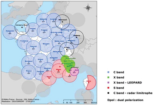
The spatial resolution of the C-band radar data is 1 km × 1 km, part of a mosaic of 29 radar facilities that covers the whole of France within the PANTHER project (Programme Aramis New Technologies Hydrometeorology Extension and Renewal, Parent-du-Châtelet 2003, Tabary 2007). However, as it is situated close to the study catchment, the Trappes C-band radar does not overlap with other radars in the Massy area, as shown in Figure 7. With regard to time resolution, the radar data estimate the incremental rainfall every 5 minutes.

Figure 7. The Météo-France radar network (©Météo-France).

It is important to emphasise that radars measure reflectivity rather than rain rate. The C-band radar data processing converts the reflectivity factor, $Z\left(\mathrm{m}{\mathrm{m}}^6{\mathrm{m}}^{-3}\right)$, into rain rate, $R\left(\mathrm{m}\mathrm{m}{\mathrm{h}}^{-1}\right)$, as follows (Marshall and Palmer 1948):

(2) $Z=a{R}^b$(2)

where a = 200 and b = 1.6 are fixed parameters for the Trappes C-band radar (Tabary 2007). The polarimetric function is used only to correct attenuation (Tabary et al. 2011).

The spatial resolution of the X-band radar data is 0.25 km × 0.25 km. The finest pixel resolution of the rainfall products was obtained by processing the radar radial measurements using standard Rainbow software (Selex 2015). In terms of time resolution, the X-band radar generates rainfall estimates every 3.4 min. The rainfall product used in this work is a Dual Polarization Surface Rainfall Intensity (DPSRI). This product makes full use of the X-band radar’s polarimetric capacities by employing differential reflectivity (ZDR) and specific differential phase (KDP). The radar data are pre-processed using Finite Impulse Response (FIR) filtering. For low rainfall intensities, the Z–R relationship is used, just as with the C-band radar, although with rather different parameters: a = 150 and b = 1.3. For higher intensities, $Z>35\mathrm{d}\mathrm{B}\mathrm{Z}\mathrm{a}\mathrm{n}\mathrm{d}\mathrm{K}\mathrm{D}\mathrm{P}>0.3\mathrm{d}\mathrm{e}\mathrm{g}/\mathrm{k}\mathrm{m}$, the following relationship was used:

(3) $R=19.63{\left|\mathrm{K}\mathrm{D}\mathrm{P}\right|}^{0.823}$(3)

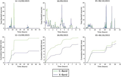
Figure 8 presents the accumulated rainfall per radar pixel for both C-band and X-band radars during the studied events. Figure 9 shows the time evolution of the average rain rate and cumulative rainfall depth, estimated for the whole Massy catchment. It can be seen that the X-band radar yields lower rainfall estimates. It is also apparent that finer pixel size provides much more detail in the detection of rainfall patterns.

Figure 8. Cumulative rainfall depths by radar pixels over the sub-catchment area, for both C-band and X-band radar data for the three events studied.

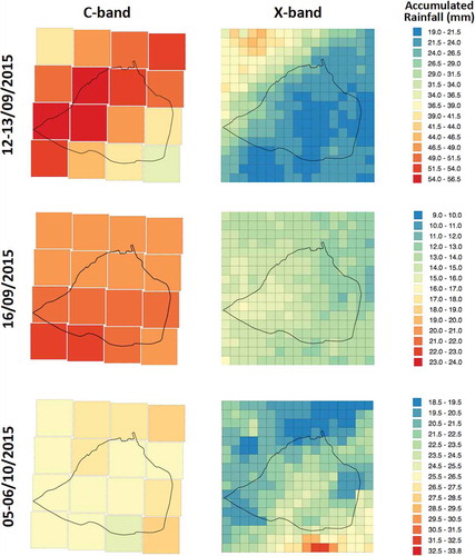
Figure 9. Time evolution of rain rate (top) and cumulative rainfall (bottom) over the whole sub-catchment area for the two data products (Météo-France C-band, in green; ENPC X-band, in blue) for the three events: 12–13 September 2015 (left), 16 September 2015 (centre) and 5–6 October 2015 (right).

3.2 Multifractal analysis

As highlighted again in Figures 8 and 9, the rainfall fields exhibit extreme variability over a wide range of space–time scales. Multifractals offer a convenient framework for the statistical quantification of this variability across scales (Schertzer and Lovejoy 1987, Tessier et al. 1993, Marsan et al. 1996, De Lima and Grasman 1999, Deidda 2000, Veneziano et al. 2006, Macor et al. 2007, Tchiguirinskaia et al. 2011, Gires et al. 2014, Tan and Gan 2017, Paz et al. 2018). The multifractal methodology relies on the concept of scale invariance and assumes that the rainfall field ($R_{\lambda }\propto {\lambda }^{\gamma }$), which is defined at a resolution $\lambda =L/l$ (where L is the largest scale of the field and l the observation scale) and characterized by the singularity γ (independent of the resolution), is generated through an underlying cascade process.

Furthermore, the multifractal field can be statistically described by two bi-univocally related functions (Parisi and Frisch 1985) – K(q) and c(γ) – defined as (Schertzer and Lovejoy 1987):

(4) $⟨{\epsilon }_{\lambda }^q⟩\approx {\lambda }^{K\left(q\right)}$(4)

(5) $\mathrm{P}\mathrm{r}\left({\epsilon }_{\lambda }\ge {\lambda }^{\gamma }\right)={\lambda }^{-c\left(\gamma \right)}$(5)

where < . > means global mathematical average and ≈ means the asymptotic equivalence; K(q) is the scaling moments function; and $c\left(\gamma \right)=D-d\left(\gamma \right)$ is the codimension function, D is the dimension of the domain and d(γ) is the fractal dimension function of the singularity.

Schertzer and Lovejoy (1987) developed the specific framework of Universal Multifractals (UM), where, based on turbulent systems (using cascade multiplicative processes), the statistical properties of multifractal processes can be defined using only three parameters, all with physical meaning:

• C₁, the mean intermittency codimension, which measures the intermittency (or concentration) of the average field. In other words, C₁ is the codimension of the mean singularity (C₁) for a conservative field: $C_1=c\left(C_1\right)$. Therefore, for a homogeneous field, $C_1=0$.

• $\alpha ϵ\left[0,2\right]$, the multifractality index (or Lévy index), which measures how the intermittency varies with the intensity level. For a monofractal case, $\alpha =0$.

• H, the Hurst exponent, which measures the degree of non-conservation of the field. For a conservative field, $H=0$.

Therefore, in the specific case of conservative UM, the statistical functions K(q) and c(γ) are described as:

(6) $K\left(q\right)=\left\{\begin{array}{c}\frac{C_1}{\alpha -1}\left(q^{\alpha }-q\right),\alpha \ne 1\\ C_{1}qlog\left(q\right),\alpha =1\end{array}\right.$(6)

(7) $c\left(\gamma \right)=\left\{\begin{array}{c}{C}_1{\left(\frac{\gamma }{C_1{\alpha }^{\prime }}+\frac{1}{\alpha }\right)}^{\frac{\alpha }{\alpha -1}},\alpha \ne 1\\ C_1{e}^{\left(\frac{\gamma }{C_1}-1\right)},\alpha =1\end{array}\right.$(7)

When the values of the parameters α and C₁ are both high, it indicates greater extremes. In order to estimate these statistical parameters for both X-band and C-band radar data, the Double Trace Moment (DTM) method (Lavallée et al. 1993) was applied to the time ensemble average over the full rainfall events (each time step being considered an independent realization). The results obtained for the three events studied, over a 64 km × 64 km area, are presented in Table 3. The α values for the C-band radar data are smaller than those obtained for the X-band radar data for all three events. For the last two events (16 September and 5–6 October 2015), the C₁ values are similar for the C-band and the X-band radar data. Together, these results suggest that X-band rainfall data exhibit multifractal patterns with stronger extremes. However, for the 12–13 September 2015 event, the conclusion is not straightforward, since C₁ obtained for the C-band radar data is greater than that obtained for the X-band radar data, while the α value is smaller. It is worth noting that the R² coefficients of the DTM estimates (also presented in Table 3), which provide an indication of the quality of the scaling, are similar for the C- and X-band radar data in the first event, and slightly smaller for the C-band radar data in the last two events. For the event of 16 September, these coefficients are less than 0.9 for both C- and X-band radar data, which implies greater uncertainties in the multifractal estimates.

The notion of maximum observable singularity (Hubert et al. 1993, Royer et al. 2008), γ_S, can also be used to analyse the data further. It combines the influence of both parameters α and C₁ (Schertzer and Lovejoy 2011) and can be linked to the maximum rainfall value:

(8a) ${\gamma }_S=\frac{\alpha }{\alpha -1}{C}_1{\left(\frac{D+D_S}{C_1}\right)}^{\frac{\alpha -1}{\alpha }}-\frac{C_1}{\alpha -1},\mathrm{f}\mathrm{o}\mathrm{r}\alpha \ne 1$(8a)

(8b) $max\left(R_{\lambda }\right)\propto {\lambda }^{{\gamma }_S}$(8b)

(8c) $N_S={\lambda }^{D_S}$(8c)

where D is the dimension of the embedding space (D = 1 for time series and D = 2 for maps, as in this paper), D_S is the sampling dimension and N_S is the number of realizations.

As can be seen in Table 3, the singularity γ_S is consistently slightly lower for C-band than for X-band radar data, including the 12–13 September event, indicating greater variability in the X-band rainfall fields. For this event, the mean singularity C₁ is slightly higher for the C-band radar data, which also implies higher accumulated rainfall over the 64 km × 64 km area. Hence, a smaller value for the maximum singularity γ_S results from a smaller value of α, implying that the intermittency varies less as the intensity level declines. It is also apparent that, of the three events, the 16 September event yields singularities much weaker than the other two, which yield very similar estimates of γ_S, despite greater multifractality and smaller intermittency for the 5–6 October event. Given that the uncertainties in the estimates of the UM parameters are greater for this event, as previously indicated by the lower R² coefficients, this should be considered as a trend and not over-interpreted.

The overall consistency in the singularity estimates (considering both C₁ and γ_S) for C- and X-band radar data suggests that the X-band radar yields lower rainfall estimates, mainly because of a difference in linear pre-factors (see Equation (8b)), which do not influence the scaling behaviour.

3.3 Rainfall data input to the model

The rainfall data input to Multi-Hydro requires a time resolution of 1 min and the same spatial resolution as the land use (10 m × 10 m in this study), regardless of the rainfall data product. QGIS tools were used to perform the intersection between the mesh of the model and the meshes of both the X- and C-band radar data. These rainfall files are generated by calculating the contribution of each radar data pixel’s pluviometric index to the model pixels, as follows (Paz et al. 2018):

(9a) $R_{i_{\mathrm{M}\mathrm{H},}{j}_{\mathrm{M}\mathrm{H}}}=\frac{{\sum }_{i_X,j_X}{R}_{i_X,j_X}\left(A_{i_{\mathrm{M}\mathrm{H}},j_{\mathrm{M}\mathrm{H}}}\cap A_{i_X,j_X}\right)}{{\sum }_{i_X,j_X}\left(A_{i_{\mathrm{M}\mathrm{H}},j_{\mathrm{M}\mathrm{H}}}\cap A_{i_X,j_X}\right)}$(9a)

(9b) $R_{i_{\mathrm{M}\mathrm{H},}{j}_{\mathrm{M}\mathrm{H}}}=\frac{{\sum }_{i_C,j_C}{R}_{i_C,j_C}\left(A_{i_{\mathrm{M}\mathrm{H}},j_{\mathrm{M}\mathrm{H}}}\cap A_{i_C,j_C}\right)}{{\sum }_{i_C,j_C}\left(A_{i_{\mathrm{M}\mathrm{H}},j_{\mathrm{M}\mathrm{H}}}\cap A_{i_C,j_C}\right)}$(9b)

where: $R_{i_{\mathrm{M}\mathrm{H},}{j}_{\mathrm{M}\mathrm{H}}}$ is the rainfall rate calculated for each model pixel; $R_{i_X,j_X}$ is the rainfall rate obtained with the X-band radar product in one pixel of the data mesh; $R_{i_C,j_C}$ is the rainfall rate obtained with the C-band radar product in one pixel of the data mesh; $A_{i_{\mathrm{M}\mathrm{H}},j_{\mathrm{M}\mathrm{H}}}$, $A_{i_X,j_X}$ and $A_{i_C,j_C}$ are the pixel areas of, respectively, the model, and the X-band and the C-band radar data.

4 Simulation results

The simulations were carried out using the Multi-Hydro model for the three events analysed, employing the two different rainfall radar data products (Météo-France C-band and ENPC X-band) and the two methods of land-use data rasterization (priority order and majority rule). Figures 10, 11, 12 and 13 present the results of the simulations.

Figure 10. Comparison of water level obtained by simulations – using the calculated discharge coefficient and four variations (−50%, −25%, +25% and +50%) for the Cora basin – and measurements for the three events: (a) 12–13 September 2015, (b) 16 September 2015 and (c) 5–6 October 2015.

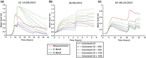
Figure 11. Time evolution of the difference in simulated water levels in Cora basin obtained with the highest (Cd + 50%) and the lowest (Cd − 50%) discharge coefficients used (top) and time evolution of the ratio of the same difference over the water levels in Cora basin obtained using the calculated Cd (bottom), for both radar data and for the three events studied: 12–13 September 2015 (left), 16 September 2015 (centre) and 5–6 October 2015 (right).

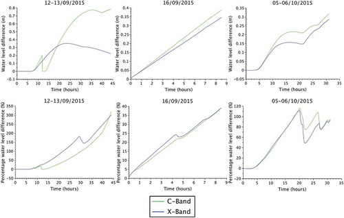
Figure 12. Comparison of water level in Cora basin obtained by simulations (using land use in the Massy area with priority and without priority order) and measurements for the three events: (a) 12–13 September 2015, (b) 16 September 2015 and (c) 5–6 October 2015.

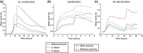
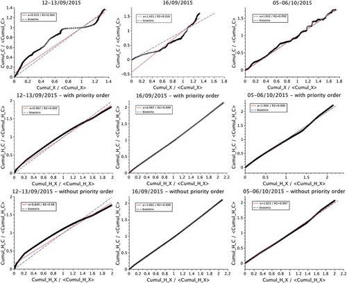
Figure 13. Relationships for cumulative total rainfall normalized by its mean (top), mean normalized cumulative water level using land use generated with priority order (centre), and mean normalized cumulative water level using land use generated without priority order (bottom), between C-band and X-band radars and three events: 12–13 September 2015 (left), 16 September 2015 (centre), 5–6 October 2015 (right). Continuous (red) line indicates the best linear fit, while the broken (blue) line corresponds to the first bisectrix.

In order to compare the time evolution of simulated water heights with the measured heights, Veolia provided a time series (every 5 min) of a water height point measurement in the Cora basin, located next to the catchment outlet (Fig. 6). The simulated water heights thus correspond to water volumes stored in the basin at each time step in the Multi-Hydro simulation (in SWMM module), normalized by the total area of the Cora basin (assuming vertical basin edges).

A comparison between the measured and simulated water level for different discharge coefficients (Cd) of the Cora basin (Fig. 10) demonstrates that the water level is heavily influenced by variations in this coefficient. For all three events studied, five different discharge coefficients were used in the sensitivity analysis: the first calculated using Equation (1), and the four others with a variation of $\pm 25\mathrm{\%}$ and $\pm 50\mathrm{\%}$ over the calculated value. Figure 10 shows that it is extremely important to have the correct value for the discharge coefficient parameter in a simulation, especially when there are multiple storage basins. As expected, when Cora’s discharge coefficient is reduced, the simulated water level increases, coming closer to the measurements during the first event for the X-band radar. However, the variations in Cd considered for the X-band radar rainfall are not sufficient to match the maximum water level measured during the 12–13 September event, whereas this level is significantly overestimated when the C-band radar rainfall is used. For the second event, varying Cd brings a degree of overlap between the simulations using the X-band rainfall and the measurements. However, the time evolution of the measured water level is more closely replicated when the C-band rainfall is used with Cd + 50%. Finally, for the third event, the variations in Cd considered are not sufficient to replicate the observations independently of the rainfall data source, although both closely track the time evolution of the measured water level. This discrepancy in the results could be due to the model’s sensitivity to the type of rainfall event (e.g. weak/strong), as well as to the absence of initial conditions (e.g. whether the soil is saturated or not), and should be even more pronounced when land use in the Massy area is modelled without the priority order.

Hence, Figure 11 displays the time evolution of the difference in simulated water levels obtained with the use of the highest (1.5Cd) and lowest (0.5Cd) discharge coefficients, and the percentage difference (defined as the previous quantity divided by the water level found when Cd is the discharge coefficient) for both sets of radar data of the Cora basin. With regards to the water level differences, the maximum level in the Cora basin for the 12–13 September event was reached about 13 hours after the start of the event for the C-band radar data input, and this naturally yields a water level difference falling to 0 m. For this event, the time evolution of this difference is significantly different for the two radar data inputs, with higher values reached for the C-band radar data. For the other two events, the difference examined exhibits similar patterns for both radar data inputs, with slightly greater values for the C-band data. This difference is reduced when percentages are studied (bottom row of Fig. 11). Except when the maximum level of the basin is reached, the values tend to increase during the rainfall event. In fact, this increase is almost linear for the 16 September event. The observed differences are not directly related to the event intensity. For example, the 16 September event is less intense than that of 5–6 October, but yields greater differences, though not so large in percentage terms. For the less intense event, the difference rises to 40%, which emphasises the high dependence of the output on the discharge coefficient.

Another comparison can be made between the water level measured in the Cora storage basin and the simulated water level, by reference to the two different land-use maps created (with either majority or priority rule) during the three events. It is observed (Fig. 12) that the more permeable land use created without the priority rule results in a larger drop in water level, for both the X-band and C-band radars, although generating greater uncertainties associated with unknown initial conditions. Moreover, this drop is more pronounced for the C-band data than for the X-band data (apparent for the 16 September and 5–6 October events). This highlights the model’s sensitivity to rainfall resolution, and therefore the need for a resolution as high as possible.

Finally, Figure 13 displays the nonlinear relations for the cumulative total rainfall normalized by its mean (top), for the normalized cumulative water level using land use generated with priority order (centre), and for the normalized cumulative water level using land use generated without priority order (bottom), between C-band and X-band radars during each of three events: 12–13 September 2015 (left), 16 September 2015 (centre) and 5–6 October 2015 (right). The purpose of using normalization by the corresponding mean was to highlight the nonlinearity of the time evolution of cumulative C- and X-band radar rainfall, and its influence on normalized cumulative water levels. While the cumulative rainfall measured by C-band radar remains higher than that measured by X-band radar for all three events (see Fig. 9), Figure 13 – which compares cumulative rainfall normalized by its mean – reveals significant differences between these three events.

For the event of 12–13 September 2015, the comparative curve convexity obtained for the time evolution of the cumulative rainfall below its mean (see the point of intersection of the curve with the bisectrix in Fig. 13) confirms a faster accumulation of C-band radar rainfall, which cannot be resolved by a simple pre-factor. This result differs from that obtained with the UM singularity γ_S computed through spatial analysis (see Section 3.2), but is more in agreement with the larger C₁ estimate. Two further points can be stressed. First, the spatial distribution of the C- and X-band radar data (and corresponding singularities) within the case study catchment becomes very local (e.g. over 4 × 4 pixels only for the C-band radar, see Fig. 8), and may differ significantly within the catchment compared with the total 64 km × 64 km area. This would explain why, with the X-band rainfall, the model does not reproduce the empirical water level maximum, which conversely is significantly overestimated with the C-band rainfall (see Fig. 10). Second, the difference in the linear pre-factor for the C- and X-band found in the spatial analysis could actually change over time. The convexity therefore propagates to the comparative graphs of normalized cumulative water levels and is more pronounced where land use is attributed by the majority rule. Conversely, the concavity of the comparative curve obtained for the cumulative rainfall below its mean confirms faster accumulation of X-band radar rainfall during the event of 16 September 2015. Hence, only a linear pre-factor triggers stronger cumulative C-band radar rainfall for this event, as discussed in Section 3.2. A smaller pre-factor seems to offset this faster accumulation, and the concavity of the comparative curves for normalized cumulative water levels disappears, regardless of which land-use attribution rule is used. Finally, for the event of 5–6 October 2015, all comparative curves show satisfactory linear behaviour. For this event, therefore, regardless of the source of the rainfall data, the simulations accurately reproduce the time evolution of the measured water level, although both fall short of the observed levels.

5 Conclusion

In this study, we first recalled the three main difficulties often faced when seeking to perform accurate hydrological modelling, i.e. data availability, data quality and data resolution. We illustrated some of the consequences of these issues for hydrological simulation with the Multi-Hydro model and discussed how its design helps to overcome the initial difficulties. In particular, by combining the results of a multifractal analysis of the radar rainfall data with the analysis of other hydrological quantities, we obtained a better understanding of simulation results, which at first glance could appear inconclusive. This improved understanding, in turn, validates (somewhat indirectly) the new developments to the Multi-Hydro model suggested here and promotes the exploitation of higher resolution radar rainfall in urban hydrology. This model has been specifically conceived to handle very heterogeneous fields and complex interactions among multifractal processes.

Unlike the semi-distributed conceptual models (e.g. InfoWorks CS, see Efstratiadis et al. 2008, Paz et al. 2018), which require exhaustive calibrations, the fully distributed physical models can better take into account the spatial variability of the data, as they use information (such as rainfall, topography, land use, etc.) distributed in regular grids of pixels of a given size. Multi-Hydro is designed in such a way that its spatial resolution can be optimized with regard to all the available data and to the scaling of urban hydrology flows. This is an innovative method of model resolution alteration that can replace the traditional model calibration methods (Ichiba et al. 2018). However, as demonstrated in this study, complete input data are required, especially in the case of a complex system such as a storm drain network, at least at a given scale. Furthermore, the effort to model the hydrology of a peri-urban catchment containing a number of regulation devices demanded new developments to the Multi-Hydro model. In this study, these storage capacities were directly incorporated into and executed by Multi-Hydro’s drainage module, where they are recognized as valid devices. This is the first time that the operative influence of such hydrological facilities has been modelled with Multi-Hydro. Two alternative rules, one based on priority order of land use, the other on pixel dominance (the so-called majority rule), were tested as a means of rasterizing land-use data. Both presented some advantages and disadvantages, which have been discussed in this work. The first method generates overestimated impervious surfaces, impacting on the hydrological results. This could be solved by using smaller pixels in the simulations, which would lead to more time-consuming simulations. On the other hand, it maintains the preferential water paths by keeping the continuity of the roads. The second method engenders a more realistic and more permeable land use. Nevertheless, the impacts of unknown initial conditions (such as soil saturation) become more relevant.

The lack of information about initial water level and orifice height for most of the basins (with the exception of Cora) made it impossible to establish precise initial conditions. In the absence of these data, a set of additional assumptions was proposed. This influenced the simulations, since the initial conditions of each basin alter the flow in the storm drain system and, consequently, the amount of water reaching the Cora basin (measurement point).

Overall, the simulations for three very different rainfall events showed that the Multi-Hydro model quite satisfactorily reproduces the time evolution of the water level in the Cora basin, e.g. accurately matching the peak regions, although it does not necessarily replicate the observed water levels. Indeed, we noticed that the X-band radar data consistently show lower water levels than the C-band radar data, often falling below the measured values. However, when the X-band and C-band radar data are compared, the absolute disparity between the simulated and measured water level values is lower with the X-band radar rainfall data in most of the analyses. We carefully analysed and presented a detailed account of the main possible reasons for this.

Acknowledgements

The authors would like to acknowledge partial support of the Chair of “Hydrology for Resilient Cities” endowed by Veolia, and of the Brazilian Army’s Department of Science and Technology. We also thank Bernard Urban (Météo-France) for providing access to the C-band radar data and the documentation within the framework of the INTERREG NWE RainGain project.

Disclosure statement

No potential conflict of interest was reported by the authors.

Additional information

Funding

This work was supported by the Brazilian Army’s Department of Science and Technology; INTERREG NWE RainGain project; Chair “Hydrology for Resilient Cities”;

Notes

¹ Here, peri-urban areas are defined as the transitional zones between fully urbanized and rural areas, generated by the expansion of big cities to a wider region, or “urban sprawl” (Rakodi 1998, Webster 2002, Schneider 2012).

References

- Berenguer, M., et al., 2005. Hydrological validation of a radar-based nowcasting technique. Journal of Hydrometeorology, 6 (4), 532–549. doi:10.1175/JHM433.1
- Berne, A., et al., 2004. Temporal and spatial resolution of rainfall measurements required for urban hydrology. Journal of Hydrology, 299, 166–179. doi:10.1016/S0022-1694(04)00363-4
- Bringi, V.N. and Chandrasekar, V., 2001. Polarimetric doppler weather radar: principles and applications. Cambridge, UK: Cambridge University Press.
- Chen, J., Arleen, A.H., and Lensyl, D.U., 2009. A GIS-based model for flood inundation. Journal of Hydrology, 373 (1–2), 184–192. doi:10.1016/j.jhydrol.2009.04.021
- Ciach, G.J., Habib, E., and Krajewski, W.F., 2003. Zero-covariance hypothesis in the error variance separation method of radar rainfall verification. Advancement Water Resources, 26, 573–580. doi:10.1016/S0309-1708(02)00163-X
- De Lima, M.I.P. and Grasman, J., 1999. Multifractal analysis of 15-min and daily rainfall from a semi-arid region in Portugal. Journal of Hydrology, 220, 1–31. doi:10.1016/S0022-1694(99)00053-0
- Deidda, R., 2000. Rainfall downscaling in a space-time multifractal framework. Water Resources Research, 36, 1779–1794. doi:10.1029/2000WR900038
- Efstratiadis, A., et al., 2008. HYDROGEIOS: A semi-distributed GIS-based hydrological model for modified river basins. Hydrology and Earth System Sciences, 12, 989–1006. doi:10.5194/hess-12-989-2008
- El-Tabach, E., et al., 2009. Multi-Hydro: a spatially distributed numerical model to assess and manage runoff processes in peri-urban watersheds. In: E. Pascheet, et al., eds. Final Conference of the COST Action C22, Road map towards a flood resilient urban environment. Paris, France: Hamburger Wasserbau-Schriftien.
- Fabry, F., et al., 1994. High resolution rainfall measurements by radar for very small basins: the sampling problem reexamined. Journal of Hydrology, 161, 415–428. doi:10.1016/0022-1694(94)90138-4
- Fewtrell, T.J., et al., 2011. Benchmarking urban flood models of varying complexity and scale using high resolution terrestrial LiDAR data. Physical Chemical Earth, Parts A/B/C 363 (7–8), 281–291. doi:10.1016/j.pce.2010.12.011
- Figueras I Ventura, J., et al., 2012. Long-term monitoring of French polarimetric radar data quality and evaluation of several polarimetric quantitative precipitation estimators in ideal conditions for operational implementation at C-band. Quaterly Journal of the Royal Meteorological Society, 138 (669), 2212–2228. doi:10.1002/qj.1934
- Gaborit, E., et al., 2013. Improving the performance of stormwater detention basins by real-time control using rainfall forecasts. Urban Water Journal, 10 (4), 230–246. doi:10.1080/1573062X.2012.726229
- Giangola-Murzyn, A., 2013. Modélisation et paramétrisation hydrologique de la ville, résilience aux inondations. Thesis (PhD). Université Paris-Est.
- Gires, A., et al., 2012. Quantifying the impact of small scale unmeasured rainfall variability on urban runoff through multifractal downscaling: a case study. Journal of Hydrology, 442, 117–128. doi:10.1016/j.jhydrol.2012.04.005
- Gires, A., et al., 2014. Impacts of small scale rainfall variability in urban areas: a case study with 1D and 1D/2D hydrological models in a multifractal framework. Urban Water Journal, 12 (8), 607–617. doi:10.1080/1573062X.2014.923917
- Gires, A., et al., 2018. Multifractal characterisation of a simulated surface flow: a case study with multi-hydro in Jouy-en-Josas, France. Journal of Hydrology, 558, 483–495. doi:10.1016/j.jhydrol.2018.01.062
- Hubert, P., et al., 1993. Multifractals and extreme rainfall events. Geophys Researcher Letters, 20, 931–934. doi:10.1029/93GL01245
- Ichiba, A., 2016. X-band radar data and predictive management in urban hydrology. Thesis (PhD). Université Paris-Est.
- Ichiba, A., et al., 2018. Scale effect challenges in urban hydrology highlighted with a distributed hydrological model. Hydrol Earth Systems Sciences, 22, 331–350. doi:10.5194/hess-22-331-2018
- Illingworth, A.J. and Blackman, T.M., 2002. The need to represent raindrop size spectra as normalized gamma distributions for the interpretation of polarization radar observations. Journal of Applied Meteorology, 41 (3), 286–297. doi:10.1175/1520-0450(2002)041<0286:TNTRRS>2.0.CO;2
- Kang, I.S., Park, J.I., and Singh, V.P., 1998. Effect of urbanization on runoff characteristics of the On-Cheon stream watershed in Pusan, Korea. Hydrol Processing, 12 (2), 351–363. doi:10.1002/(ISSN)1099-1085
- Lappala, E.G., Healy, R.W., and Weeks, E.P., 1987. Documentation of computer program VS2D to solve the equations of fluid flow in variably saturated porous media. U.S. Geological Survey Water-Resources Investigations Report 83-4099.
- Lavallée, D., et al., 1993. Nonlinear variability and landscape topography: analysis and simulation. In: L. De Cola and N. Lam, eds.. Fractals in geography. New Jersey: Prentice-Hall, 171–205.
- Macor, J., Schertzer, D., and Lovejoy, S., 2007. Multifractal methods applied to rain forecast using radar data. La Houille Blanche, 4, 92–98. doi:10.1051/lhb:2007052
- Marsan, D., Schertzer, D., and Lovejoy, S., 1996. Causal space-time multifractal processes: predictability and forecasting of rain fields. Journal of Geophysical Research, 101 (D21), 26,333–26,346. doi:10.1029/96JD01840
- Marshall, J.S., and Palmer, W.M.K., 1948. The distribution of raindrops with size. Journal of meteorology, 5 (4), 165–166. doi:10.1175/1520-0469(1948)005<0165:TDORWS>2.0.CO;2
- Martin, J., 2014. Remotely controlled sewers. Procedia Engineering, 70, 1084–1093. doi:10.1016/j.proeng.2014.02.120
- Multi-Hydro, 2015. ENPC, Agence de Protection des Programmes (APP) IDDN.FR.001.340017.000.S.C.2015.0000.31235.
- Ochoa-Rodriguez, S., et al., 2015. Impact of spatial and temporal resolution of rainfall inputs on urban hydrodynamic modeling outputs: a multi-catchment investigation. Journal of Hydrology, 531, 389–407. doi:10.1016/j.jhydrol.2015.05.035
- Parent-du-Châtelet, J., 2003. Aramis, le réseau français de radars pour la surveillance des précipitations. La Météorologie, 40, 44–52. doi:10.4267/2042/36263
- Parisi, G. and Frisch, U., 1985. A multifractal model of intermittency. Turbulence and predictability in geophysical fluid dynamics and climate dynamics. New York: North-Holland.
- Paz, I., et al., 2018. Multifractal comparison of reflectivity and polarimetric rainfall data from C- and X-Band radars and respective hydrological responses of a complex catchment model. Water, 10 (3), 269. doi:10.3390/w10030269
- Paz, I.S.R., 2018. Quantifying the rain heterogeneity by X-band radar measurements for improving flood forecasting. Thesis (PhD). Université Paris-Est.
- Pina, R., et al., 2014. Semi-distributed or fully distributed rainfall-runoff models for urban pluvial flood modelling? In: 13th international conference on urban drainage, ICUD2014, Sarawak, Malaysia.
- Rakodi, C., 1998. Review of the poverty relevance of the peri-urban interface production system research. Report for the DFID Natural Resources Systems Research Programme, 2nd Draft.
- Richard, J., et al., 2012. Advanced GIS data assimilation interface for evaluation of flood resilient systems. In: EGU General Assembly 2012, 22–27 April, Geophysical Research Abstracts, Vienna, Austria, 14352.
- Rossman, L.A., 2010. Storm water management model, user’s manual. Version 5.0. Cincinnati: U.S. Environmental Protection Agency, EPA/600/R-05/040.
- Royer, J.-F., et al., 2008. Multifractal analysis of the evolution of simulated precipitation over France in a climate scenario. C. R. Geosci., 340, 431–440. doi:10.1016/j.crte.2008.05.002
- Salvadore, E., Bronders, J., and Batelaan, O., 2015. Hydrological modelling of urbanized catchments: a review and future directions. Journal of Hydrology, 529, 62–81. doi:10.1016/j.jhydrol.2015.06.028
- Schertzer, D. and Lovejoy, S., 1987. Physical modelling and analysis of rain and clouds by anisotropic scaling multiplicative processes. Journal of Geophysical Research, 92, 9693–9714. doi:10.1029/JD092iD08p09693
- Schertzer, D., and Lovejoy, S., 2011. Multifractals, generalized scale invariance and complexity in geophysics. International Journal of Bifurcation and Chaos, 21 (12), 3417–3456. doi:10.1142/S0218127411030647
- Schmitt, T.G., Thomas, M., and Ettrich, N., 2004. Analysis and modeling of flooding in urban drainage systems. Journal of Hydrology, 299 (3–4), 300–311. doi:10.1016/S0022-1694(04)00374-9
- Schneider, A., 2012. Monitoring land cover change in urban and peri-urban areas using dense time stacks of Landsat satellite data and a data mining approach. Remote Sensing of Environment, 124, 689–704. doi:10.1016/j.rse.2012.06.006
- Segond, M.L., et al., 2007. Simulation and spatio-temporal disaggregation of multi-site rainfall data for urban drainage applications. Hydrol Sciences Journal – Journal Design Sciences Hydrol, 52 (5), 917–935. doi:10.1623/hysj.52.5.917
- Selex, 2015. Selex METEOR manual. Neuss: Selex ES GmbH.
- Tabary, P., 2007. The new french operational radar rainfall product. Part I: methodology. Weather Forecast., 22 (3), 393–408. doi:10.1175/WAF1004.1
- Tabary, P., et al., 2011. Evaluation of two “integrated” polarimetric Quantitative Precipitation Estimation (QPE) algorithms at C-band, Journal of Hydrology, 405 (3–4), 248–260. ISSN 0022-1694. doi:10.1016/j.jhydrol.2011.05.021
- Tan, X. and Gan, T.Y., 2017. Multifractality of Canadian precipitation and streamflow. International Journal Climatology, 37, 1221–1236. doi:10.1002/joc.5078
- Tchiguirinskaia, I., et al., 2011. Multifractal study of three storms with different dynamics over the Paris region. In: J. Moore, S. Cole, and A. Illingworth, eds. Proceedings of weather radar and hydrology. Exeter, United Kingdom: IAHS Publ., 351, 421–426. 18–21 April 2011.
- Tessier, Y., Lovejoy, S., and Schertzer, D., 1993. Universal multifractal: theory and observations for rain and clouds. Journal Applications Meteorl, 32 (2), 223–250. doi:10.1175/1520-0450(1993)032<0223:UMTAOF>2.0.CO;2
- United Nations, Department of Economic and Social Affairs, Population Division, 2014. World urbanization prospects: the 2014 Revision. [CD-ROM]. New York: United Nations.
- Velleux, M.L., England, J.F., and Julien, P.Y., 2011. TREX watershed modelling framework user’s manual: model theory and description. Fort Collins: Department of Civil Engineering, Colorado State University.
- Veneziano, D., Langousis, A., and Furcolo, P., 2006. Multifractality and rainfall extremes: a review. Water Resources Researcher, 42, W06D15. doi:10.1029/2005WR004716
- Versini, P.A., et al., 2016. Toward an operational tool to simulate green roof hydrological impact at the basin scale: a new version of the distributed rainfall-runoff model Multi-Hydro. Water Science and Technology : a Journal of the International Association on Water Pollution Research, 74 (8), 1845–1854. doi:10.2166/wst.2016.310
- Wadembere, I. and Ogao, P., 2014. Validation of GIS vector data during geo-spatial alignment. International Journal of Geoinformatics, 10 (4), 17–25.
- Webster, D.R., 2002. On the edge: shaping the future of peri-urban East Asia. Stanford, CA: Asia/Pacific Research Center Publication, Stanford University.