Intensity–duration–frequency curves exploiting neighbouring extreme precipitation data

ABSTRACT

Records of precipitation extremes are essential for hydrological design. In urban hydrology, intensity–duration–frequency curves are typically estimated from observation records. However, conventional approaches seldom consider the areal extent of events. If they do, duration-dependent area reduction factors are used, but precipitation is measured at only a few locations. Due to the high spatial variability of precipitation, it is relatively unlikely that a gauged observation network will capture the extremes that occur during a precipitation event. Therefore, the area reduction approach cannot be regarded as the reduction of an observed maximum. To investigate precipitation extremes, spatial aspects need to be considered using different approaches. Here, we both address the conventional practice of area reduction and consider a within-area chance of increased precipitation, defined as the maximum precipitation intensity observed in a cluster within a selected domain. The results show that (1) the risk of urban flooding is routinely underestimated in current design practice, and (2) traditional calculations underestimate extremes by as much as 30–50%. We show how they can be revised sensibly.

KEYWORDS:

• precipitation
• extremes
• area reduction factors
• intensity–duration curves

Editor S. Archfield Associate editor E. Volpi

1 Introduction

One of the early authoritative works on rainfall depth–area–duration analyses was published by the US Weather Bureau (1946). This was followed by work on intensity–duration–area–frequency studies ranging from 20 min to 24 h and from point data to 400 mi² areas, as reported in the series of four studies collated in the US Weather Bureau Technical Paper No. 29 (1960) as summarized by Chow (1964, Chapter 9). Bell (1976) added value to the 1975 Flood Studies Report (FSR) of the UK Natural Environment Research Council, wherein he developed meaningful procedures to improve the slightly muddled FSR calculations of area reduction factors (ARFs). He treated areas up to 1000 km² using Thiessen polygons based on raingauges and introduced a peak-over-threshold technique, fitting exponential distributions to the 20 highest daily values in those areas to determine intensity–duration–frequency (IDF) curves.

Temporal continuity of observations makes the assessment of IDFs popular. However, the consideration of the spatial aspect, which is essential for obtaining flood-producing volumes, is hampered by the lack of spatially continuous measurements. Stewart (1989) was among the first authors to combine gauge and radar data and found (as did Bell 1976) that ARFs reduce with increasing return periods. He worked with frontal and convective systems using 834 daily read gauges over 25 years in the UK over 544 catchments ranging from 5 to 100 km², so the problem was thoroughly researched. Burlando and Rosso (1996) developed methods for scaling what they called depth–duration–frequency (DDF) data, showing that simple scaling was not appropriate in many cases. They noted a break in the scaling slope at about 45 min duration, as was noted by Menabde et al. (1999).

Sivapalan and Blöschl (1998) used spatial correlation to obtain the parent distribution of catchment average rainfall intensity from the distribution of point rainfall intensity, through a variance reduction factor, and fitted a Gumbel distribution to the ARF curves. Krajewski et al. (2003) concluded that new designs of raingauge networks should be considered. In the process of their data collection and quality control, considerable evidence suggested that traditional networks based on single gauges cannot deliver reliable rainfall data, which is worrisome. More recently, Simonovic et al. (2016) stated that their primary objective was to standardize the IDF updating process and make the results of current research on climate change impacts on IDF curves accessible, which introduces a new variable into the mix. Bennett et al. (2016) introduced intensity–frequency–duration–area relationships for the consideration of the areal aspect of extremes.

In this paper, we ask the question: Are current applications of ARFs appropriate for urban design? Towns and cities are not catchments with a single outlet. They typically consist of many sub-catchments where the drainage system is determined by the storm water sewer network. Towns often have substantial areas (see Table 1) ranging from 10 to a few hundred square kilometres, so that extreme rainfall events may fall in only part of a town but can lead to substantial local damages. It is obvious that the probability that somewhere in London a 10-year return period precipitation depth will occur that is greater than the same return period precipitation occurring somewhere in Munich, due to their difference in area. In other words, the bigger the area, the greater the opportunity for a storm of a given size to occur.

Table 1. Areas currently covered by different cities.

Location	Area (km^2)
Berlin	891
Hamburg	755
Munich	310
London	1572

We investigate the influence of the size of the target urban area on the frequency of occurrence of extremes. We introduce two new concepts: (i) the maximum fall in a given interval over an area, and (ii) the sub-areal extremes. The properties of these are discussed in detail and we find that the space–time dependence of extremes strongly influences these statistics.

The study is divided into four complementary approaches. The first is to examine the records of a dense network of pluviometers covered by a radar in Baden-Württemberg, Germany, with a (regrettably) short 4-year record, as proof of concept, which illustrates the main points supporting our argument. The second approach is to use radar observations in the same area and time period. The third approach is to sample a long simulated sequence of radar rainfall fields of 1-km resolution to determine the statistics of a large plausible dataset. The procedure we used was to generate 20 years of “radar” fields of 5-min precipitation, including seasonality, on a frame of 128 × 128 1-km² pixels, and sample them in a regimented way. The extensive radar simulations were based on Gaussian spatial dependence, so in the fourth method we assessed the effect of modelling the rainfields with a more realistic chi-squared (χ²) spatial dependence, as suggested by Bárdossy (2006).

2 Methodology

To investigate precipitation extremes, the spatial aspect needs to be considered using approaches that are different from the conventional ones used previously. Besides the standard area reduction methods, we also consider a within-area chance of increased precipitation. This new measure is defined as the maximum precipitation intensity observed in a spatial cluster within a selected domain. The following quantities are defined mathematically, noting that the temporal integration in Equations (1)–(4) increments at the shortest successive observable time interval, not by the various periods of accumulation, ∆t. In other words, if the data are sampled at 5-min intervals, we accumulate them over that interval as well as a range of longer intervals up to 3 h, stepping forward by 5 min, so that we catch the maximum fall in a chosen interval during a rainfall event.

Figure 1 illustrates the ideas. The spatial labels are as follows: D is the domain of interest; x is the centroid of D; S is the location of heaviest precipitation at time t and aggregation interval ∆t in D and G_i is the ith sub-area of D. For the temporal integral labels: Z_A,D is the averaged areal precipitation over D; Z_L is the precipitation at the centroid of D; Z_S,D is the heaviest precipitation in D at site S, and Z_G,D is the heaviest precipitation in sub-area G_i, so that:

(i) Local maxima of precipitation totals for a duration ∆t at a selected gauge location x for a precipitation event are defined as:

(1) $Z_L\left(x,\mathrm{\Delta }t\right)=\underset{\tau }{\mathrm{m}\mathrm{a}\mathrm{x}}\left\{\underset{\tau }{\overset{\tau +\mathrm{\Delta }t}{\int }}Z\left(x,t\right)\mathrm{d}t\right\}$(1)

where Z(x,t) is the precipitation rate at a given site x and time t.

(ii) The maxima of areal total precipitation are defined on a domain D centred on x as:

(2) $Z_{A,D}\left(x,\mathrm{\Delta }t\right)=\underset{\tau }{\mathrm{m}\mathrm{a}\mathrm{x}}\left\{\underset{D}{\int }\underset{\tau }{\overset{\tau +\mathrm{\Delta }t}{\int }}Z\left(y,t\right)\mathrm{d}t\mathrm{d}y\right\}$(2)

(iii) While the previous two quantities are frequently used in practice, maximum precipitation intensity observed in the domain D is found to be:

(3) $Z_{S,D}\left(x,\mathrm{\Delta }t\right)=\underset{\tau ,y\in D}{\mathrm{m}\mathrm{a}\mathrm{x}}\left\{\underset{\tau }{\overset{\tau +\mathrm{\Delta }t}{\int }}Z\left(y,t\right)\mathrm{d}t\right\}$(3)

and is usually not considered. This quantity may be of importance for design, however. It reflects the usually unknown and neglected maximum within the domain of interest.

(iv) The fourth statistic for a set of sub-areas Gi ⊂ D for i = 1, …, I:

(4) $Z_{G,D}\left(x,\mathrm{\Delta }t\right)=\underset{i}{\mathrm{m}\mathrm{a}\mathrm{x}}\underset{\tau ,}{\mathrm{m}\mathrm{a}\mathrm{x}}\left\{\underset{G_i}{\int }\underset{\tau }{\overset{\tau +\mathrm{\Delta }t}{\int }}Z\left(y,t\right)\mathrm{d}t\mathrm{d}y\right\}$(4)

is thus the maximum amount of areal precipitation in sub-area G_i of D during time interval ∆t.

This last quantity is related to possible subscale floods in the area D, which may occur more frequently than in a selected sub-area.

The following relationships hold for these quantities:

(5) $Z_L\left(x,\mathrm{\Delta }t\right)\le Z_{S,D}\left(x,\mathrm{\Delta }t\right)$(5)

Then if D₁ ⊂ D₂:

(6) $Z_{S,D_1}\left(x,\mathrm{\Delta }t\right)\le Z_{S,D_2}\left(x,\mathrm{\Delta }t\right)$(6)

so both are by definition true. Frequently we have the situation where

(7) $Z_{A,D}\left(x,\mathrm{\Delta }t\right)\le Z_L\left(x,\mathrm{\Delta }t\right)$(7)

However, as the most intense precipitation corresponding to an areal event does not necessarily occur at x, there may be cases where the areal average precipitation exceeds the precipitation at the centre.

These quantities are calculated for each precipitation event in domain D defined by a separation of at least 6 dry hours. In this way temporal dependence between these quantities is avoided. As a next step, the maxima of these event statistics are calculated for the whole observation period. The resulting cumulative distributions are denoted as F_S,D,∆t(z), F_L,∆t(z), F_A,D,∆t(z) and F_G,D,∆t(z). For a given non-exceedence probability the conventional ARF is:

(8) $\mathrm{A}\mathrm{R}\mathrm{F}\left(D,\mathrm{\Delta }t\right)\left(p\right)=\frac{F_{A,D,\mathrm{\Delta }t}^{-1}\left(p\right)}{F_{L,\mathrm{\Delta }t}^{-1}\left(p\right)}$(8)

While areal extremes are of interest for discharges at the outlet of a catchment, maxima in a smaller neighbourhood may cause damage in sub-areas, thus they are also of interest for design.

All these quantities are closely related to the spatial dependence structure of extreme precipitation. In order to quantify dependence of extremes, the tail dependence of copulas of precipitation is usually calculated in practice (Aghakouchak et al. 2010). This approach, however, has the problem that it considers simultaneous occurrences, while we investigate extremes within events which do not necessarily match in segments of time within the event. Further it was demonstrated in Serinaldi et al. (2015) that the estimators of tail dependence are strongly influenced by non-extremes and thus are likely to be misleading.

Assuming that the precipitation spatial dependence is described using a multivariate copula, parameterized by the configuration for a chosen ∆t, one can write:

(9) $Z_{S,D}\left(x,\mathrm{\Delta }t\right)=\underset{x\in D}{\mathrm{s}\mathrm{u}\mathrm{p}}\left\{Z\left(x,\mathrm{\Delta }t\right)\right\}\approx \underset{i}{\mathrm{m}\mathrm{a}\mathrm{x}}\left\{Z\left(x_i,\mathrm{\Delta }t\right),i=1\dots n\right\}$(9)

where

(10) $\underset{i}{\mathrm{m}\mathrm{a}\mathrm{x}}\left\{Z\left(x_i,\mathrm{\Delta }t\right),i=1\dots n\right\}=F_Z^{-1}\left(\underset{i}{\mathrm{m}\mathrm{a}\mathrm{x}}\left\{U\left(x_i,\mathrm{\Delta }t\right),i=1\dots n\right\}\right)$(10)

where F_Z is the distribution of precipitation amounts and U (x_i, ∆t) = F_Z  {Z(x_i, ∆t)}. Thus the distribution of Z_S,D can be written as:

(11) $F_{Z_{S,D}}\left(z\right)=C_n\left(F_{Z_1}\left(z\right),\dots F_{Z_n}\left(z\right)\right)=C_n\left(F_Z\left(z\right),\dots F_Z\left(z\right)\right)$(11)

where C_n is the copula describing the spatial dependence of Z corresponding to points x_i.

3 Pluviometer data

In Baden-Württemberg, Germany, we have access to 38 months of pluviometer data (from May 2014 to July 2017) recorded in a relatively dense network in the town of Reutlingen. The network consists of 12 pluviometers recording at a time resolution of 5 min. Figure 2 shows the locations of the pluviometers, in an area that is approximately 25 km square. As these data cover more than the town area; we cannot determine the exact areal precipitation amounts, but we can see the differences in the distributions defined in Section 2, and these are shown as cumulative probability distributions (cdfs) in Figures 3 to 8.

The areal precipitation was calculated as the arithmetic average of the catch at the stations involved. Different configurations were considered. The evaluations were performed on the 20 largest averaged values of the corresponding distributions.

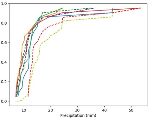
Figure 3 shows the distributions of the individual stations (solid lines) and some of the derived distributions at 5-min aggregations. One can see that:

• the four stations have practically the same extremes, except for the maxima, thus their average (blue dashed line) is a good representation of the distributions;

• the areal precipitation (green dashed line) is smaller, but not by very much;

• the maxima (red dashed line) are partly dependent, as the line shows higher values than the average, but there is some dependence as, under independence, the maxima would be on the olive line, which shows the distribution of the maxima when assuming that the stations are independent.

Figure 1. Explanation of the methodology. D is the domain of interest, X is the centroid of D, S is the location of heaviest precipitation in D and G_i is the ith sub-area of D. For the temporal integral labels, we define Z_A,D as the averaged areal precipitation over D, Z_L as the precipitation at the centroid of D, Z_S,D as the heaviest precipitation in D and Z_G,D as the heaviest precipitation within the ith sub-area G_i. (See online version for colour versions of figures that are not colour in print.)

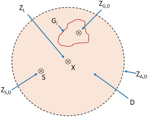
Figure 2. Pluviometer network of Reutlingen, Germany; the area is approximately 25 km square.

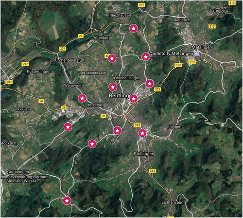
Figure 3. Distributions corresponding to the central four pluviometers in Figure 2 and the time aggregation of 1 h. Solid lines are the distributions of the individual stations, dashed lines are the distribution of the areal precipitation (green), the mean of the four distributions (blue), and the distribution of the maxima, Z_S,_D (red). The olive line shows the distribution of the maxima assuming that the stations are independent. The units on the horizontal axis are in mm and the vertical axis is cumulative probability.

When considering a bigger radius containing eight stations, the results change slightly. Figure 4 shows the distributions of the individual stations (solid lines) and some of the derived distributions, noting that the horizontal axes are the same as in Figure 3 with maxima of 57 mm. The red dashed line has moved away from the individual distributions towards the olive line, showing that there is less dependence if a larger area is considered.

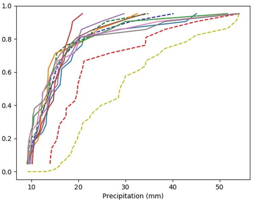
Figures 5 and 6 demonstrate the relationships for 15-min aggregations, the first using data from four pluviometers and the next using eight, while Figures 7 and 8 show the results for 3-h aggregations, which is the typical duration of an extremely heavy thunderstorm.

Figures 5–8 show that the frequency of extremes within a given area depends on its size and on the spatial dependence of precipitation. The limited number of stations does not allow the calculation of the extreme quantities defined in Section 2 using Equations (2), (3) and (4). Therefore we investigate their behaviour using radar precipitation fields.

Figure 4. Distributions corresponding to the central eight pluviometers and the time aggregation of 1 h. See Figure 3 caption for explanation of lines and units.

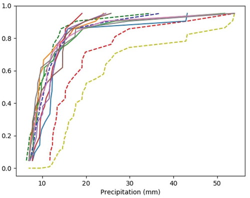
Figure 5. Distributions corresponding to the central four pluviometers and the time aggregation of 15 min. See Figure 3 caption for explanation of lines and units.

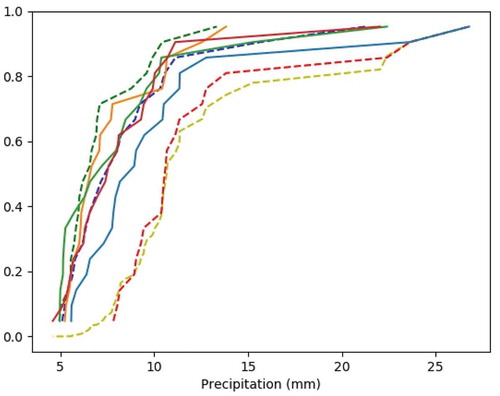
Figure 6. Distributions corresponding to the central eight pluviometers and the time aggregation of 15 min. See Figure 3 caption for explanation of lines and units.

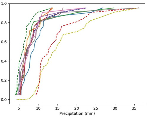
Figure 7. Distributions corresponding to the central four pluviometers and the time aggregation of 3 h. See Figure 3 caption for explanation of lines and units.

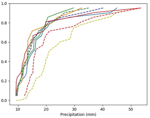
Figure 8. Distributions corresponding to the central eight pluviometers and the time aggregation of 3 h. See Figure 3 caption for explanation of lines and units.

4 Radar fields

The spatial behaviour of extremes may be studied using radar observations. The radar-based extremes, however, often show high errors due to wind drift, signal attenuation and problems with the Z–R relationship (Goudenhoofdt et al. 2017). Bárdossy and Pegram (2017) suggested an indirect method to obtain extremes from radar precipitation. In this paper we use a different approach. The pluviometers described in Section 3 are located about 50 km from the German Weather Service (DWD) radar in Türkheim. The radar images were first corrected for wind drift, and subsequently a non-parametric transformation of the reflectivity to precipitation amounts was performed using the observed pluviometer data as ground truth. The spatial resolution of the radar data is 500 m × 500 m. The method was validated using cross-validation and provided better estimates than a traditional Z–R relationship (Yan and Bardossy 2018). The biggest 47 events of the pluviometer data were considered and the corresponding radar estimations were performed. This number was the count of those large events above a chosen threshold and not sampled at a fixed interval in the 38 months of observation. The extremes show good agreement with the observations.

The “point” extremes (on 500-m square pixels), in a square of 4.5 km × 4.5 km, were calculated. Figure 9 shows the distributions at (1) a fixed point, (2) a point at the maximum precipitation within the area and (3) for the areal precipitation over the nine 1.5-km squares. Note that the distribution of the largest sub-area precipitation exceeds the point precipitation – in other words, it is probable that there is a sub-area where the precipitation will exceed the 1-year point return period amount every year. This sub-area is not always the same, but such a flood event can happen every year in a different part of the area.

Due to the fact that the above observations correspond to a short time period, and that the radar reconstruction is only reliable in the vicinity of the stations, we decided to investigate simulated rainfields.

5 Simulated radar fields

We turn to the determination of the recurrence intervals of extreme rainfall, at fine spatial scale, via the simulation of radar rainfall fields, which were then sampled in appropriate ways.

Outside Bethlehem in South Africa is the site of an S-band radar that was originally used for checking the potential of cloud seeding for rainfall augmentation. This valuable radar rainfall record was the 8-year dataset used to devise and prove the String of Beads Model (SBM, Pegram and Clothier 2001a, 2001b, Clothier and Pegram 2002), which was designed to analyse and simulate 5-min radar scans of rainfall on a 128-km square field. The model was made to mimic the seasonal variation of precipitation in the summer rainfall environment of the high-veld region of South Africa, modelling observed wet durations in addition to variations of intensity and coverage. The rainfields generated in 5-min intervals have varying proportions of dry and rainy areas, where the spatial structure depends on a Gaussian field modified by a spectrum. The Bethlehem radar data are patchy and span only 8 years. Nevertheless, it was shown by Clothier and Pegram (2002) that the spatial structure was relatively well modelled by Gaussian fields. As an alternative we use χ² spatial field dependence, as shown in Section 6 (and Fig. 17), which yields higher local clusters. However, the treatment in this section emphasizes the effect of spatial sampling, which is the main message of this paper. The truncated two-parameter lognormal distribution is fitted to the positive values (>1 mm/h) of each generated image, dependent on the wetted area ratio and the image mean flux. The lognormal is appropriate for modelling extremes, as shown by Papalexiou et al. (2013). For the purposes of this paper, 20 years of 5-min radar rainfall data at 1-km pixel scale were simulated, with seasonality built in, via the SBM. These simulated images had the dry periods replaced by 6-h gaps, as in the gauged data, so we retained “wet” scans to work with. The method of calculating the images is shown schematically in Figure 10 (from Clothier and Pegram 2002, where the methodology is developed in detail).

Figure 9. Configuration of the blocks considered (right). In the left figure the solid (red) line is the distribution of the maxima at the central point. The green dashed line is the distribution of the maxima of the single pixels (81 pixels each 500 m × 500 m) in the 4.5 km × 4.5 km square. The blue dashed line is the distribution of the maxima of the areal means calculated from the amounts in the nine squares (1.5 km × 1.5 km) each. Units are as in Figure 3 caption.

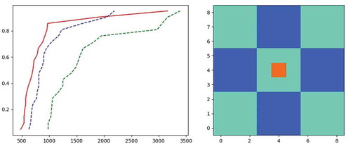
Figure 10. Stack algorithm used to simulate pseudo-random images from image scale statistics, from Clothier and Pegram (2002). WAR: wetted area ratio, IMF: image mean flux.

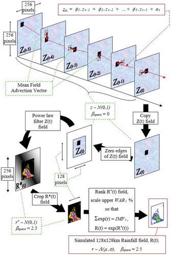
Figure 11. First, third and fifth top-ranked rainfall values of 5-min rainfall over 20 years in 1/10th mm in each 1 km² of 10 000 pixels (Z_L). The colour scale in all three panels ranges from 10 to 26 mm depth. The images in Figures 11–16 were derived from the SBM with Gaussian spatial dependence.

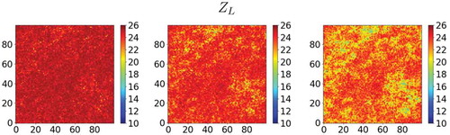
Figure 12. First, third and fifth top-ranked rainfall values of 60-min rainfall over 20 years in 1/10th mm in each 1 km² of 10 000 pixels (Z_L). The colour scale in all three panels ranges from 50 to 270 mm depth.

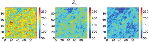
Figure 13. First, third and fifth top-ranked rainfall values of 60-min rainfall in each pixel for the case where we have selected nine pixels centred on the middle one (Z_S). The colour scale in all three panels ranges from 50 to 270 mm depth.

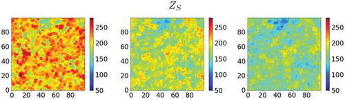
Figure 14. First, third and fifth top-ranked rainfall values of 60-min rainfall in each pixel for the case where we have selected 25 pixels centred on the middle one (Z_S). The colour scale in all three panels ranges from 50 to 270 mm depth.

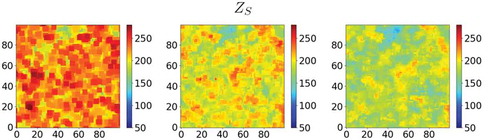
Figure 15. First, third and fifth top-ranked spatially averaged areal rainfall values of 60-min rainfall for the case where we have selected 25 pixels centred on the middle one (Z_A,_D). The maximum intensity of the averaged values is considerably lower than those in Figure 14. The colour scale in all three panels ranges from 50 to 270 mm depth.

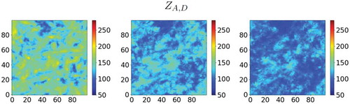
Figure 16. Distributions of extremes. Mauve: average of the single pixel extremes, orange: average of all the mean values over 3 × 3 blocks, blue: average of all the mean values over 5 × 5 blocks, red: average of the maxima over 3 × 3 blocks, and green: average of the maxima over 5 × 5 blocks.

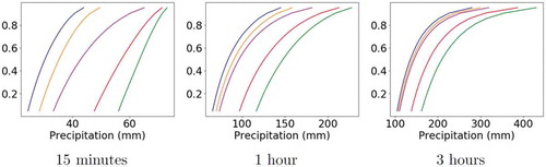
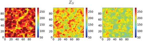
Figure 17. First, third and fifth top-ranked rainfall values (generated using χ² spatial copulas) of 60-min rainfall in each pixel for the case where we have selected 25 pixels centred on the middle one (Z_S). The colour scale in all three panels ranges from 50 to 270 mm depth to compare with Figure 14.

Consider a 20-year stack of about 500 000 “wet” 5-min interval “radar scans” of 128-km square fields, which turns out to be 8.3 × 10⁹ data values to manage as the raw material. The main purpose of this analysis was to determine the frequency of extreme short-term rainfall events in 1-km² pixels averaged successively over areas of 1, 9 and 25 km². In this section of the paper, we do not address ARFs that are used for catchments as a whole, but confine our attention to heavy precipitation occurring somewhere in 1–5-km square areas, not at point locations. The storm durations we treat are 3 h or less, typical durations of severe convective and frontal systems.

The method we chose was to trim the 128 to 100-km squares to avoid edge effects. Each of the 1-km pixels was treated in turn in the following way. Selecting an area, we collect all 5-min rainfall rates on each 1-km pixel over the 20 years and rank the 500 000 wet pixels, in time, from highest to lowest to obtain their sample probability distributions. The next step was to increase the accumulation period from 5 min to 10, 20, 30, 60, 120 and 180 min in turn and obtain these accumulated windows of rainfall blocks in 5-min steps through the record. As mentioned above, the purpose of the 5-min stepping is that we need to capture the highest total in the moving window and not be restricted by non-overlapping intervals of clock time, which we will show reduces the extremes of the sampled rare events. The 10 000 individual series, determined from each centred pixel in the trimmed 100-km square area, are sorted by frequency, and the 20 heaviest amounts over the areas plotted. These sequences represent the “point” values, which might be measured by a large number of individual pluviometers spaced at 1 km and could be interpreted as the conventional intensity or depth duration frequency (IDF or DDF) curves determined from gauges or pluviometers.

In Figure 11 we show a sample of a sequence of the images of the 1-km pixels containing the first, third and fifth ranked rainfall values of 5-min rainfall in each pixel obtained from the sequences of images. The legend bars at the right of each panel show the depth of rainfall in 10ths of millimetres. Note the narrow window of the legend: 10–26 mm.

Staying with the 1-km pixels, the next step is to increase the length of the temporal window from 5 min to 10, 30, 60, 120 and 180 min and examine the behaviour of the rankings. Again, the totals over the lengths of the chosen intervals are calculated from a 5-min moving summing window. In Figure 12 we show the 60-min accumulations at 1-km pixel scale to compare with the 5-min values in Figure 11. Note that the depth scales in Figure 12 are different and cover a wider range: 50–270 mm. Also, note the increased granularity of the images, indicating greater range of variability across the ranked fields.

We next increased the size of the target areas to 3-km square, each centred on the middle point of the square, and found the largest of any one of the nine precipitation values, at each time step, and stored it at the centre pixel site. The thinking here is novel. We want to know what rainfall amount might have happened (and been missed) in pixels surrounding the central pixel (which might be a gauge), and which would threaten local drainage somewhere in the 9-km² area centred on the middle pixel. We are concerned that the “pluviometer” in the centre might have missed the maximum fall in the 3 km × 3 km block, which could do some damage nearby.

Figure 13 shows the three images containing the first, third and fifth ranked rainfall values of the heaviest 60-min rainfall over the full 20 years in each of the nine pixels centred on the middle pixel. The “blockiness” in the first image (not so much in the third and fifth ranked images) in Figure 13 derives from the fact that the heaviest fall on a 1-km pixel in a 3 km × 3 km block dominates, in the sense that as the 3 × 3 mask moves across the field, the largest value will remain the maximum until the mask moves on to a less intense maximum. Again, the scale is in 1/10th mm of precipitation depth. Note that the depth scale is the same as in Figure 12, because the times of accumulation are the same at 60 min.

The above analysis was repeated for a 5 km × 5 km block, which is the largest size we treated, because 25 km² is a relatively large city area and demonstrates our methodology adequately. There follow some examples in Figure 14, where the scale is still 1 km over the 25 km², and the period of accumulation is 60 min. Using the larger blocks to find the maxima led to a further increase of the precipitation amounts. Note that the depth scale is the same as in Figure 12, because the times of accumulation are the same at 60 min.

Comparing the results to the areal averages for 5 km × 5 km blocks one can see that these values from averaging are much lower than the point averages. This is shown in Figure 15, where the depth scale is 50–270 mm, the spatial scale is still 1 km over the 25 km², and the period of accumulation is 60 min. It is evident that the maximum intensity of the averaged values is considerably lower than those in Figure 12.

In Figure 16, we next turn to a different way of summarizing the above results, where panel (a) shows the 2-year cdfs of the mean areal rainfall calculated over all pixels in the 100-km square in the range from 5 to 180 min for different treatments at the 10 000 sites, with the magnitudes of the 20 individual block averages given on the vertical axis in a log scale of 1/10th mm. The left-most (blue) line shows the arithmetic average of the 25 rainfall estimates in the 5 km × 5 km blocks. It lies slightly left of the next (orange) line, which is the arithmetic average of the nine rainfall estimates in the 3 km × 3 km blocks. The middle (mauve) line is the average over the 2 102 400 images of each of the individual single block maximum values at each time step. The fourth (red) line is the average over all the images of the 10 000 3 km × 3 km block maximum values as sampled in Figure 11. The last (green) line is the average of the maximum 9 km × 9 km block values, as sampled in Figure 12. Note the considerable increase of depth of the red and green lines compared to the mauve one. Figure 16(b) is the same as Figure 16(a), except that the values ranked are the 10-year cdfs. Note that the 60-min value of the green line of Figure 16(b) is just below 230 mm, matching the highest value of the first (heaviest rainfall) panel in Figure 12.

In Figure 16(a) and (b), we note that the 3 km × 3 km and 5 km × 5 km areal averages given by the orange and blue lines converge to the mauve line (single cells) as the temporal accumulation increases, as one would expect with an area reduction frequency curve. What is new, and the main message of this paper, is that individual 1-km pixel maxima within the 3 km × 3 km and 5 km × 5 km blocks, as shown in Figure 16(c), are distinctly larger than the estimates from the single 1-km pixels, for a duration of 3 h by factors near 1.3 and 1.5, respectively. The important, surprising and worrying message is that somewhere in a block within a couple of kilometres surrounding a pluviometer there is a patch of ground that is experiencing, on average, much larger short-duration (within 3 h) rainfall depths than are being measured by the gauge.

6 Results of non-Gaussian dependence based radar simulations

The behaviour of the extremes is strongly related to their spatial dependence structure. The SBM simulations of Section 5 were based on a Gaussian spatial dependence, where variograms (or covariance functions) fully describe dependence. However it was shown in Suroso (2017) that spatial rainfall structure (specifically high-intensity events) has asymmetrical dependence with high values showing stronger coherence. In order to quantify the possible effect of these structural differences, the SBM was slightly modified. Instead of transforming the underlying Gaussian field to precipitation, the square of the Gaussian fields was transformed using the same marginal distribution of precipitation. This means that this simulation uses a χ² copula (Bárdossy 2006) as spatial dependence. This copula implies asymmetrical dependence, with a spatial correlation similar to the original model. The consequence of the modified dependence structure is quite strong, specifically for the spatial extremes. As the marginals for this simulation are identical with those of the original SBM model, point extremes are not influenced by this modification of the spatial structure. Thus the extremes shown in Figures 11 and 12 remain the same for this model. In contrast, due to the modification of the spatial structure, the important area-related extremes do change. As an example, Figure 17 shows the 60-min spatial extremes, which are higher than the corresponding SBM ones shown in Figure14. This difference shows how important spatial dependence structure is for the study of the areal aspect of precipitation; it is greater than we thought.

7 Discussion and conclusions

Urban sewer system design is usually based on IDF curves corresponding to single locations. However, these do not reflect the spatial behaviour of precipitation. ARFs reduce the point precipitation for the selected areas. These traditional procedures provide a reasonable design for single sites but do not reflect the area of a considered town. If design is oriented towards return periods of extremes occurring anywhere in the town under consideration, we suggest that design principles require modification.

In this paper, different methods to estimate precipitation extremes of sub-daily resolution were presented. In conclusion:

• Using single station extremes may lead to false conclusions and underestimation in design.

• The larger the area, the more frequently extremes may occur somewhere within that area.

• The spatial dependence structure of precipitation has a major influence on extremes. A strong spatial dependence leads to:

• fewer point extremes within an area, due to many simultaneous occurrences of intense precipitation; and

• higher extremes of spatial averages with a given probability.

  • The maxima of sub-areal precipitation may also exceed the extremes measured at a single point, thus the use of area reduction factors may lead to underestimation of the design.

  • Urban sewer design should consider spatial dependence explicitly, and should not be dependent only on traditional IDFs and ARFs.

Disclosure statement

No potential conflict of interest was reported by the authors.

Additional information

Funding

This work was supported by the Deutsche Forschungsgemeinschaft [BA 1150/18-2].

References

- Aghakouchak, A., Ciach, G., and Habib, E., 2010. Estimation of tail dependence coefficient in rainfall accumulation fields. Advances in Water Resources, 33 (9), 1142–1149. doi:10.1016/j.advwatres.2010.07.003
- Bárdossy, A., 2006. Copula-based geostatistical models for groundwater quality parameters. Water Resources Research, 42 (W11416). doi:10.1029/2005WR004754
- Bárdossy, A. and Pegram, G., 2017. Combination of radar and daily precipitation data to estimate meaningful sub-daily point precipitation extremes. Journal of Hydrology, 544, 397–406. doi:10.1016/j.jhydrol.2016.11.039
- Bell, F., 1976. The areal reduction factor in rainfall frequency estimation. Wallingfor, UK: Institute of Hydrology.
- Bennett, B., et al., 2016. Estimating extreme spatial rainfall intensities. Journal of Hydrologic Engineering, 21, 3. doi:10.1061/(ASCE)HE.1943-5584.0001316
- Burlando, P. and Rosso, R., 1996. Scaling and multiscaling models of depth-duration-frequency curves for storm precipitation. Journal of Hydrology, 187 (1–2), 45–64. doi:10.1016/S0022-1694(96)03086-7
- Chow, V.-T., 1964. Handbook of applied hydrology: a compendium of water-resources technology. New York: McGraw-Hill.
- Clothier, A. and Pegram, G. (2002). Space-time modelling of rainfall using the string of beads model: integration of radar and raingauge data, WRC report No 1010/ 1/02[ISBN 1 86845 835 0], South Africa: Water Research Commission. doi:10.1044/1059-0889(2002/er01)
- Goudenhoofdt, E., Delobbe, L., and Willems, P., 2017. Regional frequency analysis of extreme rainfall in Belgium based on radar estimates. Hydrology and Earth System Sciences, 21 (10), 5385–5399. doi:10.5194/hess-21-5385-2017
- Krajewski, W., Ciach, G., and Habib, E., 2003. An analysis of small-scale rainfall variability in different climatic regimes. Hydrological Sciences Journal, 48, 151–162. doi:10.1623/hysj.48.2.151.44694
- Menabde, M., Seed, A., and Pegram, G., 1999. A simple scaling model for extreme rainfall. Water Resources Research, 35 (1), 335–339. doi:10.1029/1998WR900012
- Papalexiou, S., Koutsoyiannis, D., and Makropoulos, C., 2013. How extreme is extreme? an assessment of daily rainfall distribution tails. Hydrology and Earth System Sciences, 17 (2), 851–862. doi:10.5194/hess-17-851-2013
- Pegram, G. and Clothier, A., 2001a. Downscaling rainfields in space and time, using the string of beads model in time series mode. Hydrology and Earth System Sciences, 5 (2), 175–186. doi:10.5194/hess-5-175-2001
- Pegram, G. and Clothier, A., 2001b. High resolution space-time modelling of rainfall: the “String of Beads” Model. Journal of Hydrology, 241 (1–2), 26–41. doi:10.1016/S0022-1694(00)00373-5
- Serinaldi, F., Bárdossy, A., and Kilsby, C., 2015. Upper tail dependence in rainfall extremes: would we know it if we saw it? Stochastic Environmental Research and Risk Assessment, 29 (4), 1211–1233. doi:10.1007/s00477-014-0946-8
- Simonovic, S., et al., 2016. A web-based tool for the development of intensity duration frequency curves under changing climate. Environmental Modelling and Software, 81, 136–153. doi:10.1016/j.envsoft.2016.03.016
- Sivapalan, M. and Bl¨Oschl, G., 1998. Transformation of point rainfall to areal rainfall: intensity- duration-frequency curves. Journal of Hydrology, 204 (1–4), 150–167. doi:10.1016/S0022-1694(97)00117-0
- Stewart, E., 1989. Areal reduction factors for design storm construction: joint use of rain-gauge and radar data. In: New directions for surface water modelling, proceedings of Baltimore symposium. Wallingford: IAHS Publication No. 181.
- Suroso, 2017. Asymmetric dependence based spatial copula models: empirical investigations and consequences on precipitation fields. Mitteilung ed Vol. Heft 254. Stuttgart University.
- Yan, J. and Bardossy, A., 2018. Non-linear estimation of short time precipitation using weather radar and surface observations. Dresden: Tag der Hydrologie.