A distribution-free ordinal classification of floods based on moments

ABSTRACT

Classification of floods is often based on return periods of their peaks estimated from probability distributions and hence depends on assumptions. The choice of an appropriate distribution function and parameter estimation are often connected with high uncertainties. In addition, limited length of data series and the stochastic characteristic of the occurrence of extreme events add further uncertainty. Here, a distribution-free classification approach is proposed based on statistical moments. By using robust estimators the sampling effects are reduced and time series of different lengths can be analysed together. With a developed optimization procedure, locally and regionally consistent flood categories can be defined. In application, it is shown that the resulting flood categories can be used to assess the spatial extent of extreme floods and their coincidences. Moreover, groups of gauges, where simultaneous events belong to the same classes, are indicators for homogeneous groups of gauges in regionalization.

KEYWORDS:

• flood classification
• Chebychev inequality
• flood coincidence
• regionalization

Editor A. Castellarin Associate editor A. Petroselli

1 Introduction

There are several options to classify observed flood events. A classification of floods is often done with reference to flood types (Viglione et al. 2010), with respect to the return periods of peaks (Hodgkins et al. 2017) or their devastating effects (Ashley and Ashley 2008). Although there exist other criteria of practical relevance (the volume with regard to flood retention or the duration with regard to dikes and infrastructure), the classification of floods by their peak discharge is used in many applications based on flood statistics. Other characteristics are often correlated with flood peaks (e.g. the volume in a type-specific way (Gaal et al. 2012)) or cannot be specified without consideration of the peak (e.g. flood duration). Also, for many practical applications (e.g. estimation of inundated areas) the flood peak is most important, even if flood velocities and duration also determine harmful effects of the floods. To compare simultaneous events in a river basin, the discharges are not suitable. The severity of extreme floods depends on the land use of affected areas and is temporally and spatially variable. That is why the comparability of floods is established by probabilities. Here, exceedence probabilities of the peaks are still dominating flood classifications. For example, in the European Flood Directive (European Commission 2007), measures to reduce flood risk have to be specified for three categories of events: (a) floods with a low probability, or extreme event scenarios; (b) floods with a medium probability; and (c) floods with a high probability (where appropriate). This leads to increased public attention for the classification. Unfortunately, many classification approaches based on probabilities depend on theoretical assumptions such as distribution functions and return periods.

Other classifications of flood events by their types or hydrological circumstances, taking into account e.g. large-scale atmospheric circulation patterns or the atmospheric conditions triggering such an event (e.g. Bárdossy and Filiz 2005, Prudhomme and Genevier 2011), or based on the flood-generating processes (e.g. Gaal et al. 2012), sometimes combined with mathematical procedures such as cluster analysis or decision trees (Sikorska et al. 2015, Turkington et al. 2016), are useful for hydrological and meteorological purposes. Nevertheless, all these approaches demand a deep understanding of the flood-generating processes and are difficult to apply for long time series. Another differentiation between flood events based on peaks over threshold (POT) was proposed by (Merz et al. 2016). The thresholds are derived from the number of occurrences of floods within a time span (1, 3, 5, 10 years, meaning e.g. “on average one event per 10 years”). This approach requires long time series and is affected by the stochasticity of flood series. To classify historic floods between the 14th and 20th centuries, Barriendos et al. (2003) combined hydrological criteria with impact levels (overflow of the usual channels, damages). Barredo (2007) also used damage and loss to estimate the spatial and temporal occurrence of extreme floods in Europe.

In the following, we therefore propose a novel ordinal classification based on the frequency (rarity) of events, similar to that of Merz et al. (2016), but estimation in our method is on the basis of mathematical statistics. Our approach avoids the estimation and explicit utilization of probabilities or return periods. The classification approach proposed here omits any theoretical assumptions such as distributions or estimators, but uses solely empirical distributions and sample characteristics. This not only has the advantage of comparable outcomes but also reduces uncertainty of the estimation procedure. It avoids two problems: first, the flood-statistical evaluation of past extreme flood events is problematic since these events change the distribution parameters and therefore the distribution function. Hence, large differences between estimates before and after the occurrence of such an extreme event could be obtained (see Fischer and Schumann 2016). Moreover, the choice of the theoretical distribution function and the parameter estimation method remains uncertain. Another, more practical advantage is that it is not necessary to perform flood-statistical analyses for all gauges within a river basin after an extreme event. Depending on the applied distribution functions and sample lengths, the results can differ greatly between gauges. These aspects prompted us to propose a much simpler approach based on the Chebyshev inequality that uses only basic statistical characteristics without theoretical assumptions. One disadvantage of the proposed classification is the need to specify subjective thresholds of empirical probabilities. To make the flood characteristics comparable for several gauges, the same thresholds have to be chosen for all gauges in a region. However, the same problem exists if floods are classified by statistical return periods of their peaks. Another problem, which became evident, is related to scales of catchments. For large basins a significant correlation between mode and skewness of the annual maximum series exists, which has to be considered by using the hyper-skewness (fifth moment) instead of the skewness (third moment) to classify flood events by their peaks.

This paper is organized as follows. First, the statistical methodology is explained in Section 2. Then the classification approach is applied on different datasets of annual maximum discharges, in which the scales of watersheds and the spatial extents of the three study regions differ significantly. The results are discussed together in Section 4 to specify the different aspects of the proposed methodology. The last section concludes the results so far.

2 Methods

In the following we propose a method for the classification of floods into different categories. The basis is general statistical characteristics of the flood series, which are extended in a robust way. Moreover, an optimization method is developed to obtain regional consistent classifications.

2.1 Classification

The starting point for the development of a classification for floods is the assumption that the more rarely these events occur, the greater their impact. Rare events are less anticipated, but result in higher water levels, larger flooding and generally more serious consequences. To avoid declarations concerning theoretical probabilities, empirical probabilities of flood peaks have to be translated into qualitative flood classes. Recall that the empirical probability of a flood event with rank m in a sample of length n is given by p = m/(n + 1) (see e.g. Rao and Hamed 2000). One of many possible classifications according to empirical probabilities is given in Table 1. These could be translated directly into empirical return periods T, since T = 1/(1 – p) (Rao and Hamed 2000). In our example, extreme (or very large) floods therefore occur on statistical mean every 30 years, large floods on statistical mean every 15 years, and so on.

Table 1. Possible classification of flood events with probabilities.

Flood class	Qualitative property	Non-exceedence probability p of the peak discharge
1	Small flood	≥ 0.5
2	Medium flood	≥ 0.8
3	Large flood	≥ 0.933
4	Very large flood	≥ 0.966

A classification into four classes is based on the common approach of flood defence measures in Germany, which is based on four flood alert steps. However, the proposed classes are different from the German alert steps, which are fitted to local flood conditions and not connected with probabilities of flood peaks. Their dependencies on flood discharges often vary strongly within a river basin. Of course, the method described in the following can be extended to any number of flood classes.

Mathematically, for a given sample X₁, …, X_n, we need a value k, such that P(X ≥ k) ≤ β, where β is the threshold to be determined. Since this β is mostly based on a chosen probability p, we denote the k calculated with the given p as k_p.

There exist several possibilities to calculate k_p. First of all, one could fit a distribution function and estimate the corresponding quantiles. But, as mentioned above, this leads to a large uncertainty concerning the choice of the distribution and the efficiency of the estimator, especially for small samples. The use of best fit criteria such as AIC and BIC, statistical tests, or model averaging can make the choice less subjective. However, the dependency of the results on the proposed method remains and all three methods do not give an answer on how good the fit is. An empirical estimation of the quantiles is limited to the largest observation of the sample as the largest quantile and therefore for small samples this is also not suitable. This is the reason why we want to estimate k_p based on statistical characteristics such as mean, standard deviation and skewness.

The commonly known inequality for this problem is the Chebyshev inequality. It is applicable for a wide class of probability distributions and specifies the fact that no more than a certain fraction of values can be more than a certain distance away from the mean. This inequality can be sharpened by further assumptions on the random variables that are made because of the hydrological nature of the data. We can assume that the random variables are unimodal. That means that there exists exactly one m such that the distribution function F(x) is convex for x < m and concave for x > m. If the mode is arbitrary, Dharmadhikari and Joag-Dev (1986) generalized a result of Vysochanskij and Petunin (1980) to arbitrary rth moments, r > 0:

(1) $\begin{array}{rl}& \mathrm{P}(\left.|X|\ge k_p\right)\\ & \le max\left\{{\left(\frac{r}{(r+1)k_p}\right)}^r\mathrm{E}{\left|X\right|}^r,\frac{s}{(s-1)k_p^r}\mathrm{E}{\left|X\right|}^r-\frac{1}{s-1}\right\},\end{array}$(1)

where s is a constant, with s > r + 1 and s(s − r − 1)³ = r². For further details on inequalities of this type, we refer to Savage (1961) and Sellke (1996).

In our case, we can restrict ourselves to the first component of the maximum. Due to the calculation of k_p for p ≥ 0.5, it can be shown by simulations that for large p (p > 0.8), the maximum takes exactly this value, and also for smaller probabilities no significant difference occurs for this restriction, but the calculation becomes much easier. This leads us to the case of the so-called generalized Gauss or Camp-Meidell inequality (see e.g. Göb and Lurz 2015), but without the assumed symmetry of the data, which cannot be assumed for flood peaks. The generalized form has the advantage that the additional information used here leads to higher discriminatory power compared to the Chebyshev inequality, which is valid for almost all distributions. This power is increased further in the following.

Since we only have a data sample with unknown moments, we have to estimate these. We are aware that the use of estimates instead of theoretical moments causes an uncertainty that can change the threshold (see Kabán 2012). But these differences are negligible for sufficiently large sample sizes (n ≥ 40). To obtain a sufficient exactness and to take into account the properties of the data such as skewness, we calculate the Camp-Meidell bound with the third moments. The third moments represent the skewness and therefore the heaviness of the tails. This is an important characteristic for many flood series, especially for small and medium catchments, where single extraordinary extreme events occur.

We obtain:

(2) $\mathrm{P}(\left|X\right|\ge k_p)\le {\left(\frac{3}{4}\right)}^3\frac{1}{k_p^3}\mathrm{E}|X{|}^3$(2)

and, since the considered data are discharges and hence positive, the absolute value vanishes. As mentioned above the right hand side of the inequality should equal 1 − p. By transformation to k_p we have:

(3) $k_p=\frac{3}{4}{\left(\frac{\mathrm{E}{(X)}^3}{1-p}\right)}^{\frac{1}{3}}$(3)

Now the non-centred third moment has to be estimated on the basis of the sample x₁, …, x_n with the related order statistic x_(i), i = 1, …, n.

Commonly, the third moment is estimated by the average:

(4) ${\hat{\mu }}_3=\frac{1}{n}\sum _{i=1}^n{x}_i^3$(4)

But this estimator is not robust and therefore not stable over time. The importance of robustness of statistical estimators for hydrological purposes has been emphasized by several authors (e.g. Garavaglia et al. 2011, Kochanek et al. 2014), since it leads to a more stable and often less uncertain estimation. Hence, we use a robust estimator to obtain a time-stable estimation even for small sample sizes. Moreover, a robust estimator increases the discriminatory power of the inequality. Therefore, the mean is replaced by the trimmed mean (see e.g. Huber 2009):

(5) ${\bar{X}}_{\alpha }=\frac{1}{n-2[n\alpha ]}\sum _{i=1+[n\alpha ]}^{n-[n\alpha ]}{x}_{(i)}$(5)

applied to the third power. In detail, 10% of the data (rounded down), that is 5% symmetrically in both the upper and the lower tail, are trimmed. Thus, the calculated thresholds are stable even in the presence of newly occurring extraordinary large or small events. The k_p values are then estimated as follows from the annual maximum discharges:

(6) $k_p=\frac{3}{4}{\left(\frac{\frac{1}{n-2[n\cdot \alpha ]}\sum _{i=1+[n\cdot \alpha ]}^{n-[n\cdot \alpha ]}{x}_{(i)}^3}{1-p}\right)}^{\frac{1}{3}}$(6)

Here, α is the degree of the one-sided trimming, that is α = 0.05.

In case studies it became obvious that for large catchments the use of different moments for the calculation of the thresholds is advisable. We show in the following that many flood series of large catchments are characterized by a combination of a high kurtosis and heavy tails. That is, the medium discharges stay relatively constant whereas single large and small floods occur. This characteristic can be described by the hyper-skewness, which measures the impact of mode and tail-heaviness on the skewness, and equals the fifth moment (Loukeris and Eleftheriadis 2015). Simultaneously with the previous case we derive an estimator for the threshold:

(7) ${\mathrm{k}}_p=\frac{5}{6}{\left(\frac{\frac{1}{n-2[n\alpha ]}\sum _{i=1+[n\alpha ]}^{n-[n\alpha ]}{x}_{(i)}^5}{1-p}\right)}^{\frac{1}{5}}$(7)

A “very large flood” therefore has, for most of the gauges in a region, a peak discharge that is greater than or at least equal to the specific k_0.966 threshold.

It remains to discriminate when to use which moments. As described above, the fifth moments measure the impact of mode and tail on the skewness. High fifth moments refer to a larger impact of the tail, whereas lower fifth moments imply a larger influence of the mode. Since we are interested in extraordinary large floods, the impact of the (right) tail is important. An influence of the mode on the skewness could hence falsify the determination of the threshold if the third moments are used. In this case, the use of the fifth moments is advisable. To determine an objective decision when to use which kind of moment, we want to investigate the explanatory power of the mode for the skewness. This can be done by estimating the correlation between mode and skewness. If the mode has an impact on the skewness, the correlation should be significant. This can be verified by the use of the correlation test (t-test), where we use the Spearman correlation coefficient. This has the advantage of using ranks and hence is robust against single extreme events. Moreover, in contrast to the classical Pearson correlation coefficient it does not assume a linear dependency between both variables.

In the case of a significant correlation between mode and skewness of the annual maximum series, fifth-order moments should be used in the Camp-Meidell inequality.

The probability thresholds chosen in Table 1 can be increased or decreased depending on local flood conditions. The number of exceedences in that case is a very important property for the choice of the thresholds within catchment areas.

2.2 Optimization

To make an objective choice of the probability thresholds possible, we propose an optimization approach. For this, two basic assumptions are made:

• Within a regional group of gauges, the same flood event should be classified in the same way.

• The observed number of exceedences within the time series should be equivalent to the theoretical number.

In this case we call a group of gauges regional if they belong to the same tributary or region. Of course, also other classifications can be used.

Under these assumptions we develop the following optimization criterion:

Suppose we want to determine probability thresholds p₁, …, p_m for m flood classes. If we consider a gauge i, i = 1, …, k, with sample length n_i within a group of gauges, we define $n_{i;p_j}$ as the number of annual maximum discharges of this gauge, whose non-exceedence probability is larger than the threshold p_j and smaller than p_j+1 (i.e. the discharges are larger than k_p and smaller than k_p+1). This threshold should be chosen in such a way that the number of these events in the series of n_i years approximately equals the expected value of the number of events within the class (n_i(1 − p_j) − n_i(1 − p_j+1)); that is, the difference (in absolute value) of both the terms $n_i/n_{i;p_j}$ and n_i(1 − p_j) − n_i(1 − p_j+1) (respectively between $n_i/n_{i;p_m}$ and n_i(1 − p_m) for the largest class) should be minimal. Hence, the optimization criterion is given by the minimum sum of the absolute variation coefficients of the single classes:

(8) $\underset{(p_1,\dots ,p_m|p_1<\dots <p_m)\in \mathbb{N}}{min}\sum _{j=1}^m\left|\mathrm{v}\mathrm{a}\mathrm{r}{C}_{p_j}\right|$(8)

where

(9) $\mathrm{v}\mathrm{a}\mathrm{r}{C}_{p_j}=\left\{\begin{array}{c}\frac{\sqrt{\mathrm{v}\mathrm{a}\mathrm{r}\left(\frac{n_i}{n_{i;p_j}}-\left(n_i(1-p_j)-n_i(1-p_{j+1})\right)\right)}}{\frac{1}{k}\sum _i^k\left(\frac{n_i}{n_{i;p_j}}-\left(n_i(1-p_j)-n_i(1-p_{j+1})\right)\right)}\mathrm{f}\mathrm{o}\mathrm{r}j<m\\ \frac{\sqrt{\mathrm{v}\mathrm{a}\mathrm{r}\left(\frac{n_i}{n_{i;p_m}}-\left(n_i(1-p_m)\right)\right)}}{\frac{1}{k}\sum _i^k\left(\frac{n_i}{n_{i;p_m}}-\left(n_i(1-p_m)\right)\right)}\mathrm{f}\mathrm{o}\mathrm{r}j=m\end{array}\right.$(9)

Here, we use the threshold values defined in Table 1 as starting values.

3 Study area and data

The classification approach is applied to three datasets of annual maximum discharges. The first corresponds to the mesoscale catchment of the Mulde River basin in Saxony, Germany. This basin consists of three sub-catchments, the Freiberger Mulde, the Zwickauer Mulde and, after the point of confluence of both, the United Mulde. Annual maxima are available for 31 gauges with observation periods starting between the years 1910 and 1986. All series end in the year 2013. The catchment size varies from 75 to 6171 km². The Mulde River basin has experienced two extraordinary extreme flood events in recent years, in 2002 and 2013, causing damages of billions of euros. The second dataset consists of gauges located in the eastern Harz region in Saxony-Anhalt, Germany. Here, gauges of several different river basins are considered and all belong to the lower mesoscale. The catchments are very heterogeneous and differ significantly in their elevations, flow directions, land use and orographic conditions. The catchment sizes for this dataset are between 3.4 and 456 km². A detailed overview of the land use and catchment size of both datasets is given in Table A1 in the Appendix.

The third dataset includes gauges in the whole of Germany and is based on the GRDC (Global Runoff Data Centre) database. Here, annual maxima of 44 gauges with a catchment area of at least 10 000 km² are considered, which refer to large catchments. The gauges belong to the five main rivers in Germany (Rhine, Main, Danube, Elbe and Weser) and their tributaries.

4 Application

Before applying the classification approach, it has to be determined which moment order should be used for the basins. To obtain consistent results, and since the catchments are of similar size within one basin, the moment order is chosen consistently within a basin.

The results of estimated Spearman correlation coefficients (ρ) between mode and skewness for the different basins are given in Table 2. It becomes obvious that the correlation between mode and skewness for the macroscale catchments is significantly higher. For each of the catchments, the correlation deviates significantly from zero, which would imply independence. It can be seen that the correlation coefficient between mode and skewness seems to increase with increasing catchment size. The Elbe, Danube, Rhine, Main and Weser basins, all of which contain only catchments of at least 10 000km², have a much higher correlation than the mesoscale catchments.

Table 2. Spearman’s correlation coefficient, ρ between mode and skewness for the different river basins considered in the datasets.

River basin/region	Correlation coefficient, ρ
Harz	0.1351
Zwickauer Mulde/United Mulde	0.0462
Freiberger Mulde	–0.1188
Elbe	0.4666
Danube	0.4047
Rhine	0.5002
Main	0.6324
Weser	0.4047

Application of the correlation test shows that the hypothesis of independence of mode and skewness cannot be rejected for the Harz region and both Mulde basins. Since the partial samples of the main rivers of the macroscale dataset are rather small (n ≈ 10) the application of a test statistic does not deliver reliable results. There exist tables of critical values for small samples, but it is also known that the test has less power for these sample sizes. Hence, we decided to combine annual maxima of the main rivers into one dataset, where the discharges are normalized by the median, to make a comparison possible. The correlation coefficients described above are rather similar and, hence, a combination is sensible. For this combined dataset the hypothesis of independence between mode and skewness is rejected. Consequently, for the macroscale catchments it is not sensible to use the third moments since the skewness is greatly influenced by the mode.

The hypothesis of increasing correlation between mode and skewness for increasing catchment size is analysed for the Inn basin. The Inn is a tributary of the Danube and has the advantage that it consists of gauges of size 3.64–28 357 km² and thus includes meso- and macroscale sub-basins. Since the gauges belong to the same basin, they are comparable. The dataset is available online (www.gkd.bayern.de). For all 69 gauges in the dataset the mode and skewness are estimated. Then the correlation coefficient between both characteristics is calculated by the Spearman correlation coefficient, where the data sample is extended in each step by the next largest catchment. The starting dataset consists of the smallest 20 catchments, with a size smaller than 32 km² to avoid uncertainty in the estimation. This procedure makes it possible to determine a possible change in correlation according to the catchment size. All time series are checked for possible trends using the Mann-Kendall test, where no significant trend was found, and robustness is obtained by the use of the Spearman correlation. The results are presented in Figure 1. A distinct change in the correlation can be observed when catchments of 1000 km² and larger are added to the sample. A stable correlation is then obtained again at a catchment size of about 6000 km²; it should be noted that there are no gauges with catchment areas between 1200 and 6000 km². The correlation of about 0.1 for small catchments corresponds with the results for the other mesoscale catchments of the Mulde and Harz datasets. However, the correlation never reaches the size of the macroscale catchments, as we have the large impact of the mesoscale catchments in the dataset.

Figure 1. Correlation between mode and skewness for 69 gauges in the Inn River basin.

Based on the results of the correlation test and the analysis of the Inn catchment, we decided to use third moments for the mesoscale catchments up to 6171 km² and fifth moments for the macroscale catchments. If the Inn dataset is considered, the dataset should be split into meso- and macroscale catchments.

After defining the moment order, the probability thresholds have to be determined. This is done with the optimization method proposed above using simulated annealing and minimizing the variation coefficient given in Section 2 applied to each basin. As starting values, the empirical probabilities in Table 1 are used. The resulting thresholds are given in Table 3. For the large catchments, all thresholds are compared between all river basins. Hence, the thresholds should be chosen consistently. For these cases, we decide to use the starting values given in Table 1 as thresholds. These are close to most of the optimized thresholds.

Table 3. Resulting probability thresholds after applying optimization to the datasets for the Mulde basin and Harz region.

	Probability threshold
River basin	Class 1 (small floods)	Class 2 (medium floods)	Class 3 (large floods)	Class 4 (very large floods)
Harz	0.5	0.875	0.928	0.973
Freiberger Mulde	0.5	0.875	0.916	0.952
Zwickauer Mulde/United Mulde	0.875	0.916	0.944	0.971

The classification results for selected years for the two mesoscale datasets Harz and Mulde are given in Figures 2–4. The observed annual maximum discharges are coloured according to their flood class. For readability, only selected years are given in the illustrations. The given beginning and end of the annual maximum series indicate that all but three discharge series have at least 40 years of observations. We decided to include three series of less than 40 years to show that the approach is nevertheless applicable, although these results have a higher uncertainty. Additionally, the estimated limits of the flood classes (k_p) are given. The gauges are sorted according to their location in the river basin, which can be seen by the gauge IDs. The different colours describe the classification of the annual maxima according to the flood classes of the different events. A detailed analysis of distinct events concerning their extent and generation is given in Section 5.

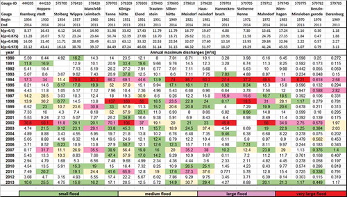
Figure 2. Flood classification for the annual maximum discharges of the gauges in the sub-catchment Freiberger Mulde. The annual maximum discharges are coloured according to their flood class.

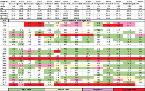
Figure 3. Flood classification for the annual maximum discharges of the gauges in the sub-catchment Zwickauer Mulde/United Mulde. The annual maximum discharges are coloured according to their flood class.

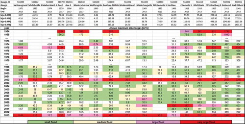
Figure 4. Flood classification for the annual maximum discharges of the gauges in the Harz region. The annual maximum discharges are coloured according to their flood class.

As mentioned above, the number of events within one flood class is linked directly with the empirical probability. In fact, the number of events exceeding one threshold should equal approximately 1 – 1/p. The ability to reach this by the optimization is shown in Figure 5, where for the optimized p = 0.875 approximately eight annual maximum events are above the threshold, which is equal to T = 1 – 1/p.

Figure 5. Number of annual maximum discharges above the optimized threshold k_0.875 for all gauges in the Harz region. The empirical return period is highlighted as a solid line.

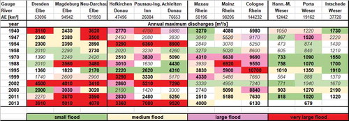
For the macroscale catchments, results are only presented for selected years and gauges to ensure readability (Fig. 6). For such large catchments and different main rivers the problem occurs that not every annual maximum at every gauge belongs to the same event. Hence, we define an annual maximum as belonging to the same event when the dates of the peaks differ by less than 6 days. The main annual maximum then is chosen according to the date of the event with the highest flood classification and is highlighted in the illustration.

Figure 6. Flood classification of annual maximum series for selected years and gauges of the macroscale dataset, with the main flood shown in bold and all remaining flood events being shaded.

5 Discussion

It has been shown that macroscale catchments have a much higher correlation between mode and skewness than mesoscale catchments. This means their skewness is much more influenced by the mode instead of heavy tails. Since the mode defines the value that occurs most, a large correlation between mode and skewness implies a large amount of values of the same size, in this case medium floods. As we consider the flood peaks only as a random variable, we argue that this is caused to a certain degree by discharges overtopping the banks and the resulting retention of flood waves, which reduce the increase of peaks with low exceedence probabilities downstream.

However, such extreme floods in large basins require a much extended rainfall event where many tributaries are affected nearly simultaneously by an extreme flood. This is rather rare and, hence, for most floods the hydrographs will be smoothed downstream within large basins.

If a mesoscale basin is only partially affected by a flood, for example caused by heavy rain, the hydrograph is less smoothed because of the fast reaction. Hence, an extreme flood in part of the basin will also be classified as an extreme flood at a gauge downstream. This leads to heavy tails of the flood series.

A comparison of two gauges, which are located very far downstream in their respective basins, is given in Figure 7. The two gauges Wechselburg/Zwickauer Mulde (2107 km²) and Cologne/Rhine (144 232 km²) are compared in a histogram. The very different nature, especially of the tails, becomes obvious. Moreover, the annual maximum series of Cologne has a more pronounced mode.

Figure 7. Histogram for the annual maximum floods of the gauges Wechselburg/Zwickauer Mulde (left) and Cologne/Rhine (right).

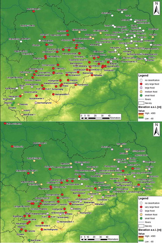
Application of the classification approach shows that the large floods (magenta) and very large floods (red) especially are classified alike for neighbouring gauges for the Mulde River basin (Figs 2 and 3). The two extraordinary extreme events in 2002 and 2013 clearly stand out in the classification and are classified as large and very large floods, respectively, for all gauges but one. The spatial extent of the flood events can be seen in Figure 8, where gauges in the whole of Saxony are considered. Whereas the event in 2002 occurred in the whole Mulde River basin with very large peaks, the event of 2013 does not have such extreme peaks in the southern parts of the basin. Instead, often the coincidence of the events of two tributaries may increase the flood classification to “very large”, even if the gauges upstream do not measure peaks of this category. This corresponds with the rainfall events that lead to such flood events. In 2002, heavy convective rain led to hydrographs with high peak and small volume, whereas the event in 2013 was caused by long-duration rainfall on moist soil. Hence, only parts of the Elbe River were affected and very large floods only occurred locally, as can be seen when the considered area is extended to the whole of Saxony (Fig. 8, bottom).

Figure 8. Extent and classification of the flood events in 2002 (top) and 2013 (bottom) in the upstream tributaries of the Elbe River in Saxony, Germany.

Another extreme event is detected at the Freiberger Mulde in 1975. In this year, parts of the Mulde River basin were affected by long-lasting rainfall during December 1974, resulting in large floods. The flood event in 2010 is only classified as a large or very large event for the gauges downstream of the Zwickauer Mulde, since only parts of the catchment were affected by the rain event.

Moreover, events in 1954 (Zwickauer Mulde) and 1958 (Freiberger Mulde) are classified as very large and large, respectively. This corresponds to the flood behaviour for these years. In 1954, extraordinary long and heavy rainfall, especially in the area of the Ore Mountains, affected mainly the sub-catchment Zwickauer Mulde and led to large floods, for example in the area of Zwickau. In 1958, the centroid of the heavy rainfall was located near Dresden and thus the eastern part of the Mulde, and therefore the sub-catchment Freiberger Mulde was much more affected. In addition to these special events, behavioural similarities of small clusters of gauges can be detected. The gauges Streckewalde and Hopfgarten, as well as Berthelsdorf, Nossen and Niederstriegis, show very similar behaviour for several years. These gauges are located very close together and their topographical similarity leads to this similar behaviour. Although the catchments are very heterogeneous in terms of land use, the proposed method makes the annual maximum discharges comparable, which would not be possible if only the observed flood peaks were used instead of a classification. Even catchments with a high urbanization such as Chemnitz can be compared to other catchments with less urbanization concerning the magnitude of a flood peak.

In the Harz region, the event in 2002 was one of the largest flood events in this area too. It was only exceeded by the event in 1994. In this year, the Vb weather condition, which is very unusual in this region, led to unusually heavy and long rainfall in an area at the lee side of the Brocken Mountain. Both events are classified here as extreme large events for many gauges (Fig. 4). Since the Harz basin consists of many different river systems that are not necessarily connected, it is not unexpected that the gauges show different classifications for the same event.

For the macroscale catchments in the German dataset, spatial coherence is rare. It can be seen that certain very large flood events only occur at single main rivers (Fig. 6).

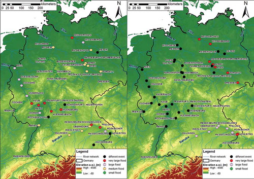
To investigate this further, two distinct events are considered according to their spatial distribution in Germany: the events in the years 1988 and 2002 (Fig. 9). It becomes obvious that the event in August 2002 was the only annual maximum flood event for the Elbe and Danube gauges, where it is classified as large and very large (Fig. 9, right). It can be seen that, for all western gauges (Rhine and Weser) in Germany, the annual maximum discharges occurred at another time. In 1958, there was no common annual maximum at all. But also floods can be observed that affected the whole of Germany in all main rivers. In 1995, the event that is classified as very large for the Rhine catchments is also observed as an annual maximum for all other catchments. A rather global flood event was the event of March/April 1988, which occurred in all five main rivers and is classified as very large for gauges in four of the main river basins (Fig. 9, left).

Figure 9. Classification of the flood events of 1988 (left) and 2002 (right) for the gauges considered in the macroscale dataset.

If the dates of these events are compared, it becomes clear that most of the events that affected more than one of the main rivers occurred in the winter months (November–April), although in recent years more and more summer floods have occurred for many catchments. This can probably be explained by the snowmelt, which affects many main rivers at the same time, although this has decreased in recent years because of higher temperatures and hence less snow.

6 Conclusions

A flood classification method is applied to three datasets of meso- and macroscale catchments. The proposed classification method is based solely on statistical characteristics of the observed discharges and does not assume any distribution. Moreover, by the use of robust estimation methods it is more stable over time and not affected by single extraordinary small or large events. The thresholds for the flood classes are obtained by an extension of the classical Chebyshev inequality, the Camp-Meidell inequality, and moments of certain order are applied. We propose two different moment orders, third and fifth moments. It is shown that the moment order depends greatly on the catchment size and that macroscale catchments need a higher moment order due to their dominating mode.

The results of classification into four flood classes give an indication of the magnitude of the floods. The direct linkage to empirical probabilities makes a comparison with classical applications in water management possible. The results are consistent within the mesoscale datasets, and coherence between gauges can be detected. It is also possible to classify the spatial extent of a flood event by comparing the classifications within a basin.

For macroscale catchments the coherence is no longer so obvious, since the use of annual maximum discharges can lead to floods belonging to different events that are not comparable. Nevertheless, many events occur in two or more main rivers at the same time and a few events also affect catchments in the whole of Germany. The results show that winter floods in general seem to have a larger spatial extent than summer floods.

Since the method is applicable to any resolution of data, further studies should compare summer and winter annual maxima and monthly maxima of discharge to consider the different spatial extents of winter and summer floods. Moreover, it will be used for the classification of certain flood types to investigate possible dependencies between flood type and flood class.

The classification results can be used not only to make spatial extent visible, but also to form the basis for a regionalization approach, where they can be used for the definition of homogeneous groups of gauges. Although applicable to all regions, regardless of homogeneity, homogeneous groups will lead to clusters of events that are equally classified and hence the proposed method can be used as a measure of homogeneity.

Acknowledgements

The authors would like to thank Bayerisches Landesamt für Umwelt (LfU Bayern), Sächsisches Landesamt für Umwelt, Landwirtschaft und Geologie (LFULG), Landesbetrieb für Hochwasserschutz und Wasserwirtschaft (LHW) Sachsen-Anhalt and The Global Runoff Data Centre (56068 Koblenz, Germany) for providing the data.

Disclosure statement

No potential conflict of interest was reported by the authors.

Additional information

Funding

The financial support of the German Research Foundation (“Deutsche Forschungsgemeinschaft”, DFG) in terms of the research group FOR 2416 “Space-Time Dynamics of Extreme Floods (SPATE)” is gratefully acknowledged.

Appendix

Table A1. Overview of the catchment sizes and land use for the Mulde and Harz datasets, sorted according to flow direction.

		Land use (%)
Catchment/River	Area (km^2)	Urban	Agriculture	Grassland	Forest	Water bodies
Sachsengrund/Zwickauer Mulde	6.47	0.00	0.00	0.00	100.00	0.00
Schönheide 3/Zwickauer Mulde	149.00	4.13	1.13	7.28	86.65	0.81
Markersbach 1/Gr. Mittweida	30.07	0.38	2.67	2.29	94.66	0.00
Aue 1/Schwarzwasser	363.00	7.18	6.10	18.78	67.73	0.21
Aue 3/Schwarzwasser	682.00	6.47	4.45	14.86	73.50	0.73
Niederschlema/Zwickauer Mulde	754.00	7.98	6.36	15.36	69.64	0.66
Wolfersgrün/Crinitzer Wasser	21.65	3.13	59.38	13.02	24.48	0.00
Zwickau-Pölbitz/Zw. Mulde	1021.00	11.04	17.40	15.93	55.15	0.48
Niedermülsen 1/Mülsenbach	49.57	7.89	57.00	15.27	19.85	0.00
Niederlungwitz/Lungwitzbach	138.00	17.14	53.14	17.59	12.12	0.00
Altchemnitz 1/Zwönitz	144.00	12.37	36.74	15.21	35.68	0.00
Harthau/Würschnitz	136.00	15.35	52.64	14.46	17.55	0.00
Chemnitz 1/Chemnitz	403.00	24.80	40.98	11.93	22.29	0.00
Göritzhain/Chemnitz	532.00	23.73	45.21	11.79	19.27	0.00
Wechselburg 1/Zwickauer Mulde	2099.00	15.24	35.17	13.57	35.77	0.26
Golzern 1/United Mulde	5433.00	10.29	40.76	17.10	31.58	0.26
Bad Düben 1/United Mulde	6170.00	9.76	43.64	15.91	30.38	0.30
Tannenberg/Zschopau	91.50	5.54	16.23	37.07	41.16	0.00
Wiesa/Pöhlbach	86.44	7.79	17.58	37.32	37.32	0.00
Streckewalde/Pressnitz	206.00	1.90	8.06	25.02	63.52	1.51
Hopfgarten/Zschopau	530.00	6.06	14.56	32.04	46.71	0.63
Rothenthal/Natzschung	75.94	0.70	1.93	14.24	83.13	0.00
Zöblitz/Schw. Pockau	125.00	6.28	11.67	21.48	60.57	0.00
Borstendorf/Flöha	640.00	4.41	15.72	21.94	57.51	0.42
Lichtenwalde/Zschopau	1572.00	6.50	23.22	24.97	44.93	0.38
Kriebstein UP/Zschopau	1754.00	6.91	27.08	23.91	41.68	0.41
Wolfsgrund/Freiberger Mulde	35.84	4.59	49.18	30.82	15.41	0.00
Berthelsdorf/Freiberger Mulde	245.00	4.46	40.42	27.53	26.90	0.69
Nossen 1/Freiberger Mulde	586.00	8.00	53.14	18.84	19.73	0.29
Niederstriegis 1/Gr. Striegis	286.00	7.04	65.71	13.81	13.44	0.00
Erlln/Freiberger Mulde	2980.00	7.28	41.55	20.17	30.71	0.30
Ilsenburg/Ilse	21.4	0.00	0.00	0.30	96.40	0.00
Hoppenstedt/Ilse	160	6.90	57.00	2.10	33.30	0.20
Stolberg/Thyra	31.7	0.60	2.00	0.20	97.20	0.00
Wippra/Wipper	136	2.60	39.60	2.80	54.70	0.20
Mansfeld-Leimbach/Wipper	210	3.00	43.70	1.70	51.60	0.10
Tanne/Warme Bode	71.5	3.00	5.20	0.00	91.10	0.10
Königshütte WB/Warme Bode	100	2.30	6.20	1.30	89.70	0.00
Elend/Kalte Bode	25.7	3.90	0.10	1.20	89.60	0.20
Trautenstein/Rappbode	39.1	3.40	11.90	10.80	74.10	0.00
Silberhütte/Selke	105	2.60	31.30	5.30	60.90	0.00
Meisdorf/Selke	184	2.50	22.40	3.10	71.90	0.00
Hausneindorf/Selke	456	5.50	53.70	1.30	36.30	0.00
Hanneckenbruch/Holtemme	9.4	0.00	0.00	0.00	100.00	0.00
Steinerne Renne/Holtemme	15.7	0.70	0.00	0.00	99.30	0.00
Mahndorf/Holtemme	168	8.00	45.30	0.70	45.90	0.00
Nienhagen/Holtemme	270.5	8.60	59.70	1.20	30.30	0.10
Minsleben/Barrenbach	13.7	21.20	67.20	7.50	4.20	0.00
Benzingerode/Hellbach	3.4	5.30	60.90	0.00	33.90	0.00
Derenburg/Hellbach	26.7	1.70	5.20	0.00	93.10	0.00

References

- Ashley, S.T. and Ashley, W.S., 2008. The storm morphology of deadly flooding events in the United States. International Journal Climatology, 28 (4), 493–503. doi:10.1002/(ISSN)1097-0088
- Bárdossy, A. and Filiz, F., 2005. Identification of flood producing atmospheric circulation patterns. Journal of Hydrology, 313, 48–57. doi:10.1016/j.jhydrol.2005.02.006
- Barredo, J.I., 2007. Major flood disasters in Europe. 1950–2005. Natural Hazards, 42 (1), 125–148. doi:10.1007/s11069-006-9065-2
- Barriendos, M., et al., 2003. Stationarity analysis of historical flood series in France and Spain (14th–20th centuries). Natural Hazards and Earth System Sciences, 3, 10.
- Dharmadhikari, S. and Joag-Dev, K., 1986. The Gauss–tchebyshev inequality for unimodal distributions. Theory of Probability & Its Applications, 30 (4), 867–871. doi:10.1137/1130111
- European Commission, 2007. Directive 2007/60/EC of the European parliament and of the council of 23 October 2007 on the assessment and management of flood risks. Available from: http://ec.europa.eu/environment/water/flood_risk/index.htm [Accessed 15 Apr 2018].
- Fischer, S. and Schumann, A., 2016. Robust flood statistics: comparison of peak over threshold approaches based on monthly maxima and TL-moments. Hydrological Sciences Journal, 61 (3), 457–470. doi:10.1080/02626667.2015.1054391
- Gaal, L., et al., 2012. Flood timescales: understanding the interplay of climate and catchment processes through comparative hydrology. Water Resources Research, 48. doi:10.1029/2011WR011509
- Garavaglia, F., et al., 2011. Reliability and robustness of rainfall compound distribution model based on weather pattern sub-sampling. Hydrology and Earth System Sciences, 15 (2), 519–532. doi:10.5194/hess-15-519-2011
- Göb, R. and Lurz, K., 2015. The use of inequalities of camp-meidell type in nonparametric statistical process monitoring. In: S. Knoth and W. Schmid, eds. Frontiers in statistical quality control Vol. 11. Basel, Switzerland: Springer International Publishing, 163–182.
- Hodgkins, G.A., et al., 2017. Climate-driven variability in the occurrence of major floods across North America and Europe. Journal of Hydrology, 552, 704–717. doi:10.1016/j.jhydrol.2017.07.027
- Huber, P.J., 2009. Robust statistics. New Jersey, USA: John Wiley and Sons.
- Kabán, A., 2012. Non-parametric detection of meaningless distances in high dimensional data. Statistics and Computing, 22 (2), 375–385. doi:10.1007/s11222-011-9229-0
- Kochanek, K., et al., 2014. A data-based comparison of flood frequency analysis methods used in France. Natural Hazards and Earth System Science, 14 (2), 295–308. doi:10.5194/nhess-14-295-2014
- Loukeris, N. and Eleftheriadis, I., 2015. Further higher moments in portfolio selection and A priori detection of bankruptcy, under multi‐layer perceptron neural networks, hybrid neuro‐genetic MLPs, and the voted perceptron. International Journal of Finance and Economics, 20, 341–361. doi:10.1002/ijfe.1521
- Merz, B., Nguyen, V.D., and Vorogushyn, S., 2016. Temporal clustering of floods in Germany: do flood-rich and flood-poor periods exist? Journal of Hydrology, 541 (Part B), 824–838. doi:10.1016/j.jhydrol.2016.07.041
- Prudhomme, C. and Genevier, M., 2011. Can atmospheric circulation be linked to flooding in Europe? Hydrological Processes, 25, 1180–1190. doi:10.1002/hyp.v25.7
- Rao, A.R. and Hamed, K.H., 2000. Flood frequency analysis. Boca Raton, USA: CRC Press.
- Savage, I.R., 1961. Probability inequalities of the Tchebycheff type. Journal of Research of the National Bureau of Standards-B. Mathematics and Mathematical Physics B, 65, 211–222.
- Sellke, T., 1996. Generalized Gauss-Chebyshev inequalities for unimodal distributions. Metrika, 43 (1), 107–121. doi:10.1007/BF02613901
- Sikorska, A.E., Viviroli, D., and Seibert, J., 2015. Flood-type classification in mountainous catchments using crisp and fuzzy decision trees. Water Resources Research, 51, 7959–7976. doi:10.1002/2015WR017326
- Turkington, T., et al., 2016. A new flood type classification method for use in climate change impact studies. Weather and Climate Extremes, 14, 1–16. doi:10.1016/j.wace.2016.10.001
- Viglione, A., et al., 2010. Quantifying space-time dynamics of flood event types. Journal of Hydrology, 394 (1–2), 213–229. doi:10.1016/j.jhydrol.2010.05.041
- Vysochanskij, D.F. and Petunin, Y., 1980. Proof of the 3 σ rule for unimodal distributions. Theory of Probability and Mathematical Statistics, 21, 25–36.