A probabilistic framework for floodplain mapping using hydrological modeling and unsteady hydraulic modeling

ABSTRACT

Prediction of design hydrographs is key in floodplain mapping using hydraulic models, which are either steady state or unsteady. The former, which require only an input peak, substantially overestimate the volume of water entering the floodplain compared to the more realistic dynamic case simulated by the unsteady models that require the full hydrograph. Past efforts to account for the uncertainty of boundary conditions using unsteady hydraulic modeling have been based largely on a joint flood frequency–shape analysis, with only a very limited number of studies using hydrological modeling to produce the design hydrographs. This study therefore presents a generic probabilistic framework that couples a hydrological model with an unsteady hydraulic model to estimate the uncertainty of flood characteristics. The framework is demonstrated on the Swannanoa River watershed in North Carolina, USA. Given its flexibility, the framework can be applied to study other sources of uncertainty in other hydrological models and watersheds.

KEYWORDS:

• floodplain mapping
• hydrological modeling
• unsteady hydraulic modeling
• uncertainty analysis

Editor R. Woods Associate editor H. Kreibich

1 Introduction

Reliable flood risk assessment, estimation of insurance rates and planning for mitigation measures require detailed spatio-temporal information about flood characteristics such as depth and velocity. Given the rarity of extreme flooding, hydraulic models are typically applied to derive these flood characteristics and produce floodplain hazard maps. Since these models are prone to uncertainties, the predicted flood characteristics (e.g. depth and velocity) will themselves be uncertain. Overlooking the uncertainty of predicted flood characteristics has major influences on predicted inundation (Bales and Wagner 2009, Di Baldassarre et al. 2010). This can result in underestimated or overestimated flood risk (Kalyanapu et al. 2012) and incomplete representation of the effectiveness of flood mitigation measures, thereby leading to the selection of sub-optimal alternatives during the decision-making process (Meyer et al. 2009).

Uncertainty in flood modeling arises from the input variables, choice of performance measures to test the model efficiency, and calibration/validation data as well as uncertainties over the model structure and parameters (Krzysztofowicz and Kelly 2000, Krzysztofowicz and Herr 2001, Pappenberger et al. 2006, Liu and Gupta 2007, Smemoe et al. 2007, Di Baldassarre and Montarari 2009, McMillan et al. 2010, Aronica et al. 2012b, Saint-Geours et al. 2014). A particular area of concern is how to incorporate the uncertainty of design hydrographs in floodplain mapping, which can be the most influential factor in inundation modeling (Schaffenberg and Kavvas 2011, Savage et al. 2016b, Bermúdez et al. 2017). When a steady state hydraulic model is applied, a peak discharge is required for input, while a full hydrograph is required as the upstream boundary condition for an unsteady simulation. Previous research using steady state simulation has applied a peak discharge estimated from flood frequency analysis (e.g. Smemoe et al. 2007). Steady state simulation, which is the common practice for floodplain mapping in the USA, only provides information on an envelope of flood depth and extent and is unable to provide any information about flood wave dynamics. Steady state models also tend to overestimate flood depths and extent because the floodplain is assumed to fill instantaneously compared to the more realistic dynamic case (Neal et al. 2013, Ruiz-Bellet et al. 2017).

Unsteady hydraulic models therefore provide a fuller picture of flood dynamics by predicting detailed information on time-variant flood characteristics. Past uncertainty analysis efforts via unsteady models have been based largely on a joint flood frequency–shape analysis, with only a very limited number of studies using ensembles of hydrological models to provide uncertain hydraulic model boundary conditions (e.g. Pappenberger et al. 2005, Bermúdez et al. 2017, Breinl et al. 2017). However, those studies that have used hydrological models to provide boundary conditions in this way have not done so with the intention of creating design hydrographs. Instead, studies that have produced unsteady design hydrographs have derived either a single hydrograph attribute, peak (e.g. Kalyanapu et al. 2012, Aronica et al. 2012b, Neal et al. 2013), or two attributes, peak and volume (Aronica et al. 2012a, Candela and Aronica 2017), through a flood frequency analysis and later fitted a synthetic time series to these attributes (shape analysis). This approach requires making additional assumptions and may increase the flow computation error (Morris et al. 2009). A shape analysis to obtain the full hydrograph is somewhat arbitrary (Aronica et al. 2012b) and ignores different timings of the contributing flow sources as an additional source of uncertainty (Neal et al. 2013). In addition, a single attribute or combination of multiple attributes can provide a limited description of plausible flood events (Ahmadisharaf et al. 2018). Another limitation of this approach is the need for a long set of observed flow data, which is not always available (Rogger et al. 2012). In watersheds where future changes in land use (e.g. urbanization) and stream condition (e.g. levee construction) are expected, a flood frequency analysis is often not a reliable approach to estimate design floods (Viglione et al. 2009). Another limitation of this approach is that it is not spatially explicit and is only applicable to particular geographical points where a streamgauge is available. Application of a hydrological model to transform design rainfall to derive the complete design hydrograph may be less subjective, paving the way for an automated floodplain mapping through coupling hydrological and hydraulic models.

One concern about using ensembles of hydrological models to derive the upstream boundary condition of the hydraulic models is the high computational cost needed by hydraulic models to route numerous hydrographs through the downstream areas (Vacondio et al. 2014). In particular, application of multidimensional unsteady hydraulic models for probabilistic analysis is expensive and requires computationally efficient models that are still not widely available (Alfonso et al. 2016, Teng et al. 2017). However, recent advances in the computational capabilities of hydraulic models, e.g. JFLOW-GPU by Lamb et al. (2009), Flood2D-GPU by Kalyanapu et al. (2011), and RiverFlow2D GPU by Hydronia LLC (2016), can assist floodplain managers in efficiently using probabilistic analyses. Considering these advances in unsteady simulation, ensembles of hydrological models can be utilized to predict hydrographs, which can then be coupled with hydraulic models for probabilistic inundation modeling. Coupled hydrological and hydraulic modeling provides a comprehensive representation of flood wave routing over the simulation boundary by accounting for the backwater effects of the floodplains in damping and delaying flows (Bravo et al. 2012).

A further limitation in floodplain mapping practice, which is caused by employing steady state models, is that the uncertainty is often reported for maximum flood depth and extent without spatially quantifying the uncertainty of other risk-influencing characteristics that vary over time. Although these other characteristics are correlated to flood depth, detailed information on them may be crucial for reliable risk estimation and rational decision making (Dang et al. 2011, Qi and Altinakar 2011a, 2011b, 2012, Ahmadisharaf et al. 2015). In particular, floodplain mapping efforts (Romanowicz and Beven 2003, Bates et al. 2004, Quinn et al. 2013, Buahin et al. 2017, Faghih et al. 2017, Papaioannou et al. 2017) have been rather limited to maximum inundation extent, wherein the floodplain boundary was determined as a flood probability map, a more reliable alternative to a single definitive inundation extent. Despite limited efforts (e.g. Aronica et al. 2012b, Savage et al. 2016b), the uncertainty of other flood characteristics has not been studied extensively.

The overarching objective of this paper is therefore to develop a generic probabilistic framework to derive the uncertainty of flood characteristics – extent, depth, velocity, duration, arrival time and time of maximum inundation – by coupling a hydrological model with a two-dimensional (2D) unsteady hydraulic model. Two uncertainty sources – design rainfall depth and antecedent moisture condition (AMC) – are considered to demonstrate the probabilistic framework. These sources are exemplars to illustrate the framework, and the extension to consider a fuller range of uncertainty sources is relatively trivial due to versatility of the presented scheme. Through application of an unsteady hydraulic model, we also seek to investigate whether the temporal variation of the uncertainty of flood characteristics is negligible. The framework is illustrated for the rainfall-driven overbank flooding event that took place on the Swannanoa River watershed in the state of North Carolina, USA.

2 Methodology

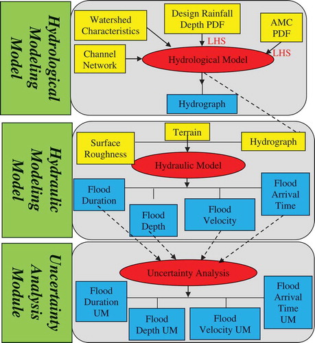
The research objective is achieved by developing a probabilistic framework for spatial uncertainty analysis of flood characteristics (Fig. 1). The framework utilizes three modules: a hydrological model to generate an ensemble of hydrographs, an unsteady hydraulic model for inundation modeling, and an uncertainty analysis tool to estimate the uncertainty of flood characteristics on a cell-by-cell basis. These models are linked, such that outputs from the hydrological model feed into the hydraulic model and the outputs (flood characteristics) of the latter feed into the geospatial uncertainty analysis tool. Latin hypercube sampling (LHS; McKay et al. 1979) is applied to propagate the uncertainty of hydrological model inputs (rainfall depth and AMC herein) to the output hydrographs. Using an ensemble of hydrographs in the hydraulic model results in an ensemble of flood characteristics – depth, velocity, duration, arrival time and time of maximum inundation – that are later processed via the uncertainty analysis tool and are characterized through empirical cumulative distribution functions (ecdf) in each grid cell. The ultimate deliverable of the developed framework is a map showing the uncertainty of each flood characteristic. The remainder of the Methodology section, which discusses the framework modules in detail, is organized as follows. An overall picture of the hydrological model, including primary inputs, uncertain variables, simulation of overland flow, channel routing and uncertainty propagation method to predict stochastic design hydrographs, is given in Section ‎2.1. Inundation modeling using the 2D unsteady hydraulic model is described in Section ‎2.2. The proposed approach to perform the spatial uncertainty analysis is discussed in Section ‎2.3.

Figure 1. Schematic of the probabilistic framework for spatial uncertainty analysis of flood characteristics. LHS: Latin hypercube sampling; AMC: antecedent moisture condition; pdf: probability density function; UM: uncertainty map.

2.1 Hydrological modeling module

A semi-distributed hydrological model, which was developed in the GoldSim® environment (GoldSim Technology Group 2017), was applied here to simulate hydrological processes. GoldSim® is a dynamic simulation software with applications ranging from water resources management to financial predictions, and provides a versatile user-friendly graphical user interface for probabilistic modeling. The model divides the entire watershed into a number of sub-watersheds that are interconnected by river reaches. Rainfall time series in tandem with the characteristics of river cross-sections (e.g. geometry, bed slope and Manning’s roughness) and sub-watersheds (e.g. area, hydrologic soil group and land use) are taken as model inputs and hydrographs are generated at the outlets of sub-watersheds and on the river reaches. To simulate rainfall–runoff process, the Snyder’s unit hydrograph (Snyder 1938) and the Natural Resources Conservation Service (NRCS) curve number (CN; NRCS 1986) are used as the transform and rainfall excess methods, respectively. In application of the NRCS method, the ratio of potential maximum retention to initial abstraction is set to 0.05 as suggested by Woodward et al. (2003).

While the use of the NRCS method for sub-daily simulations has been questioned by some researchers (e.g. Garen and Moore 2005, Grimaldi et al. 2013b, Grimaldi and Petroselli 2015), past successful applications have showed its efficiency even for sub-daily time steps (e.g. Grimaldi et al. 2013a). In addition, as discussed by Grimaldi et al. (2013a), application of the NRCS method for sub-daily simulations does not affect the findings of a comparative analysis, as is the case in our probabilistic application. The Muskingum channel routing method of the US Army Corps of Engineers (USACE 1936) is employed to route flow through the streams. A rainfall time series can be assigned to each sub-watershed. Groundwater processes are not taken into account in this model. The developed hydrological model does not compute the baseflow, but takes the baseflow data calculated from the Web-based Hydrograph Analysis Tool (WHAT; Lim et al. 2005).

To employ the hydrological model in the probabilistic framework, a probability density function (pdf) was assigned to the uncertain variables. We focused on the uncertainty of the design hydrograph, induced by two inputs of the hydrological models – rainfall depth and AMC – both of which have a substantial impact on the predicted hydrograph (Singh 1997, Merwade et al. 2008) and flood characteristics (Smemoe et al. 2007, Aronica et al. 2012b). In particular, many researchers have found AMC to be the most influential parameter in hydrograph prediction (among others, De Michele and Salvadori 2002) even in severe storms (Marchi et al. 2010). Thus, the uncertainty of both variables needs to be incorporated for reliable floodplain mapping. We acknowledge the presence of other uncertainties (e.g. model structure) in hydrological modeling, but a comprehensive uncertainty analysis would make a clear demonstration of the framework more difficult. Selection of these two important drivers in an effort to illustrate our proposed framework and extension to other uncertainties should be a relatively trivial step. However, a sensitivity analysis (Section ‎2.1.1) was done to show the importance of the two selected uncertain variables in the hydrological model.

A uniform pdf was assigned to the design rainfall depth since it does not assume any prior knowledge about parameter uncertainty (Beven and Binley 1992). To demonstrate the uncertainty attributed to the AMC, three classes, dry (AMC I), normal (AMC II) and wet (AMC III) (NRCS 1986) are taken into account. A discrete pdf is used to perturb the uncertainty of AMC in line with previous research (e.g. De Michele and Salvadori 2002), with each AMC class is assumed to have a probability of 0.33.

The LHS with random points in strata was applied for uncertainty propagation using the GoldSim® built-in Monte Carlo simulation toolbox (GoldSim Technology Group 2017). This is an efficient sampling method (Helton and Davis 2003) and is commonly preferred to the standard Monte Carlo method because a smaller sample size is required for numerical convergence (Melching 1995, Hall et al. 2005, Janssen 2013). At each LHS realization, the hydrological model generated a hydrograph, resulting in an ensemble of hydrographs. Each of these hydrographs was fed into the hydraulic modeling module. The model was validated for the Swannanoa River watershed by Ahmadisharaf (2016) against the Hurricane Ivan flood event in September 2004. Multiple goodness-of-fit measures, including the Nash-Sutcliffe efficiency criterion (NSE; Nash and Sutcliffe 1970), percent bias (PBIAS), coefficient of determination (R²), index of agreement (d) (Willmot 1984) and root mean square error (RMSE), were used to test the model efficiency. The validation suggests that the model satisfactorily predicts the streamflow, with NSE of 0.56, PBIAS of −25.4%, R² of 61.4%, d of 0.86 and RMSE of 1.26 m³/s (based on the criteria recommended by Moriasi et al. 2015). The hydrological model was also successfully applied in watershed-scale hydrological modeling by Ahmadisharaf et al. (2015, 2016). Additional details on the hydrological model can be found in Ahmadisharaf (2016). In addition to the validation against this historical event, the simulated peak magnitudes for eight 24-h design storms – 2-, 5-, 10-, 25-, 50-, 100-, 200- and 500-year storms – were compared with flood frequency results of a streamgauge at the Swannanoa watershed outlet (Weaver et al. 2009). We found that the simulated range of peak values (5th–9th) in all these eight events fell inside the 90% prediction interval.

2.1.1 Sensitivity analysis of the hydrological model

A sensitivity analysis was conducted to evaluate the importance of the two selected uncertain variables on the outputs of the hydrological model. A dimensionless sensitivity index, the elasticity index (EI; Loucks et al. 2005), was used to measure the sensitivity of the hydrograph attributes – peak, time to peak, and volume – with respect to the model input and parameters. A greater EI suggests a higher level of sensitivity. Our goal was to justify that both rainfall depth and AMC are relevant and important in hydrograph simulation compared to other sources of uncertainty in the hydrological model such as model parameters. Alongside the rainfall depth and AMC, we tested multiple model parameters, including Snyder’s unit hydrograph (storage coefficient, ratio of base time to time to peak and lag time) and Muskingum channel routing parameters (Manning’s coefficient of the channels and celerity weight). The results of this analysis for the 100-year design storm showed that the peak discharge is mostly influenced by rainfall depth (EI = 1.47), but the ratio of base time to time to peak in the Snyder’s unit hydrograph is more influential for time to peak and hydrograph volume (EI = 1.08 and 20.79, respectively). While rainfall depth does not affect time to peak (EI = 0.00), AMC has a minor influence on it (EI = 0.02). Aside from this hydrograph attribute, peak and volume are more influenced by rainfall depth (EI = 1.47 and 1.40, respectively) than AMC (EI = 0.48 and 0.47, respectively). This analysis revealed that the selected uncertain variables are of importance for prediction of the hydrograph attributes, but the impact of other potential uncertain parameters should be borne in mind.

2.2 Hydraulic modeling module

The hydraulic modeling module uses a 2D unsteady hydrodynamic model named Flood2D-GPU (Kalyanapu et al. 2011). Developed in NVIDIA’s CUDA programming environment, it is a physically-based model that solves the linear hyperbolic Saint Venant equations using a first-order accurate upwind difference scheme to generate flood depths and velocities (Kalyanapu et al. 2011). The equations are developed from the Navier-Stokes equations by integrating the momentum and continuity equations over the flow depth. To discretize the governing 2D shallow water equations, an upwind finite difference numerical scheme is employed since it yields non-oscillatory solutions through the careful inclusion of numerical diffusion. A staggered rectangular grid stencil is used to define the computational boundary, with horizontal/vertical velocities on the edges of the grid cell and water depth in the grid cell center. The Courant-Friedrichs-Lewy condition is used to constrain the future model time step.

Despite the advantages of 2D hydraulic models over one-dimensional (1D) models, such as better topographic representation, more accurate simulation of flow paths and consideration of lateral interactions between channel and floodplain (Horritt and Bates 2002, Qi and Altinakar 2012, Jung and Merwade 2015), high computational cost often hinders their application for probabilistic analysis in practical applications (Teng et al. 2017). The Flood2D-GPU model takes advantage of a graphics processing unit (GPU) and provides a significantly reduced computational time (by a factor of 80–88) compared to CPU-based models (Kalyanapu et al. 2011). It is thus advantageous for probabilistic analyses where high computational cost is expected. The model was validated against the Taum Sauk Dam breach flood event using the F^<2> statistic (Bates and De Roo 2000), as well as overestimation and underestimation of the inundation extent (Kalyanapu et al. 2011). This validation revealed the excellent performance by the model with F^<2> 75.1 and 15.3% overestimation and 13.1% underestimation of the flood extent. Additionally, Flood2D-GPU was successfully applied in simulation of riverine (Kalyanapu et al. 2012, 2015, Yigzaw et al. 2013, Ahmadisharaf et al. 2015, 2016) and dam-break flooding (Kalyanapu et al. 2011, Ahmadisharaf et al. 2013).

Required datasets for the Flood2D-GPU model are: (i) a DEM for terrain representation; (ii) Manning’s roughness; and (iii) the hydrograph at the source location as the upstream boundary condition. The downstream boundary condition is Neumann (free flow condition), in which the gradient at the outlet is equal to zero. The velocity of the adjacent upstream cells is equated. Raw outputs include the flow depth and velocity at different time steps during the simulation. These results were post-processed to derive the maps of maximum flood depth and velocity as well as flood duration, arrival time and time of maximum inundation (corresponding time of maximum flood depth) using a geospatial toolbox within ArcGIS™ and a series of MATLAB scripts. A threshold of 0.67 m was considered in the computation of arrival time (USACE 2015a).

While Flood2D-GPU is a computationally efficient physically-based model for inundation modeling, the following limitations should be taken into account: (i) lateral flows downstream of the source location cannot be incorporated, which is likely not a serious issue in simulation of large flood events; (ii) the surface roughness of the entire computational domain is uniformly characterized with Manning’s coefficient (Hunter et al. 2007); and (iii) the disadvantage of using the Neumann condition is that the downstream boundary condition is less constrained than a stage condition, but it does not have a significant impact since the free flow boundary is moved downstream for the computational domain. This also avoids the need to predict upstream inflow and downstream stage in a consistent way, as noted by Bermúdez et al. (2017). Ongoing research attempts to address the above-mentioned limitations.

2.3 Uncertainty analysis module

A modified format of the measure proposed by Jin et al. (2010) was used to estimate the uncertainty of the flood characteristics. The modified measure is called the relative interval length (RIL) and is computed as a function of the lower and upper limits, as well as the median of a given hydraulic model output. The original measure by Jin et al. (2010) was called the “average RIL” and was proposed for calibration of probabilistic hydrological models. The RIL is a normalized measure, and provides a comparative uncertainty band for flood characteristics with various units and is computed through the following equation:

(1)

where x_L and x_U are the lower and upper percentiles, respectively; and is the median value. The greater the RIL, the more the uncertainty and vice versa. Taking the lower and upper quartiles as x_L and x_U yields the widely used measure of the ratio of interquartile range (IQR) to the median. Here, the 5th and 95th percentiles are used as the lower and upper limits, in line with many previous inundation modeling studies (among others, Pappenberger et al. 2005, Jung and Merwade 2012). A similar measure has been used by many researchers (e.g. Castro-Bolinaga and Diplas 2014) to quantify the uncertainty of inundation maps.

To perform the geospatial uncertainty analysis, Equation (1) was applied to quantify the uncertainty of flood characteristics in each grid cell. A MATLAB script was implemented to conduct the geospatial uncertainty estimation and ArcGIS was used to visualize the maps.

2.3.1 Comparative analysis of the uncertainty of flood characteristics

For comparative analysis of the uncertainty, we divided flood characteristics based on their spatial and temporal variation (Table 1). The characteristics were divided into two main groups with respect to the spatial variation: (a) space-variant: those that vary with geographic location, including flood depth, velocity, duration, arrival time and time of maximum inundation; and (b) spatially lumped: those that represent an overall characteristic of the entire area of interest, including maximum flood extent as well as average maximum depth and velocity. The latter two were calculated by taking the spatial mean of depth and velocity in the flooded grid cells in each random sample. From a temporal perspective, the characteristics were divided into two groups: (i) time-variant: those that vary over time, including flood depth, velocity and extent; and (ii) temporally lumped: these represent an overall flood behavior over time or take a single value over the simulation period. These characteristics include duration, arrival time and time of maximum inundation. Since the hydraulic model runs with a dynamic time step (see Section ‎2.2), we did not perform a detailed temporal analysis on a time step basis, but rather investigated the temporal mean (over the simulation time) of the time-variant characteristics (temporal mean of extent, depth and velocity) and the difference with temporal maximum. A comparison between the temporal mean and maximum magnitudes of the time-variant characteristics provides a measure of the time dependency of the uncertainty. The least and most uncertain characteristics were identified in both the spatial and the temporal analysis. In all these comparative analyses, only the flooded cells were included. Through these experiments, the importance of spatial and temporal dimensions in uncertainty analysis of floodplain maps was investigated. Subsequently, the importance of spatial uncertainty analysis and unsteady hydraulic models was explored.

Table 1. Variation of the flood characteristics with space and time.

Characteristic	Space	Time
Flood extent	Spatially lumped	Time variant
Flood depth	Space variant	Time variant
Flood velocity	Space variant	Time variant
Flood duration	Space variant	Temporally lumped
Flood arrival time	Space variant	Temporally lumped
Time of maximum inundation	Space variant	Temporally lumped

3 Case study

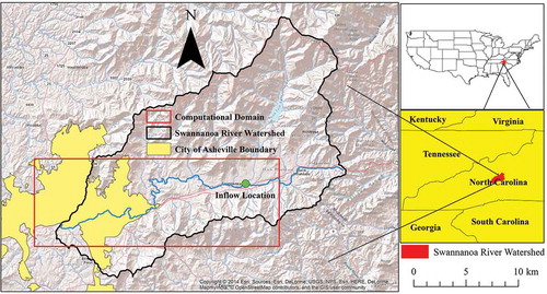
The probabilistic framework was demonstrated using the Swannanoa River watershed located in Buncombe County, North Carolina, USA (Fig. 2). The watershed, which is a part of the larger French Broad River basin, is located in the western North Carolina Mountains, from Asheville to Montreat. The area was selected due to its proximity to the southeastern coast of the USA, which exposes it to the potential path of flood-causing hurricanes and tropical storms. There are developed areas in the watershed, with the City of Asheville being the most urbanized area. The watershed is non-tidal and overbank flooding occurs regularly in the watershed. Land cover is predominantly forest. The average ground slope is 20.9% within the selected computational domain and 21.4% in the floodplains (some areas have a slope of greater than 45%), implying a hilly case. Time of concentration of the watershed was estimated as 17.3 h (City of Asheville 2006). The area has experienced several harmful floods in the past, including the 1916, 1928, 1940, 1964, 1977 and 2004 events. The most severe flooding occurred in 2004 during hurricanes Frances and Ivan and resulted in damage to infrastructure of US$54 million, 11 fatalities and significant disruption to the communities in the watershed (USACE 2015b). While there are warning systems in the watershed, no certified flood control reservoir or levee is located in the region. The 33.3-km Swannanoa River reach, which is bounded by an area of 343.9 km² upstream of its confluence with French Broad River, was selected for this study. The 100-year (1% annual exceedence probability) rainfall-driven overbank flooding was analyzed. In the USA (and many other countries), this recurrence interval is the standard design event (base flood) used by the Federal Emergency Management Agency (FEMA) to develop flood insurance rate maps (FIRMs). One US Geological Survey (USGS) streamgauge, Biltmore (USGS #03451000), which has been operated since 1985, is located in the watershed outlet. Lack of an upstream streamgauge did not allow for development of an upstream design hydrograph through a flood frequency analysis. Therefore, hydrological modeling was needed to derive the design hydrograph. Two National Oceanic and Atmospheric Administration (NOAA) raingauges located in the watershed were used in hydrological modeling.

Figure 2. Watershed location along with the computational domain and inflow location for hydraulic modeling.

4 Results

4.1 Hydrological modeling

For hydrological modeling, the watershed was delineated into 35 sub-watersheds, consistent with the hydrological model development presented in the watershed report by the City of Asheville (2006), and the initial parameters of the sub-watersheds (e.g. CN, lag time and Manning’s roughness of the channels) were taken from the same report. Among these parameters, the ratio of base time to time to peak and storage coefficient in the Snyder’s unit hydrograph, as well as CN, were selected as calibration parameters based on the model sensitivity found by Ahmadisharaf (2016). The sensitivity was quantified via the EI. The nearest gauging approach was used to account for the spatial heterogeneity of rainfall depth, wherein Swannanoa (#318448) represents the upstream areas (20 sub-watersheds) and Asheville (#310301) does so for the downstream areas (15 sub-watersheds). The deterministic hydrological model was calibrated by Ahmadisharaf (2016) against three flood events measured at the study watershed outlet. The model was found to satisfactorily predict the streamflow (Moriasi et al. 2015), with NSE > 0.77, |PBIAS| < 18.7%, R² > 76.8%, d > 0.93 and RMSE < 0.59 m³/s. As discussed in Section ‎2.1, the model validation was judged to be satisfactory. The reader is referred to Ahmadisharaf (2016) for additional details on model calibration and validation in the study area.

In implementation of the hydrological model ensemble, the lower/upper confidence bounds and deterministic values for the 24-h, 100-year design event were taken from NOAA Atlas 14.2 (Bonnin et al. 2006) and were used as the minimum and maximum of the uniform pdf (RIL = 0.16) of the rainfall depth. NRCS Type II was chosen as the temporal rainfall pattern according to the NRCS (1986) suggestions for the study region. It is a dimensionless 24-h rainfall distribution that was originally developed using the National Weather Service duration–frequency data and additional local storm data. To avoid the generation of unrealistic storm events, correlation between the storm depth and AMC was analyzed. A poor correlation was found (Pearson’s correlation coefficient < 0.04) and, therefore, no correlation was used to relate these two variables in the LHS application. One hundred realizations of LHS were settled. To ensure that the number of LHS realizations is adequate, the ecdfs of the hydrograph attributes and estimated uncertainty bands were then compared with those from 1000 realizations. The analysis confirmed that the generated hydrographs are not significantly different (less than 0.4% variation in the uncertainty of maximum peak, time to peak and volume) when the number of realizations increases. Therefore, the framework application proceeded with 100 LHS realizations.

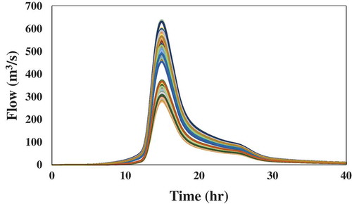
For hydrological modeling of the design event, only the 139.6-km² drainage area of the inflow location (see Fig. 2) was simulated on a 10-min time step. The 100 generated hydrographs were identically shaped because the selected uncertain variables (rainfall depth and AMC) do not substantially affect the timing attributes of the hydrograph (see also Section ‎2.1.1) which are rather sensitive to variables such as surface roughness and watershed slope (McCuen 2009); these were not considered uncertain in this paper, which is methodological in focus. The simulated peak at the inflow location of the hydraulic model (see Fig. 2) ranged from 278.4 to 637.9 m³/s (RIL = 0.64). The predicted 5th–95th range closely matched the 90% prediction interval of the 100-year peak magnitude through USGS regionalized regression equations (Weaver et al. 2009), with both lower and upper bounds being slightly overestimated (279.5 vs 285.6 m³/s and 614.5 vs 627.2 m³/s). The time to peak has a slight variation from 14.9 to 15.0 h (RIL = 0.02), while the hydrograph volume ranges from 7.1 × 10⁶ to 1.5 × 10⁷ m³ (RIL = 0.60). The ensemble hydrographs were used as inputs in the hydraulic model (Fig. 3).

Figure 3. 100-year design hydrographs at inflow location (upstream boundary of hydraulic model).

4.2 Hydraulic modeling

The deterministic hydraulic model was calibrated by Ahmadisharaf et al. (2015) against the August 1994 flood event using peak discharge and travel time accuracy measures (Schubert and Sanders 2012). A peak discharge of 164.8 m³/s was recorded on 17 August at 14:00 h in the Biltmore station located in the watershed downstream. The calibration of Flood2D-GPU suggested an optimal Manning’s value of 0.05 (spatially uniform for the entire computational domain). With this Manning’s value, the model satisfactorily simulated the peak and time to peak with 0.8 and 12.8% absolute error, respectively. The reader is referred to Ahmadisharaf et al. (2015) for additional details on model calibration. The USGS National Elevation Dataset digital elevation model (DEM) (https://nationalmap.gov/elevation.html) with a spatial resolution of 30 m was used based on the general recommendations by Savage et al. (2016a) for probabilistic inundation modeling and Ahmadisharaf et al. (2013) for Flood2D-GPU application in the study watershed. To ensure the DEM appropriately represents the channel geometry, we estimated the cross-sectional area error at multiple cross-sections on the main river. Our investigation revealed that the DEM has an average channel cross-sectional area error smaller than 5.3% and was judged to satisfactorily represent the channel cross-sections. A threshold depth of 0.1 m was used to distinguish between unflooded (dry) and flooded (wet) grid cells following previous flood modeling applications (e.g. Aronica et al. 2002, Savage et al. 2016b) and the DEM vertical accuracy (Gesch et al. 2014). The hydrographs from the hydrological model were used as the upstream boundary condition.

The calibrated hydraulic model was applied to the 100-year design flood of the Swannanoa River watershed for the ensemble of hydrographs. Each ensemble member had a hydrograph duration of 120 h and the number of computational cells was approximately 200 000. Running the model for the 100 realization ensemble took about three days on a computer with two Intel Xeon DP Six Core X5690 3.46-GHz Processors, 32-GB RAM, and one PNY NVIDIA Quadro™ FX5800 graphics card with 240 CUDA streaming processors. The same simulation on a CPU-based model would require about 80 times longer (approximate estimation by Kalyanapu et al. 2011). Running the model resulted in 100 inundation maps. An ensemble of flood extent (maximum and temporal mean); depth (maximum, average maximum and temporal mean); velocity (maximum, average maximum and temporal mean); duration; arrival time; and time of maximum inundation was generated subsequently. The predicted 100-year peak discharge at Biltmore station fell inside the range estimated through frequency analysis by Weaver et al. (2009).

4.3 Uncertainty analysis of flood characteristics

4.3.1 Spatially lumped flood characteristics

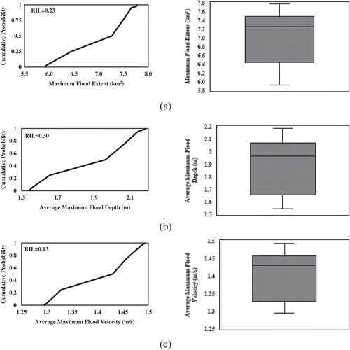
The ecdf of the maximum flood extent as well as average maximum depth and velocity are presented alongside the box-and-whisker plot in Figure 4. Using Equation (1), RIL values of 0.23, 0.30 and 0.13 were computed for the maximum flood extent and average maximum depth and velocity, respectively, suggesting that, of the three spatially lumped characteristics, velocity is the least uncertain and depth is the most. The uncertainty of average maximum depth and maximum extent is close, and both were nearly two times wider than the uncertainty of rainfall depth. All of the spatially lumped flood characteristics were less uncertain than peak and volume of the hydrograph.

Figure 4. Empirical cumulative distribution of the spatially lumped flood characteristics: (a) maximum extent, (b) average maximum depth, and (c) average maximum velocity. RIL: Relative interval length.

4.3.2 Space-variant flood characteristics

The ecdf of the space-variant flood characteristics (depth, velocity, duration, arrival time and time of maximum inundation) was constructed in each grid cell and corresponding RILs were calculated via Equation (1). An uncertainty map was developed for each characteristic (Fig. 5). The smallest spatial range of RIL was 0.04–0.72 and belonged to arrival time, while velocity showed the widest range (0.00–5.12). Arrival time also had the lowest spatial mean RIL (0.13), while depth had the highest (0.64). The overall greater uncertainty of depth can be attributed to the selected uncertain inputs, rainfall depth and AMC, which mostly affect the peak and volume of the hydrograph, but not the shape. Consequently, the time-dependent flood characteristics were less affected.

Figure 5. Uncertainty map of the space-variant flood characteristics: (a) maximum depth, (b) maximum velocity, (c) duration, (d) arrival time, and (e) time of maximum inundation. RIL: Relative interval length.

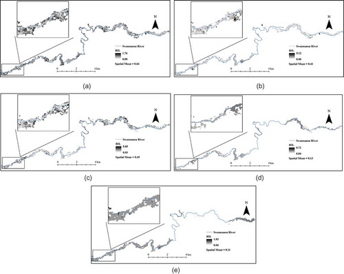
A cell-by-cell analysis of the uncertainty maps was also performed to investigate how the spatial mean of RIL is compared to its values in the inundation area. In 45.4, 42.1, 42.4, 64.3 and 57.3% of the inundation area, the uncertainty of flood depth, velocity, duration and arrival time, and time of maximum inundation was greater than their corresponding spatially averaged uncertainty. These numbers suggest that using a spatially lumped value to represent the uncertainty (taking an average) can be misleading, and the spatial dimension needs to be incorporated for uncertainty analysis of floodplain mapping. For flood depth and velocity, this can be further observed by comparing the spatial mean of the uncertainty of maximum flood depth and velocity (Fig. 4) against the uncertainty of their average maximum (Fig. 3).

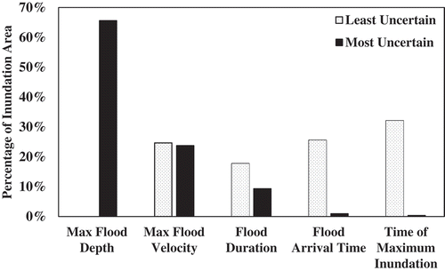
The uncertainty of the five space-variant flood characteristics was compared spatially to identify the least (minimum RIL) and most (maximum RIL) uncertain flood characteristic in each grid cell. The results of this comparative analysis are given in Figure 6. Flood depth was the most uncertain characteristic in more than 65% of the inundation area, while the duration, arrival time and time of maximum inundation had the highest uncertainty in less than 11% of the inundation area. These three were the least uncertain characteristics in more than 75% (accumulative) of the grid cells, with time of maximum inundation being the least uncertain in 32.1% of the study watershed. On the other hand, flood depth was not the least uncertain in any of the grid cells. These findings underline the fact that hydrological model predictions on hydrograph timing attributes (e.g. time to peak) are not very sensitive to the two uncertain variables (design rainfall depth and AMC), but these two substantially affect the peak and volume (see Sections ‎2.1.1 and ‎4.1). Subsequently, the time-dependent flood characteristics were influenced less, while the two others (depth and velocity) were affected more. It can also be noticed that although depth was the most uncertain characteristic in a majority of the study watershed, the other four space-variant characteristics were the most uncertain in nearly one-third of the watershed. Therefore, a single uncertainty analysis of maximum flood depth cannot provide a detailed picture of the uncertainty of floodplain maps, and more attention should be paid to other space-variant flood characteristics.

Figure 6. Percentage of the inundation area for which each space-variant flood characteristic is least/most uncertain.

4.3.3 Time-variant flood characteristics

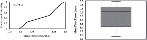
The ecdf of the mean flood extent is presented alongside the box-and-whisker plot in Figure 7. An RIL of 0.17 was computed through Equation (1), which was close to the uncertainty of rainfall depth, but about four times less uncertain than peak and volume of the hydrograph. The uncertainty of mean flood extent was about two-thirds smaller than its maximum, suggesting that the uncertainty varies over the simulation time.

Figure 7. Empirical cumulative distribution of the temporal mean flood extent. RIL: Relative interval length.

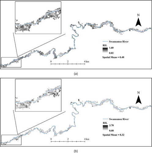
The uncertainty map of the temporal mean flood depth and velocity is given in Figure 8. Similar to the maximum flood depth, which was found to be the most uncertain space-variant characteristic in a major portion of the study watershed, mean depth was also the most uncertain characteristic in 80.1% of the inundation area. Maximum depth and velocity were more uncertain than their mean in 90.0 and 66.7% of the inundation area. The uncertainty of mean depth and velocity can be much smaller than their maximum by up to 160 and 39 times. However, mean depth and velocity can be much more uncertain than their maximum by factors of up to six and 51. The substantial variation of the uncertainty over the simulation time suggests that the uncertainty is rather dynamic, implying that steady state models cannot capture the whole picture of uncertainty and, therefore, detailed unsteady hydraulic simulations are needed for floodplain mapping.

Figure 8. Uncertainty map of the time-variant flood characteristics: (a) mean depth and (b) mean velocity. RIL: Relative interval length.

5 Discussion and conclusions

The uncertainty of flood characteristics was evaluated using the developed probabilistic framework. Our comparative analysis on the uncertainty of flood characteristics revealed that, overall, flood depth has the widest uncertainty, while time-dependent characteristics (duration, arrival time and time of maximum inundation) have the tightest uncertainty, primarily because the selected uncertainties (rainfall depth and AMC) do not substantially affect temporal attributes of the hydrograph. However, it was found that the least and most uncertain characteristics substantially vary with space and time. This finding concerning the temporal variation of the uncertainty corroborates the findings of a previous study by Aronica et al. (2012b). Savage et al. (2016b) also found that the sensitivity of the predicted flood characteristics with respect to the inputs varies both temporally and spatially. We showed that using spatially or temporally lumped frameworks to present the uncertainty can misrepresent the uncertainty of flood characteristics. Therefore, it is recommended that the space and time dimensions be incorporated into uncertainty analysis studies of floodplain mapping by employing spatio-temporal frameworks and detailed unsteady hydraulic models. Our results are, however, strictly valid only for a single case study and subject to our assumptions and limitations, as discussed in detail in the forthcoming paragraphs.

The findings on the relative uncertainty of flood characteristics show the sole contribution of the selected uncertain inputs (rainfall depth and AMC). Other uncertain inputs such as channel and watershed characteristics, which can affect the hydrograph timing (McCuen 2009) and, in turn, the time-variant flood characteristics (Nuswantoro et al. 2016), were not taken into account. Even in terms of rainfall depth, only a large storm (100-year event) and a single duration (24-h) was studied. We expect that other storm severities and durations might result in a different uncertainty of flood characteristics (Bezak et al. 2018). The uncertainty pertaining to the spatio-temporal variability of rainfall was also not investigated, both of which can affect the inundation modeling results (Merwade et al. 2008). We therefore suggest that our findings should be cautiously replicated to other flood events and watersheds. A more comprehensive analysis should be performed to draw more generalized conclusions by cascading all the uncertainty sources. However, in the presence of many uncertainty sources, such a study requires enormous amounts of time and cost, especially via multidimensional unsteady hydraulic models.

Additionally, only a single case study was used to investigate the uncertainty of the design rainfall depth and AMC on flood characteristics as a result of a rainfall-driven overbank flooding. The study watershed in this research was mostly hilly (average ground slope of 20.9% in the computational domain), where floods are often deep and flashy, and do not last long. Such deep, rapid and short-lived flooding implies high depth, fast velocity and arrival time, as well as short duration and time of maximum inundation. The derived uncertainty bands for the flood characteristics are expected to vary in a flat watershed, where floods are likely shallow, slow moving and long duration. Additionally, the study area was mostly rural, where surface roughness is relatively high. The estimated uncertainty of the flood characteristics would likely vary in an urbanized watershed. An analysis of other watersheds was beyond the scope of this paper, which focused on a spatio-temporal comparative analysis of flood characteristics as a result of rainfall depth and AMC. However, our framework is generic and applies not only within the watershed, but also in any other flood-prone areas. Focusing on a single case allows certain conclusions to be drawn. Additional cases using our developed framework will highlight the impact of storm severity and other uncertainty sources on the uncertainty of flood characteristics. More general conclusions about the uncertainty of flood characteristics, which are related directly to consequence estimation and decision making, can be drawn only through additional research and case study applications. This opportunity could be exploited to discover several fundamental issues in hydrological and hydraulic modeling and flood management.

The limitations of the hydrological and hydraulic models should also be kept in mind. The hydrological model in this study uses the NRCS method for rainfall–runoff transformation, which is an empirical method and does not use the actual antecedent soil moisture directly in the computations, but rather classifies AMC into three discrete classes. To further scrutinize the relationship between antecedent wetness and hydrograph attributes, physically-based infiltration methods such as Green-Ampt (Green and Ampt 1911) or coupled NRCS-Green-Ampt (Grimaldi et al. 2013b) should be applied. Advanced unit hydrographs such as width function instantaneous unit hydrograph (Grimaldi et al. 2012) could also be investigated in future research. The hydraulic model assumes a spatially uniform Manning’s roughness for the entire simulation boundary. Since this parameter represents the resistance to flow, uncertainty is introduced to the simulated flood characteristics. Despite all these limitations and the fact that different hydrological/hydraulic models, events or watersheds might result in different numbers and parameters being identified as most sensitive/uncertain, these would not change our key findings, which are: (i) demonstration of the probabilistic framework; (ii) the need for unsteady analysis to accurately predict flood characteristics; and (iii) substantial variation of uncertainty of these characteristics with both time and space. Our study has implications for flood management and uncertainty modeling. The uncertainty maps generated through the presented framework could be useful in engineering applications such as floodplain mapping and estimation of flood insurance rate. These maps explicitly visualize the uncertainty of flood characteristics via a transparent measure (RIL) that is understandable for non-mathematicians, thereby serving the flood modelers with an efficient tool to communicate the uncertainty of inundation modeling to floodplain managers and insurance companies. In the USA, the framework could assist the FEMA National Flood Insurance Program and risk Mapping, Assessment and Planning program in development of FIRMs and proper mitigation actions, by explicitly providing the uncertainty of flood characteristics other than depth and extent. This is a major step forward in applying 2D unsteady hydraulic models, yet there is computational burden to implement these models on any large scale. Smemoe et al. (2007) suggested using a probability-based approach to define the floodplain extent and to overcome the inherent issues of the deterministic approach. The thorough review by Merwade et al. (2008) suggested using an integrated stochastic hydrological–hydraulic modeling in tandem with GIS to quantify the uncertainty of inundation maps. This study further applied a coupled hydrological and hydraulic modeling approach to spatially characterize the uncertainty of the space-variant flood characteristic (not only the extent) via ecdfs. Utilizing a 2D unsteady hydraulic model enabled us to derive time-variant flood characteristics (not only maximum extent) through an advanced physically-based approach. To illustrate the proposed framework, we evaluated the uncertainty of two uncertain variables – rainfall depth and AMC – on flood characteristics in the case study of the Swannanoa watershed. That said, we did not perform a comprehensive uncertainty analysis and our results are valid for a single case, a given flood magnitude and two specific uncertainty sources, causing limitations in extrapolating our findings to other watersheds and flood events.

6 Summary

This study demonstrated the application of a generic probabilistic framework that couples a hydrological model with a 2D unsteady hydraulic model to spatially explore the uncertainty of five space-variant characteristics – maximum depth, maximum velocity, duration, arrival time and time of maximum inundation – alongside three spatially lumped characteristic: maximum extent and average maximum flood depth and velocity. Utilizing an unsteady hydraulic model further enabled us to study the temporal variation of three time-variant characteristics: extent, depth and velocity. The impact of the uncertainty of the design rainfall and AMC on flood characteristics was explored through the developed spatial uncertainty analysis framework. An LHS-based hydrological model produced an ensemble of hydrographs that were fed to a 2D unsteady hydraulic model. The 100-year (base flood) rainfall-driven overbank flooding of the Swannanoa River watershed in the state of North Carolina, USA, was used to illustrate the framework. The case study results for this particular flood event indicated that, among the five space-variant flood characteristics (depth, velocity, duration, arrival time and time of maximum inundation), depth and time of maximum inundation were the most and least uncertain in most of the inundation area. Temporal variation of the uncertainty of extent, depth and velocity was shown to be substantial. The findings on the spatio-temporal variation of uncertainty suggested that using lumped frameworks to represent uncertainty can be misleading. Detailed spatio-temporal uncertainty analysis frameworks supported by unsteady hydraulic models are needed to provide a holistic picture of the uncertainty of floodplain maps and how it varies with space and time. We recommend application of unsteady hydraulic models for floodplain mapping and subsequent risk analyses as a more reliable alternative to steady state models. Our findings, however, belong to the case study and a specific flood event (100-year), and need further investigations in future research for other uncertainty sources and study watersheds. The framework presented in this paper is flexible and can be employed to study other sources of uncertainty in hydrological models and other watersheds.

Acknowledgements

We would like to thank Michael Gee and James Fox for their valuable comments on inundation modeling of the Swannanoa watershed. We also appreciate Mahmud Bhuyian and Tigstu Dullo for their technical assistance with the hydraulic model.

Disclosure statement

No potential conflict of interest was reported by the authors.

Additional information

Funding

The first two authors are grateful for the financial support from the Center for the Management, Utilization, and Protection of Water Resources at Tennessee Technological University.

References

- Ahmadisharaf, E., 2016. A coupled probabilistic hydrologic/hydraulic modeling framework to investigate the impacts of hydrograph uncertainty on flood consequences. Ph.D. Dissertation. Tenn. Technol. Univ., Cookeville, TN.
- Ahmadisharaf, E., Bhuyian, M., and Kalyanapu, A.J., 2013. Impact of spatial resolution on downstream flood hazard due to dam break events using probabilistic flood modeling. 5th Dam Safety Conference. Providence, RI, 263–276.
- Ahmadisharaf, E., Kalyanapu, A.J., and Chung, E.S., 2015. Evaluating the effects of inundation duration and velocity on selection of flood management alternatives using multi-criteria decision making. Water Resources Management, 29 (8), 2543–2561. doi:10.1007/s11269-015-0956-4
- Ahmadisharaf, E., Kalyanapu, A.J., and Chung, E.S., 2016. Spatial probabilistic multi-criteria decision making for assessment of flood management alternatives. Journal of Hydrology, 533, 365–378. doi:10.1016/j.jhydrol.2015.12.031
- Ahmadisharaf, E., et al., 2018. A probabilistic framework to evaluate the uncertainty of design hydrograph: case study of Swannanoa River Watershed. Hydrological Sciences Journal. doi: 10.1080/02626667.2018.1525616
- Alfonso, L., Mukolwe, M.M., and Di Baldasssarre, G., 2016. Probabilistic flood maps to support decision‐making: mapping the Value of Information. Water Resources Research, 52 (2), 1026–1043. doi:10.1002/2015WR017378
- Aronica, G., Bates, P.D., and Horritt, M.S., 2002. Assessing the uncertainty in distributed model predictions using observed binary pattern information within GLUE. Hydrological Processes, 16 (10), 2001–2016. doi:10.1002/hyp.398
- Aronica, G.T., et al., 2012a. Estimation of flood inundation probabilities using global hazard indexes based on hydrodynamic variables. Physics and Chemistry of the Earth, 42, 119–129. doi:10.1016/j.pce.2011.04.001
- Aronica, G.T., et al., 2012b. Probabilistic evaluation of flood hazard in urban areas using Monte Carlo simulation. Hydrological Processes, 26, 3962–3972. doi:10.1002/hyp.8370
- Bales, J.D. and Wagner, C.R., 2009. Sources of uncertainty in flood inundation maps. Journal of Flood Risk Management, 2 (2), 139–147. doi:10.1111/j.1753-318x.2009.01029.x
- Bates, P.D., et al., 2004. Bayesian updating of flood inundation likelihoods conditioned on flood extent data. Hydrological Processes, 18 (17), 3347–3370. doi:10.1002/hyp.1499
- Bates, P.D. and De Roo, A.P.J., 2000. A simple raster-based model for flood inundation simulation. Journal of Hydrology, 236 (1–2), 54–77. doi:10.1016/S0022-1694(00)00278-X
- Bermúdez, M., et al., 2017. Quantifying local rainfall dynamics and uncertain boundary conditions into a nested regional local flood modeling system. Water Resources Research, 53 (4), 2770–2785. doi:10.1002/2016WR019903
- Beven, K. and Binley, A., 1992. The future of distributed models: model calibration and uncertainty prediction. Hydrological Processes, 6, 279–298. doi:10.1002/hyp.3360060305
- Bezak, N., et al., 2018. Impact of the rainfall duration and temporal rainfall distribution defined using the Huff Curves on the hydraulic flood modelling results. Geosciences, 8 (2), 69. doi:10.3390/geosciences8020069
- Bonnin, G., et al., 2006. Precipitation frequency atlas of the United States [online]. NOAA Atlas, 14 (2). Version 3.0. Available from: http://www.nws.noaa.gov/oh/hdsc/PF_documents/Atlas14_Volume2.pdf
- Bravo, J.M., et al., 2012. Coupled hydrologic-hydraulic modeling of the Upper Paraguay River basin. Journal of Hydrologic Engineering, 17 (5), 635–646. doi:10.1061/(ASCE)HE.1943-5584.0000494
- Breinl, K., et al., 2017. A joint modelling framework for daily extremes of river discharge and precipitation in urban areas. Journal of Flood Risk Management, 10 (1), 97–114. doi:10.1111/jfr3.12150
- Buahin, C.A., et al., 2017. Probabilistic flood inundation forecasting using rating curve libraries. JAWRA Journal of the American Water Resources Association, 53 (2), 300–315. doi:10.1111/1752-1688.12500
- Candela, A. and Aronica, G.T., 2017. Probabilistic flood hazard mapping using bivariate analysis based on copulas. ASCE-ASME Journal of Risk and Uncertainty in Engineering Systems, Part A: Civil Engineering, 3 (1), A4016002. doi:10.1061/AJRUA6.0000883
- Castro-Bolinaga, C.F. and Diplas, P., 2014. Hydraulic modeling of extreme hydrologic events: case study in southern Virginia. Journal of Hydraulic Engineering, 140 (12), 05014007. doi:10.1061/(ASCE)HY.1943-7900.0000927
- City of Asheville, 2006. Bee Tree and Burnette reservoirs flood operations and emergency action plans: watershed characterization and initial model parameterization. Asheville, NC.
- Dang, N.M., Babel, M.S., and Luong, H.T., 2011. Evaluation of food risk parameters in the Day River flood diversion area, Red River delta, Vietnam. Natural Hazards, 56 (1), 169–194. doi:10.1007/s11069-010-9558-x
- De Michele, C. and Salvadori, G., 2002. On the derived flood frequency distribution: analytical formulation and the influence of antecedent soil moisture condition. Journal of Hydrology, 262 (1–4), 245–258. doi:10.1016/S0022-1694(02)00025-2
- Di Baldassarre, G., et al., 2010. Flood-plain mapping: a critical discussion of deterministic and probabilistic approaches. Hydrological Sciences Journal, 55 (3), 364–376. doi:10.1080/02626661003683389
- Di Baldassarre, G. and Montanari, A., 2009. Uncertainty in river discharge observations: a quantitative analysis. Hydrology and Earth System Sciences, 13 (6), 913–921. doi:10.5194/hess-13-913-2009
- Faghih, M., et al., 2017. Uncertainty estimation in flood inundation mapping: an application of non‐parametric Bootstrapping. River Research and Applications, 33 (4), 611–619. doi:10.1002/rra.3108
- Garen, D.C. and Moore, D.S., 2005. Curve number hydrology in water quality modeling: uses, abuses, and future directions. JAWRA Journal of the American Water Resources Association, 41 (2), 377–388. doi:10.1111/jawr.2005.41.issue-2
- Gesch, D.B., Oimoen, M.J., and Evans, G.A., 2014. Accuracy assessment of the US Geological Survey National Elevation Dataset, and comparison with other large-area elevation datasets: SRTM and ASTER. USGS Open-File Report 2014-1008. doi:10.3133/ofr20141008.
- GoldSim Technology Group, 2017. GoldSim probabilistic simulation environment user’s guide. Issaquah, WA.
- Green, W.H. and Ampt, G.A., 1911. Studies on soil physics. Journal of Agricultural Science, 4 (1), 1–24. doi:10.1017/S0021859600001441
- Grimaldi, S., et al., 2013a. Flood mapping in ungauged basins using fully continuous hydrologic–hydraulic modeling. Journal of Hydrology, 487, 39–47. doi:10.1016/j.jhydrol.2013.02.023
- Grimaldi, S. and Petroselli, A., 2015. Do we still need the rational formula? An alternative empirical procedure for peak discharge estimation in small and ungauged basins. Hydrological Sciences Journal, 60 (1), 67–77. doi:10.1080/02626667.2014.880546
- Grimaldi, S., Petroselli, A., and Nardi, F., 2012. A parsimonious geomorphological unit hydrograph for rainfall–runoff modelling in small ungauged basins. Hydrological Sciences Journal, 57 (1), 73–83. doi:10.1080/02626667.2011.636045
- Grimaldi, S., Petroselli, A., and Romano, N., 2013b. Curve-Number/Green-Ampt mixed procedure for streamflow predictions in ungauged basins: parameter sensitivity analysis. Hydrological Processes, 27, 1265–1275. doi:10.1002/hyp.9749
- Hall, J.W., et al., 2005. Distributed sensitivity analysis of flood inundation model calibration. Journal of Hydraulic Engineering, 131 (2), 117–126. doi:10.1061/(asce)0733-9429(2005)131:2(117)
- Helton, J.C. and Davis, F.J., 2003. Latin hypercube sampling and the propagation of uncertainty in analyses of complex systems. Reliability Engineering & System Safety, 81 (1), 23–69. doi:10.2172/806696
- Horritt, M.S. and Bates, P.D., 2002. Evaluation of 1D and 2D numerical models for predicting river flood inundation. Journal of Hydrology, 268 (1–4), 87–99. doi:10.1016/S0022-1694(02)00121-X
- Hunter, N.M., et al., 2007. Simple spatially-distributed models for predicting flood inundation: a review. Geomorphology, 90 (3–4), 208–225. doi:10.1016/j.geomorph.2006.10.021
- Hydronia, L.L.C., 2016. RiverFlow2D Two-dimensional river dynamics model, Reference Manual. Pembroke Pines, FL.
- Janssen, H., 2013. Monte-Carlo based uncertainty analysis: sampling efficiency and sampling convergence. Reliability Engineering & System Safety, 109, 123–132. doi:10.1016/j.ress.2012.08.003
- Jin, X., et al., 2010. Parameter and modeling uncertainty simulated by GLUE and a formal Bayesian method for a conceptual hydrological model. Journal of Hydrology, 383 (3–4), 147–155. doi:10.1016/j.jhydrol.2009.12.028
- Jung, Y. and Merwade, V., 2012. Uncertainty quantification in flood inundation mapping using generalized likelihood uncertainty estimate and sensitivity analysis. Journal of Hydrologic Engineering, 17 (4), 507–520. doi:10.1061/(ASCE)HE.1943-5584.0000476
- Jung, Y. and Merwade, V., 2015. Estimation of uncertainty propagation in flood inundation mapping using a 1‐D hydraulic model. Hydrological Processes, 29 (4), 624–640. doi:10.1002/hyp.v29.4
- Kalyanapu, A.J., et al., 2011. Assessment of GPU computational enhancement to a 2D flood model. Environmental Modelling & Software, 26 (8), 1009–1016. doi:10.1016/j.envsoft.2011.02.014
- Kalyanapu, A.J., et al., 2012. Monte Carlo-based flood modelling framework for estimating probability weighted flood risk. Journal of Flood Risk Management, 5 (1), 37–48. doi:10.1111/j.1753-318x.2011.01123.x
- Kalyanapu, A.J., et al., 2015. Annualised risk analysis approach to recommend appropriate level of flood control: application to Swannanoa River watershed. Journal of Flood Risk Management, 8 (4), 368–385. doi:10.1111/jfr3.12108
- Krzysztofowicz, R. and Herr, H.D., 2001. Hydrologic uncertainty processor for probabilistic river stage forecasting: precipitation-dependent model. Journal of Hydrology, 249 (1–4), 46–68. doi:10.1016/s0022-1694(01)00412-7
- Krzysztofowicz, R. and Kelly, K.S., 2000. Hydrologic uncertainty processor for probabilistic river stage forecasting. Water Resources Research, 36 (11), 3265–3277. doi:10.1029/2000wr900108
- Lamb, R., Crossley, M., and Waller, S., 2009. A fast two-dimensional floodplain inundation model. Proceedings of the Institution of Civil Engineers - Water Management, 162 (6), 363–370. doi:10.1680/wama.2009.162.6.363
- Lim, K.J., et al., 2005. Automated web GIS based hydrograph analysis tool, WHAT. JAWRA Journal of the American Water Resources Association, 41 (6), 1407–1416. doi:10.1111/j.1752-1688.2005.tb03808.x
- Liu, Y. and Gupta, H.V., 2007. Uncertainty in hydrologic modeling: toward an integrated data assimilation framework. Water Resources Research, 43, 7. doi:10.1029/2006wr005756
- Loucks, D.P., et al., 2005. Water resources systems planning and management: an introduction to methods, models and applications. Delft, Netherlands: UNESCO. doi:10.1007/978-3-319-44234-1
- Marchi, L., et al., 2010. Characterisation of selected extreme flash floods in Europe and implications for flood risk management. Journal of Hydrology, 394 (1–2), 118–133. doi:10.1016/j.jhydrol.2010.07.017
- McCuen, R.H., 2009. Uncertainty analyses of watershed time parameters. Journal of Hydrologic Engineering, 14 (5), 490–498. doi:10.1061/(ASCE)HE.1943-5584.0000011
- McKay, M.D., Beckman, R.J., and Conover, W.J., 1979. Comparison of three methods for selecting values of input variables in the analysis of output from a computer code. Technometrics, 21 (2), 239–245. doi:10.2307/1271432
- McMillan, H., et al., 2010. Impacts of uncertain river flow data on rainfall-runoff model calibration and discharge predictions. Hydrological Processes, 24 (10), 1270–1284. doi:10.1002/hyp.7587
- Melching, C.S., 1995. Reliability estimation. In: V.P. Singh, ed. Computer models of watershed hydrology. Littleton, CO: Water Resources Publications, 69–118.
- Merwade, V., et al., 2008. Uncertainty in flood inundation mapping: current issues and future directions. Journal of Hydrologic Engineering, 13 (7), 608–620. doi:10.1061/(asce)1084-0699(2008)13:7(608)
- Meyer, V., Scheuer, S., and Haase, D., 2009. A multicriteria approach for flood risk mapping exemplified at the Mulde river, Germany. Natural Hazards, 48, 17–39. doi:10.1007/s11069-008-9244-4
- Moriasi, D.N., et al., 2015. Hydrologic and water quality models: Performance measures and evaluation criteria. Transactions of the ASABE, 58 (6), 1763–1785. doi:10.13031/trans.58.10715.
- Morris, M.W., et al., 2009. Breaching processes: a state of the art review, FLOODsite Rep. T06-06-03, FLOODsite Consortium, Available at: www.floodsite.net. Accessed October 2013.
- Nash, J. and Sutcliffe, J.V., 1970. River flow forecasting through conceptual models Part I-A discussion of principles. Journal of Hydrology, 10 (3), 282–290. doi:10.1016/0022-1694(70)90255-6
- Neal, J., et al., 2013. Probabilistic flood risk mapping including spatial dependence. Hydrological Processes, 27 (9), 1349–1363. doi:10.1002/hyp.v27.9
- NRCS, 1986. Urban hydrology for small watersheds. Conservation Engineering Division, NRCS, USDA. Technical Release 55. Washington, DC.
- Nuswantoro, R., Diermanse, F., and Molkenthin, F., 2016. Probabilistic flood hazard maps for Jakarta derived from a stochastic rain‐storm generator. Journal of Flood Risk Management, 9 (2), 105–124. doi:10.1111/jfr3.2016.9.issue-2
- Papaioannou, G., et al., 2017. Probabilistic flood inundation mapping at ungauged streams due to roughness coefficient uncertainty in hydraulic modelling. Advances in Geosciences, 44, 23. doi:10.5194/adgeo-44-23-2017
- Pappenberger, F., et al., 2005. Cascading model uncertainty from medium range weather forecasts (10 days) through a rainfall-runoff model to flood inundation predictions within the European Flood Forecasting System (EFFS). Hydrology and Earth System Sciences Discussions, 9 (4), 381–393. doi:10.5194/hess-9-381-2005
- Pappenberger, F., et al., 2006. Influence of uncertain boundary conditions and model structure on flood inundation predictions. Advances in Water Resources, 29 (10), 1430–1449. doi:10.1016/j.advwatres.2005.11.012
- Qi, H. and Altinakar, M.S., 2011a. A GIS-based decision support system for integrated flood management under uncertainty with two dimensional numerical simulations. Environmental Modelling & Software, 26 (6), 817–821. doi:10.1016/j.envsoft.2010.11.006
- Qi, H. and Altinakar, M.S., 2011b. Simulation-based decision support system for flood damage assessment under uncertainty using remote sensing and census block information. Natural Hazards, 59 (2), 1125–1143. doi:10.1007/s11069-011-9822-8
- Qi, H. and Altinakar, M.S., 2012. GIS-based decision support system for dam break flood management under uncertainty with two-dimensional numerical simulations. Journal of Water Resources Planning and Management, 138, 334–341. doi:10.1061/(asce)wr.1943-5452.0000192
- Quinn, N., Bates, P.D., and Siddall, M., 2013. The contribution to future flood risk in the Severn Estuary from extreme sea level rise due to ice sheet mass loss. Journal of Geophysical Research: Oceans, 118, 5887–5898. doi:10.1002/jgrc.20412
- Rogger, M., et al., 2012. Runoff models and flood frequency statistics for design flood estimation in Austria–do they tell a consistent story? Journal of Hydrology, 456, 30–43. doi:10.1016/j.jhydrol.2012.05.068
- Romanowicz, R. and Beven, K., 2003. Estimation of flood inundation probabilities as conditioned on event inundation maps. Water Resources Research, 39 (3), 1073. doi:10.1029/2001WR001056
- Ruiz-Bellet, J.L., et al., 2017. Uncertainty of the peak flow reconstruction of the 1907 flood in the Ebro River in Xerta (NE Iberian Peninsula). Journal of Hydrology, 545, 339–354. doi:10.1016/j.jhydrol.2016.12.041
- Saint-Geours, N., et al., 2014. Multi-scale spatial sensitivity analysis of a model for economic appraisal of flood risk management policies. Environmental Modelling & Software, 60, 153–166. doi:10.1016/j.envsoft.2014.06.012
- Savage, J.T.S., et al., 2016a. When does spatial resolution become spurious in probabilistic flood inundation predictions? Hydrological Processes, 30 (13), 2014–2032. doi:10.1002/hyp.10749
- Savage, J.T.S., et al., 2016b. Quantifying the importance of spatial resolution and other factors through global sensitivity analysis of a flood inundation model. Water Resources Research, 52 (11), 9146–9163. doi:10.1002/wrcr.v52.11
- Scharffenberg, W.A. and Kavvas, M.L., 2011. Uncertainty in flood wave routing in a lateral-inflow-dominated stream. Journal of Hydrologic Engineering, 16 (2), 165–175. doi:10.1061/(ASCE)HE.1943-5584.0000298
- Schubert, J.E. and Sanders, B.F., 2012. Building treatments for urban flood inundation models and implications for predictive skill and modeling efficiency. Advances in Water Resources, 41, 49–64. doi:10.1016/j.advwatres.2012.02.012
- Singh, V.P., 1997. Effect of spatial and temporal variability in rainfall and watershed characteristics on stream flow hydrograph. Hydrological Processes, 11 (12), 1649–1669. doi:10.1002/(sici)1099-1085(19971015)11:12<1649::aid-hyp495>3.0.co;2-1
- Smemoe, C.M., et al., 2007. Demonstrating floodplain uncertainty using flood probability maps. JAWRA Journal of the American Water Resources Association, 43 (2), 359–371. doi:10.1111/j.1752-1688.2007.00028.x
- Snyder, F.F., 1938. Synthetic unit-graphs. EOS, Transactions American Geophysical Union, 19 (1), 447–454. doi:10.1029/tr019i001p00447
- Teng, J., et al., 2017. Flood inundation modelling: a review of methods, recent advances and uncertainty analysis. Environmental Modelling & Software, 90, 201–216. doi:10.1016/j.envsoft.2017.01.006
- USACE, 2015a. HEC-FIA Flood impact analysis: user’s manual. Version 3.0. CPD-81. Hydrologic Engineering Center, Davis, CA.
- USACE, 2015b. Swannanoa River Watershed Flood Risk Reduction Project [online]. Available at: http://www.lrn.usace.army.mil/Media/FactSheets/FactSheetArticleView/tabid/6992/Article/562061/swannanoa-river-watershed-flood-risk-reduction-project.aspx. Accessed November 2017.
- USACE (US Army Corps of Engineers), 1936. Method of flow routing. Report on Survey for Flood Control, Connecticut River Valley, Vol. 1, Section 1, Appendix, Providence, RI.
- Vacondio, R., Dal Palù, A., and Mignosa, P., 2014. GPU-enhanced finite volume shallow water solver for fast flood simulations. Environmental Modelling & Software, 57, 60–75. doi:10.1016/j.envsoft.2014.02.003
- Viglione, A., Merz, R., and Blöschl, G., 2009. On the role of the runoff coefficient in the mapping of rainfall to flood return periods. Hydrology and Earth System Sciences, 13 (5), 577–593. doi:10.5194/hess-13-577-2009
- Weaver, J.C., Feaster, T.D., and Gotvald, A.J., 2009. Magnitude and frequency of rural floods in the Southeastern United States, through 2006—volume 2, North Carolina: US Geological Survey Scientific Investigations Report 2009–5158.
- Willmott, C.J., 1984. On the evaluation of model performance in physical geography. In: G.L. Gaile and C.J. Willmot, eds. Spatial statistics and models. Netherlands: Springer, 443–460.
- Woodward, D.E., et al., 2003. Runoff curve number method: examination of the initial abstraction ratio. In: P. Bizier and P. DeBarry, eds. World Environmental and Water Resources Congress. Philadelphia, PA: American Society of Civil Engineers, 1–10. doi:10.1061/40685(2003)308
- Yigzaw, W., Hossain, F., and Kalyanapu, A.J., 2013. Comparison of PMP-driven probable maximum floods with flood magnitudes due to increasingly urbanized catchment: the Case of American River watershed. Earth Interactions, 17 (8), 1–15. doi:10.1175/2012ei000497.1