Estimation of seawater retreat timescales in homogeneous and confined coastal aquifers based on dimensional analysis

ABSTRACT

Reliable estimation of the timescales of seawater retreat (SWR) in coastal aquifers has significant implications for sustainable groundwater management in coastal areas. Due to the complexity of coastal dynamics, analytical estimates of SWR timescales are limited in number, and numerical models are mainly utilized. Although numerical models allow for accurate analysis of the coastal systems, they concern particular aquifer cases, thus their results are not generally applicable. Here, we perform a dimensional analysis for the depth-integrated freshwater/seawater continuity equations and identify the dimensionless parameters that affect SWR in confined, homogeneous and flux-controlled aquifers. Based on numerical simulations, we gain insight into how these parameters affect SWR, and produce type curves which can be used as a simple tool for estimating SWR timescales in idealized coastal systems, independent of the hydraulic and geometric characteristics of the aquifer. The reliability of our estimates in real-world applications is also discussed.

KEYWORDS:

• seawater retreat timescales
• dimensional analysis
• coastal aquifers
• sharp interface approach
• Ghyben-Herzberg approximation
• groundwater dynamics
• heterogeneity

Editor R. Woods; Associate editor A. Fiori

1 Introduction

Since the middle of the 20th century, the understanding of the dynamics in coastal aquifers and their mathematical description and modelling have been the aim of many scientists, due to the important impact of the related physical processes in numerous practical applications (see Bear and Dagan 1964, Strack 1976, Hunt 1985, Galeati et al. 1992, Naji et al. 1998, Zhang 1999, Kacimov and Obnosov 2001, Diersch and Kolditz 2002, Dausman and Langevin 2005, Kacimov and Sherif 2006, Brovelli et al. 2007, Lu and Luo 2010, Herckenrath et al. 2011, Chang and Clement 2012, Lu et al. 2012). Among others, important practical problems are the groundwater management in coastal areas (Mantoglou 2003, Kourakos and Mantoglou 2009, Lecca and Cau 2009, Bocanegra et al. 2010, Luyun et al. 2011, Pool and Carrera 2011, Werner et al. 2013, Dentoni et al. 2015), the impact of contaminant transport from the aquifer to the near shore sea (Bokuniewicz 2001, Burnett et al. 2001, Zhang et al. 2001, Kaleris et al. 2002, Taniguchi 2002, Langevin 2003, Michael et al. 2005, Kaleris 2006, 2007, Brovelli et al. 2007), and the impact of sea level rise due to climate change (Sivan et al. 2005, Werner and Simmons 2009, Watson et al. 2010, Chang et al. 2011, Webb and Howard 2011, Ferguson and Gleeson 2012). The main problems in coastal groundwater management are the remediation of aquifers from seawater intrusion (Luyun et al. 2011) and the environmental effects of submarine groundwater discharge to the near shore seawater (Lu and Werner 2013). In both contexts, a key aspect is the ability to reliably estimate the timescale of the seawater retreat (SWR), which constitutes a critical parameter for the effective design of pumping networks in coastal regions (Luyun et al. 2011, Werner et al. 2013, Dentoni et al. 2015).

Analytical models allowing estimations of the SWR timescale are quite limited in number (e.g. Henry 1964, Vappicha and Nagaraja 1976, Bear 1979, van Dam 1999, Cartwright et al. 2004). Particularly, analytical solutions have been presented by Bear and Dagan (1964) (see also page 408 in Bear 1979) for confined aquifers, and Vappicha and Nagaraja (1976) for unconfined ones. In both studies, the solutions have been derived using the method of successive steady states or quasi-steady states (Bear 1972, para. 8.4.4). Fresh groundwater and seawater are assumed to be separated by a sharp interface (non-mixing fluids; see also Essaid 1990, Kacimov and Obnosov 2001, Cartwright et al. 2004), while Bear and Dagan (1964) additionally use the Dupuit assumption to simplify the resulting equations. The interface movement in Bear and Dagan (1964) is caused by changes of the groundwater discharge towards the sea, whereas in Vappicha and Nagaraja (1976) both changes of discharge as well as changes of the groundwater level in the aquifer have been investigated. Other analytical approaches and estimates can be found in Kranenburg (1986), van Dam (1999) and Cartwright et al. (2004).

Numerical models, which usually do not require the use of simplifying approximations, while also taking into consideration the mixing between seawater and freshwater, allow for more complete and accurate analysis of coastal systems relative to analytical approaches (e.g. Langevin 2003, Dausman and Langevin 2005) and can provide interesting information concerning the timescales of the related dynamic processes. For instance, numerical investigations have shown that the time needed for coastal systems to reach new steady-state conditions, when a rapid sea-level rise takes place, is of the order of decades or centuries (see Watson et al. 2010, Webb and Howard 2011, Chang et al. 2011). Further, Chang and Clement (2012) found that, from a temporal perspective, SWR is not a symmetric process with seawater intrusion, as the latter requires more time to reach steady-state conditions, due to the opposing flow fields that are present when seawater intrudes (see also Watson et al. 2010).

A systematic investigation concerning the estimation of timescales of SWR in homogeneous and isotropic aquifers has been presented by Lu and Werner (2013). Τhe authors considered initially steady-state flows driven by hydraulic head differences at the aquifer boundaries, and investigated the effect of instantaneous changes of the hydraulic head at the landside boundaries, by also establishing sensitivity analyses to the physical parameters of the system. Based on the results of numerical simulations, they proposed various analytical equations for estimating SWR timescales, while also indicating that the latter depend mainly on the toe response distance.

Approximate equations such as those presented by Lu and Werner (2013) are of importance, since they allow for first-order estimations of the timescale of SWR in real-world applications, by appropriately schematizing the actual groundwater system before resorting to the use of numerical models. However, it should be noted that such equations are usually obtained based on simulations of single aquifer cases (i.e. base cases) with specific hydraulic and geometric characteristics (Werner and Simmons 2009, Webb and Howard 2011, Lu and Werner 2013), which makes their applicability to coastal systems of considerably different parameter sets problematic. Even if sensitivity analysis concerning the system's parameter values is being established in some cases (Werner and Simmons 2009, Lu and Werner 2013), more concrete and general arguments for estimating SWR timescales, independent of the aquifer’s characteristics are necessary (see review by Werner et al. 2013). The latter are usually obtained based on dimensionless parameters (see for example Henry 1964).

In this regard, this study uses dimensional analysis to derive estimates of SWR timescales in idealized systems (sharp interface approximation, one-dimensional flow, homogeneous aquifer of constant thickness), which are independent of the hydraulic and geometric parameter values (e.g. hydraulic conductivity, porosity, aquifer’s thickness). In doing so, by assuming one-dimensional flow conditions, we (a) perform a dimensional analysis for the continuity equations that govern the flow, (b) identify the dimensionless parameters that affect the SWR process, (c) determine their effect on the dimensionless timescale of the phenomenon, using numerical simulations, and (d) provide type curves for estimating the actual duration of SWR. We base our analysis on the sharp interface approach and the Ghyben-Herzberg assumption (Ghyben 1888, Herzberg 1901, Strack 1976, Bear 1979), and utilize an already proposed numerical scheme (Essaid 1990), the consistency of which is first tested using specific integrated criteria. It is proved that based on dimensional analysis one can simply estimate SWR timescales in idealized coastal systems, independent of the hydraulic and geometric characteristics of the aquifer, even for non-instantaneous changes of the boundary conditions. In real-world applications, our results may be used for determining first-order estimations of the SWR timescales (before resorting to the use of numerical tools), by approximating the geometric and hydraulic properties of the real system with proper parameter values of the idealized one.

The conceptual and numerical models used in the analysis are presented in Sections 2.1 and 2.2, respectively. Section 2.3 presents simulation results that refer to a specific SWR case (i.e. base case), to illustrate numerical model consistency in simulating the location of the saline wedge through time. In Section 3 we define the dimensionless timescale of SWR, explore its dependence on various dimensionless parameters, and provide numerically produced type curves for estimating SWR timescales. In Section 4, we explore the applicability of our results in cases where the mixing between the fresh groundwater and the seawater is not negligible, and in hydraulically heterogeneous aquifers. In Section 5 we state our conclusions.

2 Investigated configuration and numerical model

2.1 Conceptual model

The conceptual model used in this study is shown in Figure 1. The coastal aquifer is confined, homogeneous and of constant thickness B₀ [L], with no sources or sinks. At the inland boundary, a flux condition is honoured (freshwater inflow q₁ per unit of width [L² T⁻¹], while the sea boundary is considered as a constant head boundary (see Cheng et al. 2000, Park and Aral 2004). The simplicity of the model allows for the systematic assessment of SWR timescales, and of the parameters that influence them (see also Lu and Werner 2013). Assuming that the freshwater and seawater are separated by a sharp interface, the timescale of the SWR which is investigated here (hereafter referred to as T_SWR) reflects the time needed for new steady-state conditions to be reached, when the initial equilibrium of the interface (initial steady state; see Fig. 1) is disturbed by an increment of the freshwater flux at the inland boundary, from the initial value q₁ to a final value q₂ = q₁ + Δq (Fig. 1). The value q₂ is reached using different rates of linear-in-time increase (instantaneous or not). Following Watson et al. (2010), and because the ultimate steady state is asymptotic, we define T_SWR as the time needed for the interface toe to travel a distance equal to 95% of the theoretical response length, from its initial position. Considering as X_T(t) the location of the interface toe at time t, and L₁ and L₂ to be the initial and final toe locations (Fig. 1), respectively, then T_SWR satisfies:

(1) $\frac{X_{\mathrm{T}}\left(T_{\mathrm{S}\mathrm{W}\mathrm{R}}\right)-L_2}{L_1-L_2}=0.05$(1)

Figure 1. Seawater retreat in the case of one-dimensional flow in a confined and homogeneous aquifer.

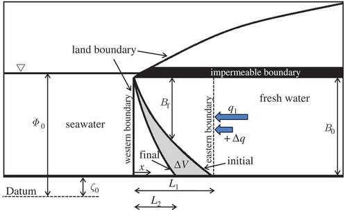
A useful point of reference for the scale of T_SWR is the characteristic time proposed by van Dam (1999) (hereafter referred to as T_ch), which can be interpreted as the time needed for the seawater volume, which is contained between the initial and the ultimate location of the interface (shaded area in Fig. 1), to be displaced into the sea:

(2) $T_{\mathrm{c}\mathrm{h}}=\frac{\mathrm{\Delta }V}{\mathrm{\Delta }q}$(2)

where Δq = q₂ − q₁, and ΔV is the volume [L²] of the displaced seawater, if the interface, after an increase of the inflow at the inland boundary from q₁ to q₂, moves from its initial location to its final one (Fig. 1). Note that Equation (2) assumes that the seawater volume ΔV is displaced into the sea at a rate equal to Δq (i.e. the total increase of the inflow at the inland boundary). The latter simplifying assumption results in underestimation of the actual timescale of the phenomenon, i.e. T_ch < T_SWR (see Section 2.3), which indicates that T_ch can be considered only as a measure (see also remarks by van Dam 1999), and not as the exact duration of the SWR.

The interfaces at both initial and final locations are parabolas, for which the lengths of the saline wedge at the aquifer bottom L₁ and L₂ are (Strack 1976, Bear 1979):

(3) $L_i=\frac{K{B_0}^2}{2\text{δ}{q}_i},\mathrm{f}\mathrm{o}\mathrm{r}i=1,2$(3)

where K is the hydraulic conductivity [L T⁻¹], and

(4) $\delta =\frac{{\rho }_{\mathrm{f}}}{{\rho }_{\mathrm{s}}-{\rho }_{\mathrm{f}}}$(4)

with ρ_s and ρ_f being the densities [M L⁻³] of the saline and fresh groundwater, respectively; for ρ_s = 1025 kg/m³ and ρ_f = 1000 kg/m³, one obtains δ = 40.

Based on the latter, the volume ΔV of the displaced seawater results in:

(5) $\mathrm{\Delta }V=\frac{n{B}_0\left(L_1-L_2\right)}{3}$(5)

Using Equations (3)–(5), the characteristic measure of the timescale [T] for the final steady state to be established is obtained as:

(6) $T_{\mathrm{c}\mathrm{h}}=\frac{n{B}_0\left(L_1-L_2\right)}{3\mathrm{\Delta }q}=\frac{nK{B_0}^3}{6\text{δ}{q}_1{q}_2}$(6)

As shown in Sections 2.3 and 3, the latter physically-sound measure can be used effectively to analyse the dimensionless evolution of the considered phenomenon.

2.2 Numerical model

For the purposes of this study, a numerical model has been developed and utilized. It is a sharp interface model, in which the freshwater and seawater flow equations are integrated over the vertical (see Essaid 1990). The considered aquifer is homogeneous, its thickness is constant, there are no sources or sinks, and the flow direction is perpendicular to the coast (one-dimensional flow). The coupled freshwater and seawater flow equations are solved simultaneously, and the movement of the interface is dictated by the freshwater and seawater flow dynamics. Under the above assumptions, the depth-averaged continuity equations for the two fluids, combined with Darcy’s law, give (Bear 1979, Essaid 1990):

(7) $\left(S_{\mathrm{f}}{B}_{\mathrm{f}}+n\delta \right)\frac{\mathrm{\partial }{\mathrm{\Phi }}_{\mathrm{f}}}{\mathrm{\partial }t}-n\left(\delta +1\right)\frac{\mathrm{\partial }{\mathrm{\Phi }}_{\mathrm{s}}}{\mathrm{\partial }t}=K\frac{\mathrm{\partial }}{\mathrm{\partial }x}\left(B_{\mathrm{f}}\frac{\mathrm{\partial }{\mathrm{\Phi }}_{\mathrm{f}}}{\mathrm{\partial }x}\right)$(7)

(8) $\left(S_s{B}_{\mathrm{s}}+n(\delta +1)\right)\frac{\mathrm{\partial }{\mathrm{\Phi }}_{\mathrm{s}}}{\mathrm{\partial }t}-n\delta \frac{\mathrm{\partial }{\mathrm{\Phi }}_{\mathrm{f}}}{\mathrm{\partial }t}=K\frac{\mathrm{\partial }}{\mathrm{\partial }x}\left(B_{\mathrm{s}}\frac{\mathrm{\partial }{\mathrm{\Phi }}_{\mathrm{s}}}{\mathrm{\partial }x}\right)$(8)

in which f and s indices refer to the freshwater and the seawater, respectively; and where Φ_f(x,t) and Φ_s(x,t) are, respectively, the depth-averaged hydraulic freshwater and seawater heads [L]; B_f(x,t) and B_s(x,t) are, respectively, the freshwater and seawater thicknesses [L] (Fig. 1); and S_f and S_s are, respectively, the freshwater and seawater specific storage [L⁻¹]. Note that we assume that the hydraulic conductivity does not depend on the salinity; i.e. K_f = K_s = K. The system in Equations (7) and (8) constitutes a coupled system of two nonlinear, partial (second-order) differential equations, with four unknown dependent variables: Φ_f, Φ_s, B_f and B_s.

In addition, considering continuity of pressure at any point of the interface, one concludes:

(9) ${\zeta }_1=\left(1+\delta \right){\mathrm{\Phi }}_{\mathrm{s}}-\delta {\mathrm{\Phi }}_{\mathrm{f}}$(9)

where ζ₁(x,t) is the elevation of the interface, measured from an arbitrary level of reference, and is related to B_f and B_s, as follows (Fig. 1; for simplicity ζ₀ can be considered zero):

(10) $B_{\mathrm{f}}={\zeta }_0+B_0-{\zeta }_1$(10)

(11) $B_{\mathrm{s}}={\zeta }_1-{\zeta }_0$(11)

Using Equations (9)–(11), the unknown variables in (7) and (8) are theoretically reduced to two: Φ_f and Φ_s.

For the seaward boundary, constant hydraulic heads are imposed for both fluids (see also Cheng et al. 2000, Park and Aral 2004). At the landward boundary, a freshwater inflow, linearly increasing from q₁ to q₂ = q₁+ Δq is considered, whereas the seawater inflow is zero. The time interval for the inflow to increase from q₁ to q₂ is referred to as Δt_Δq.

Equations (7) and (8) combined with the boundary conditions can be written in the form:

(12) ${\mathit{C}}_{2m\times 2m}{\mathit{U}}_{2m\times 1}={\mathit{B}}_{2m\times 1}$(12)

where C is the coefficient matrix, U is a vector containing the unknown freshwater and seawater heads, B is a vector with known right-hand-side values, and m is the number of grid points in the x-direction.

The system in Equation (12) is solved at each time level utilizing a finite-differences scheme (Crank and Nicolson 1947), and, apart from the hydraulic heads in U, the location of the interface is also determined using Equation (9); thus the movement of the saline wedge through time is obtained. For more details on the numerical scheme, the reader is referred to the study by Essaid (1990).

2.3 Model consistency – SWR example

The accuracy with which the numerical scheme simulates the movement of the interface is of high importance for developing solid estimates for the SWR timescales. Because the adopted numerical scheme has not been tested in SWR processes (Essaid 1990), in this section we test its consistency under the conditions of the SWR process described in Section 2.1, by performing simulations with different spatio-temporal model discretization, focusing on (a) the sensitivity of the estimated values of T_SWR to the model resolution and (b) the overall model error, which is based on specific integrated criteria (see also analyses by Refsgaard 1997, Henriksen et al. 2003). The latter is done for a base SWR case in a confined, homogeneous and isotropic aquifer (Fig. 1), the characteristics of which are provided in Table 1.

Table 1. Physical parameter values of the base case.

Parameter	n (−)	Sf (m^−1)	K (m/d)	B0 (m)	q1 (m^2/d)	q2 (m^2/d)	L1 (m)	L2 (m)
Value	0.1	0.0030	0.2	10	0.02	0.16	12.5	1.56

Figure 2 shows the retreating interface, using Δx = 0.1 m and Δt = 0.3 d. To create the initial steady-state conditions, we use a period of 5 days, in which we run the model with a constant flux q₁ at the landside boundary. At time t = 5 d, a linear-in-time increase of the freshwater inflow is applied at the inland boundary of the aquifer, while for t ≥ 10 d, the inflow remains constant and equal to q₂ (so Δt_Δq = 5 d). The variation of the inflow from q₁ to q₂ makes the saline wedge retreat, and the toe of the interface moves from L₁ = 12.5 m to the asymptotic location L₂ = 1.56 m (Equation (3)).

Figure 2. Location of the freshwater–seawater interface through time: solid black lines correspond to the initial and final steady states, while grey lines correspond to t = 13, 26, 39, … d. The dashed line indicates the section at x = 0.5 m, where the outflow to the sea is numerically calculated (see Section 2.3); Δx = 0.1 m and Δt = 0.3 d.

In Figure 3, the location of the toe of the saline wedge is shown as a function of time for two different spatial resolutions. For t < 5 d, the toe is constant, because the freshwater inflow is still equal to q₁, thus the initial steady state is valid. For t > 5 d, the toe starts to retreat, approaching the point of the final steady state. However, due to the asymptotic nature of the final steady state, and the finite number of grid points in the x-direction, the theoretically final location is not occupied, which justifies the use of Equation (1) to estimate T_SWR. Moreover, as shown in Figure 3, the toe of the seawater wedge exhibits a stepwise movement through time, with steps becoming more distinct as the value of Δx increases. However, this does not affect the estimation of T_SWR considerably: in both cases a value of about 90  d is apparent (this is also consistent with Fig. 2). Also note that the timescale of the process results to be 3–4 times higher than the characteristic time in Equation (6) (Fig. 3), which justifies that the latter can be used to determine a rough measure of SWR timescales, but not the exact duration. Similar findings are shown in Table 2, where the values of T_SWR are provided for Δx = 0.1 and 0.5 m, with Δt varying from 0.1 to 2 d. All estimates are of the order of 90 d, which indicates that estimated T_SWR are quite robust.

Table 2. Consistency measures and T_SWR for different values of Δx and Δt. WB: water balance; DSV: displaced seawater volume.

Δx (m)	0.5			0.1
Δt (d)	2	1	0.5	0.5	0.3	0.1
WB (%)	28.3	27.4	26.9	1.3	1.4	1.5
DSV (%)	3.5	0.4	0.1	2.8	2.7	2.6
TSWR (d)	88.0	87.0	86.7	88.0	86.7	85.4

Figure 3. Location of the toe of the interface through time (black and grey lines). Dashed lines correspond to the time when the flux variation starts (T_start = 5 d), the characteristic time of the phenomenon in Equation (6), and the theoretical location of the toe in the final steady state (L₂ = 1.56 m).

For the overall evaluation of the model, we used the following water balance measures:

The error in the total water balance WB (%), defined as:

(13) $WB\left(\mathrm{\%}\right)=\frac{\left|V^{\mathrm{i}\mathrm{n}}-V^{\mathrm{o}\mathrm{u}\mathrm{t}}\right|}{V^{\mathrm{i}\mathrm{n}}}=\frac{\left|V_{\mathrm{f}}^{\mathrm{i}\mathrm{n}}-V_{\mathrm{f}}^{\mathrm{o}\mathrm{u}\mathrm{t}}-V_{\mathrm{s}}^{\mathrm{o}\mathrm{u}\mathrm{t}}\right|}{V_{\mathrm{f}}^{\mathrm{i}\mathrm{n}}}=\frac{\left|{\int }_0^{T_{\mathrm{S}\mathrm{W}\mathrm{R}}}{q}_{\mathrm{f},\mathrm{i}\mathrm{n}}dt-{\int }_0^{T_{\mathrm{S}\mathrm{W}\mathrm{R}}}{q}_{\mathrm{f},\mathrm{o}\mathrm{u}\mathrm{t}}dt-{\int }_0^{T_{\mathrm{S}\mathrm{W}\mathrm{R}}}{q}_{\mathrm{s},\mathrm{o}\mathrm{u}\mathrm{t}}dt\right|}{{\int }_0^{T_{\mathrm{S}\mathrm{W}\mathrm{R}}}{q}_{\mathrm{f},\mathrm{i}\mathrm{n}}dt}$(13)

where the superscripts in and out indicate, respectively, inflow to and outflow from the aquifer, while s and f refer, respectively, to the freshwater and seawater volume (V) or flux (q). Note that in Equation (13) the term for the change of water storage is neglected, due to the small value of the specific storage (see Table 1).

The error DSV (%) in the seawater volume displaced from the aquifer into the sea that is simulated by the numerical scheme, compared to its theoretical value given in Equation (5) is:

(14) $DSV\left(\mathrm{\%}\right)=\frac{\left|V_s^{\mathrm{o}\mathrm{u}\mathrm{t}}-0.95\mathrm{\Delta }V\right|}{0.95\mathrm{\Delta }V}=\frac{\left|{\int }_0^{T_{\mathrm{S}\mathrm{W}\mathrm{R}}}{q}_{\mathrm{s},\mathrm{o}\mathrm{u}\mathrm{t}}\mathrm{d}t-0.95\mathrm{\Delta }V\right|}{0.95\mathrm{\Delta }V}$(14)

where the coefficient 0.95 is used due to the fact that, in contrast to Equation (5), the process is considered to be terminated before the retreating interface reaches the final steady-state position (see Equation (1)). The consideration of the measure DSV (in addition to WB) ensures that small values of WB are not due to cancelling out possible errors in the numerically estimated fluxes q_f,out and q_s,out.

The temporal variation of the fluxes q_f,in, q_f,out and q_s,out for the selected case (see Table 1) are given in Figure 4, using Δx = 0.1 m and Δt = 0.3 d. The evolution of the term q_f,in is defined a priori and known (black line in Fig. 4), while q_f,out and q_s,out (grey solid and dashed lines, respectively) are calculated at each time step by means of Darcy’s law, using a central-difference derivative to estimate the $\frac{\mathrm{\partial }{\mathrm{\Phi }}_{\mathrm{f}}}{\mathrm{\partial }x}$ and $\frac{\mathrm{\partial }{\mathrm{\Phi }}_{\mathrm{s}}}{\mathrm{\partial }x}$ gradients, respectively. Since the Ghyben-Herzberg assumption results in zero aquifer thickness and infinite freshwater hydraulic gradient at the sea boundary, evaluation of q_f,out at x = 0 m is theoretically non-feasible; thus, we calculate $\frac{\mathrm{\partial }{\mathrm{\Phi }}_{\mathrm{f}}}{\mathrm{\partial }x}$ and $\frac{\mathrm{\partial }{\mathrm{\Phi }}_{\hat{\mathrm{s}}}}{\mathrm{\partial }x}$ at a section 0.5 m landward from the western boundary (Fig. 2). Due to the latter, DSV values include an additional small error, because a small fraction (i.e. area enclosed by black lines and the section of x = 0.5 m in Fig. 2) of the seawater volume displaced into the sea is not considered. One can observe the linear increase of the freshwater inflow that is applied at the inland boundary from t = 5 d to t = 10 d, which consequently makes the groundwater outflow (fresh and saline water) at the western boundary increase. When the inland freshwater flux stops increasing, the maximum saline outflow is obtained, which is in accordance with the remarks by van Dam (1999). For t ~ 100 d, the seawater becomes stationary (q_s,out = 0), and q_f,in = q_f,out, both of which indicate that the system approaches the new steady-state conditions.

Figure 4. Freshwater inflow (eastern boundary: black line), freshwater outflow (western boundary: grey solid line) and seawater outflow (western boundary: grey dashed line) of the system through time. Outflows are calculated at x = 0.5 m and Δt_Δq = T_end – T_start = 5 d; Δx = 0.1 m and Δt = 0.3 d.

In Table 2 the values of WB and DSV are provided for the aquifer case in Figure 1 (see also Table 1). As a general observation, Δt changes seem not to significantly affect the values of the measures; while in contrast, Δx changes considerably affect the accuracy of the model, especially the WB values. WB is quite high in the case of Δx = 0.5 m (i.e. about 27%), while it reduces to only 1.5% for the case of Δx = 0.1 m. The reason for that is that the estimation of the gradient $\frac{\mathrm{\partial }{\mathrm{\Phi }}_{\mathrm{f}}}{\mathrm{\partial }x}$ for the calculation of q_f,out is less accurate for coarse space resolutions. DSV is less sensitive to the Δx value, and in all cases appears to be sufficiently small. The consistency of DSV is based on the fact that Φ_s is not as abrupt at the sea boundary as Φ_f is, which makes the approximation of q_s,out adequately accurate even for low-resolution grids (e.g. Δx = 0.5 m). Finally, similarly to the WB behaviour, we find that, for increased Δx values, the black and grey solid lines deviate from the expected matching, which is now apparent for t ≥ 100 d.

Similar levels of consistency of the numerical solution in terms of its robustness in estimating T_SWR and honouring the water balance were obtained for all simulations presented in the following sections.

3 Dimensional analysis

Most studies that investigate the timescales of coastal processes refer to specific cases of geometric and hydraulic conditions (Cartwright et al. 2004, Goswami and Clement 2007, Kiro et al. 2008, Chang and Clement 2012, Lu and Werner 2013), although, in practical applications, arguments and conclusions of more general validity are needed (Werner et al. 2013).

To gain some general insight on SWR timescales, in this section we explore the dimensionless problem of SWR in idealized systems (we consider systems that are similar to the one presented in Section 2.1; see also Fig. 1). In doing so, we (a) establish a dimensional analysis for the differential Equations (7) and (8); (b) identify the dimensionless parameters that affect the SWR process; and (c) determine the effect of the identified parameters on the dimensionless timescale of the SWR. This procedure allows us to obtain estimates of T_SWR that are of general validity, not restricted to specific hydraulic and geometric characteristics of the system and/or specific rates of change of the boundary conditions.

3.1 Dimensionless form of the differential equations

To identify the dimensionless parameters influencing the SWR process, we use T_ch and other characteristic quantities describing SWR to write the differential Equations (7) and (8) in dimensionless form.

In particular, we consider the dimensionless variables:

(15a) $t^{\ast }\equiv \frac{t}{T_{\mathrm{c}\mathrm{h}}}$(15a)

(15b) $x^{\ast }\equiv \frac{x-L_2}{L_1-L_2}$(15b)

(15c) ${{\mathrm{\Phi }}_{\mathrm{f},\mathrm{s}}}^{\ast }\left(x,t\right)\equiv \frac{{\mathrm{\Phi }}_{\mathrm{f},\mathrm{s}}}{{\mathrm{\Phi }}_0}$(15c)

(15d) ${B_{\mathrm{f},\mathrm{s}}}^{\ast }\left(x,t\right)\equiv \frac{B_{\mathrm{f},\mathrm{s}}}{B_0}$(15d)

where the use of the length L₁ – L₂ in Equation (15b) is motivated by the concluding remarks of Lu and Werner (2013), who highlighted its importance in determining the SWR timescale. Also, note that L₁ – L₂ controls the volume ΔV of the displaced seawater into the sea and consequently the time T_ch (see Equations (5) and (6) and van Dam 1999). Φ₀ ≠ 0 is the sea level measured from an arbitrary reference level.

By inserting the above equations in Equation (7), one gets the dimensionless form of the freshwater continuity equation (see Appendix A for complete derivations):

(16) $\left(\frac{S_{\mathrm{f}}{B}_0}{n\delta }{B_{\mathrm{f}}}^{\ast }+1\right)\frac{\mathrm{\partial }{{\mathrm{\Phi }}_{\mathrm{f}}}^{\ast }}{\mathrm{\partial }{t}^{\ast }}-\left(\frac{1}{\delta }+1\right)\frac{\mathrm{\partial }{{\mathrm{\Phi }}_{\mathrm{s}}}^{\ast }}{\mathrm{\partial }{t}^{\ast }}=\frac{2\frac{q_2}{q_1}}{3{\left(\frac{q_2}{q_1}-1\right)}^2}\frac{\mathrm{\partial }}{\mathrm{\partial }{x}^{\ast }}\left({B_{\mathrm{f}}}^{\ast }\frac{\mathrm{\partial }{{\mathrm{\Phi }}_{\mathrm{f}}}^{\ast }}{\mathrm{\partial }{x}^{\ast }}\right)$(16)

Similar considerations are valid for Equation (8).

Interestingly, although Equations (7) and (8) reveal that the process of SWR is a function of various parameters (see also parameters in Table 1), the use of the dimensionless variables in Equation (15) reduces the number of the aforementioned parameters, as shown in Equation (16), to two, namely: the dimensionless specific storage ${S_{\mathrm{f}}}^{\ast }=\frac{S_{\mathrm{f}}{B}_0}{n\delta }$, and the ratio q₂/q₁ of the final and initial values of the flux at the landside boundary, the value of which is larger than one. A third parameter results from the boundary conditions: it is the dimensionless duration of the flux variation Δt_Δq* = Δt_Δq/T_ch, where Δt_Δq is the time required for the flux at the landside boundary to increase from q₁ to q₂ (see Sections 2.2 and 2.3, Fig. 4). The last parameter is the ratio $\xi =\frac{B_0}{L_1-L_2}$, which compares the two characteristic lengths in the vertical and horizontal directions.

According to this analysis, the functional relationship between the dimensionless timescale of SWR and the dimensionless parameters takes the form:

(17a) ${T_{\mathrm{S}\mathrm{W}\mathrm{R}}}^{\ast }\equiv \frac{T_{\mathrm{S}\mathrm{W}\mathrm{R}}}{T_{\mathrm{c}\mathrm{h}}}=f\left({S_{\mathrm{f}}}^{\ast },\frac{q_2}{q_1},\mathrm{\Delta }{t_{\mathrm{\Delta }q}}^{\ast },\xi \right)$(17a)

The investigation of the functional relationship f in Equation (17a) follows (Section 3.2), and is performed by considering different combinations of S_f*, q₂/q₁, Δt_Δq* and ξ, solving the corresponding dimensional problems (unless otherwise stated, the values of n, S_f, K and q₁ are equal to those of the base case in Table 1) using the numerical scheme in Section 2.2, and calculating the dimensionless location of the toe of the saline wedge, X_T*, as a function of the dimensionless time t*:

(17b) ${X_{\mathrm{T}}}^{\ast }\equiv \frac{X_{\mathrm{T}}-L_2}{L_1-L_2}=g\left({S_{\mathrm{f}}}^{\ast },\frac{q_2}{q_1},\mathrm{\Delta }{t_{\mathrm{\Delta }q}}^{\ast },\xi ,t^{\ast }\right)$(17b)

For each set of values of S_f*, q₂/q₁, Δt_Δq* and ξ, T_SWR* is determined by satisfying the dimensionless form of Equation (1):

(17c) $\begin{array}{rl}& {X_{\mathrm{T}}}^{\ast }\left({T_{\mathrm{S}\mathrm{W}\mathrm{R}}}^{\ast }\right)\equiv g\left({S_{\mathrm{f}}}^{\ast },\frac{q_2}{q_1},\mathrm{\Delta }{t_{\mathrm{\Delta }q}}^{\ast },\xi ,{T_{\mathrm{S}\mathrm{W}\mathrm{R}}}^{\ast }\right)\\ & =0.05\end{array}$(17c)

3.2 Sensitivity analysis

3.2.1 The effect of S_f*

The specific storage S_f is given by (Bear 1979):

(18) $S_{\mathrm{f}}={\rho }_{\mathrm{w}}g\left(b_{\mathrm{p}}+n{b}_{\mathrm{w}}\right)$(18)

where ρ_w [M L⁻³] is the density of water, g [L T⁻²] is the acceleration of gravity, and b_p and b_w [L T² M⁻¹] are the compressibilities of the porous material and water, respectively.

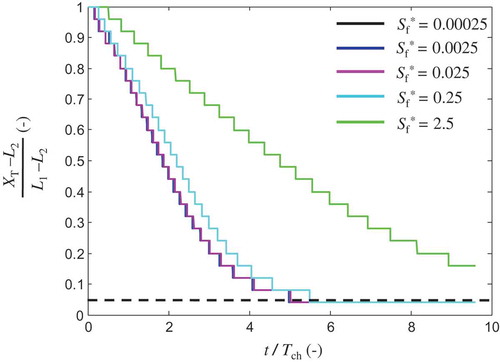
Very high values of S_f can be obtained for materials with high compressibility of the order of 10⁻⁷ m²/N (as is the case for clay; n = 0.4): the resulting specific storage S_f is of the order of 10⁻³ m⁻¹. Even for such aquifers, and for a thickness of up to B₀ = 200 m, S_f* is of the order of 0.01, which implies that the term S_f*B_f* is negligible compared to one, and therefore S_f* does not influence the SWR process, since the resulting term $\left({S_{\mathrm{f}}}^{\ast }{B_{\mathrm{f}}}^{\ast }+1\right)$ in Equation (16) is approximately constant and equal to unity. The latter result indicates that, in most applications, the term for the specific storage is of very low importance for the SWR and thus its effect can be neglected. In the unlikely case that the latter is not true, the timescale of the phenomenon would increase, since a larger freshwater volume is being stored in the aquifer and thus the saline wedge retreats more slowly. Evidently, as shown in Figure 5, where the simulated dimensionless location of the toe of the interface is given as a function of t* and S_f*, when S_f* is negligible relative to unity (black, blue and magenta lines), the results are almost identical, and for the selected values of q₂/q₁ and Δt_Δq*, a T_SWR* of the order of 4.5–5 is obtained. However, when S_f* = 0.25 (cyan line), that is comparable to unity, or even higher (green line), T_SWR* increases. Note though, that values of S_f* = 0.25 or higher are not likely in real applications, since they correspond to aquifers consisting of fine materials and with thickness much larger than 200 m.

Figure 5. Dimensionless distance of interface toe from its asymptotic location x = L₂ as a function of t* for different values of S_f*; q₂/q₁ = 2 and Δt_Δq* = 0.2. The dashed line illustrates the point that corresponds to 5% of the expected total shift of the toe: L₁ – L₂; see Equation (17c).

3.2.2 The effect of q₂/q₁

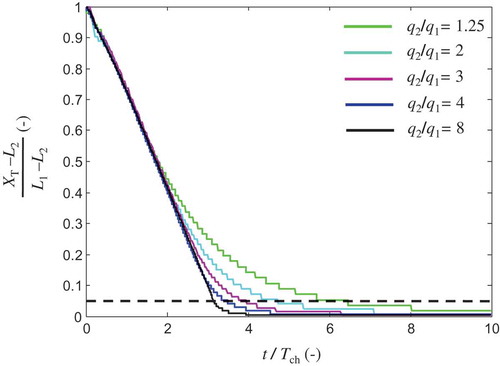
The dependence of the SWR on the value of the ratio q₂/q₁ is illustrated in Figure 6, where the dimensionless distance of the toe of the interface from the coast is presented as a function of t*, for different values of q₂/q₁. The results show that the smaller the increase of the inflow at the landside boundary, i.e. the smaller q₂/q₁ is, the larger T_SWR* is, while for t* < 2 the dimensionless image is almost the same, independent of the boundary conditions. More precisely, when q₂/q₁ = 8, one roughly obtains T_SWR* = 3.1, while for q₂/q₁ = 1.25, T_SWR* = 6.2. Similar conclusions can be obtained from Figure 7 (thick black line), where the dimensionless timescale of SWR is provided as a function of q₂/q₁. Note that when q₂/q₁ increases, T_SWR* decreases, while for low values of q₂/q₁, the curve is considerably more abrupt.

Figure 6. Dimensionless distance of interface toe from its asymptotic location x = L₂ as a function of t* for different values of ratio q₂/q₁; Δt_Δq* = 0.2.

3.2.3 The effect of Δt_Δq*

The effect of Δt_Δq* on the timescale T_SWR* is demonstrated in Figure 8. From the illustrations, it is obvious that as Δt_Δq* increases, SWR becomes slower (see also Fig. 3 in Lu and Werner 2013). Moreover, it is important to notice that when Δt_Δq* ≪ 1 (solid black and blue lines in Fig. 8) the results are identical, and correspond to the instantaneous case (Fig. 7). This result indicates that, in order for an inland flux change to be considered instantaneous (at least as far as the time response of SWR is concerned), Δt_Δq must be negligible relative to the characteristic time in Equation (6) (i.e. Δt_Δq* ≪ 1), which justifies the use of T_ch as a measure to analyse SWR (Equation (15a)). Otherwise, when Δt_Δq* ~ 1 (magenta line) or Δt_Δq* > 1 (cyan line), SWR becomes slower, while when Δt_Δq* ≫ 1 (green line), the timescale is of the same order as the flux variation time (i.e. T_SWR* ~ Δt_Δq*). This is theoretically consistent, since when the increase of the groundwater discharge toward the sea is very slow, it constitutes the slower mechanism driving the SWR; thus it dominates the timescale of the process (see also Lu and Werner 2013). In other words, because the inflow at the inland boundary increases very slowly, the system’s response is faster than the change of the boundary conditions through time. As a result, when the inland inflow stops increasing, the system reaches equilibrium; thus the T_SWR* is approximately equal to Δt_Δq*. One can observe this in Figure 9(a), where we provide the dimensionless form of Figure 4, for the case where Δt_Δq* = 10 (i.e. the green line in Fig. 8). Moreover, it is noticeable that these remarks are valid independent of the value of q₂/q₁, as indicated in Figure 9(b), where the same results as those of Figure 9(a) are presented, but for the case when q₂/q₁ = 2.

Figure 7. T_SWR* as a function of the ratio q₂/q₁ for instantaneous and non-instantaneous flux variations.

Figure 8. Dimensionless distance of interface toe from its asymptotic location x = L₂ as a function of t* for different values of Δt_Δq*; q₂/q₁ = 8.

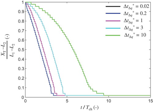
Figure 9. Dimensionless freshwater inflow (eastern boundary: black line), freshwater outflow (western boundary: grey solid line) and seawater outflow (western boundary: grey dashed line) as functions of t*; Δt_Δq* = 10 and (a) q₂/q₁ = 8, and (b) q₂/q₁ = 2.

Since in practical applications many flux variations may not be instantaneous (i.e. in many cases the condition Δt_Δq* ≪ 1 is not valid; see Dausman and Langevin 2005, Michael et al. 2005, Chang et al. 2011, Webb and Howard 2011), in Figure 7 we also include curves that refer to non-instantaneous changes of the freshwater inflow (thin lines), in an effort to illustrate the joint effect of both q₂/q₁ and Δt_Δq* on the SWR dynamics. In accordance with the remarks on Figure 8, one may observe that, as Δt_Δq* increases, the timescale of the process becomes larger. Also, the curves that refer to Δt_Δq* values larger than 10 tend to be approximately horizontal, which justifies the discussion of Figure 9.

3.2.4 The effect of ξ

Using Equation (3), one can easily show that:

(19) $\xi =\frac{B_0}{L_1-L_2}=\frac{1}{1-\frac{q_1}{q_2}}\frac{B_0}{L_1}=\frac{1}{1-\frac{q_1}{q_2}}\frac{2\delta q_1}{K{B}_0}=\frac{2\delta \theta }{1-\frac{q_1}{q_2}}$(19)

where θ$=\frac{q_1}{KB{}_0}$ is the hydraulic gradient at the landside boundary of the initial steady state. Note that B₀/L₁ and δθ correspond, respectively, to the aspect ratio and the discharge parameter in the Henry problem (Henry 1964). The latter compares viscous and buoyancy forces (Henry 1964, Dentz et al. 2006, Abarca et al. 2007). Equation (19) determines how the parameters ξ, B₀/L₁, θ and q₂/q₁ relate to each other and, since the effect of q₂/q₁ has already been taken into account in Figure 7, the extra effect of ξ (if any) is investigated by considering different values of the hydraulic gradient θ (e.g. 1% and 1‰), which also correspond to different aspect ratios B₀/L₁. We explore different values of θ by changing the value of K, and keeping all other dimensionless parameters constant. We present the results of the effect of θ for two cases: (a) q₂/q₁ = 1.25 and Δt_Δq* = 0.02, and (b) q₂/q₁ = 8 and Δt_Δq* = 15. The dimensionless evolution of the toe of the interface for different θ values is presented in Figure 10, revealing that its effect is negligible.

Figure 10. Dimensionless distance of interface toe from its asymptotic location x = L₂ as a function of t* for different values of θ.

4 Applicability in natural aquifers

In practical applications, the value of T_SWR* can be obtained from the type curves in Figure 7 for the values of q₂/q₁ and Δt_Δq* characterizing the system. Then, simply by using Equations (6) and (17a), the value of the actual timescale, T_SWR, can be calculated. However, since the results of Figure 7 have been obtained for idealized systems, the reliability of our estimates in real applications depends on the level to which the actual groundwater system can be approximated by the conceptual model in Section 2.1 (see Fig. 1) and the sharp interface assumption (i.e. cases where mixing between fresh groundwater and seawater is not important). Thus, before using the results of this study, these assumptions should be carefully taken into consideration. In this section, we try to gain insight into the effects of our main oversimplifying assumptions on the applicability of our estimates in real-world applications. We particularly discuss the effect of (a) the sharp interface assumption and (b) the homogeneity assumption. We also discuss the applicability of our results in unconfined aquifers.

4.1 Assessing the sharp interface assumption

In the case of important mixing, the definition of the toe placement, which is needed for the estimation of T_SWR, should be based on a definite isochlor (see Lu and Werner 2013), and consequently the relationship between the T_SWR values resulting from the two approximations (mixing and non-mixing fluids) is not ambiguous. To explore the applicability of our results in cases where mixing is relevant, we attempt a comparison with the results presented by Lu and Werner (2013), which also refer to confined aquifers and were obtained by assuming that (a) the longitudinal and transversal dispersivity values are a_L = 1 m and a_T = 0.1 m, respectively, and (b) the location of the toe of the seawater wedge is given by the 0.1 seawater concentration isochlor. In particular, we compare our estimates of T_SWR (based on Fig. 7) with those presented in Lu and Werner (2013, Figures 6, 9b and 10b) in Figures 11 and 12.

Figure 11. Comparison of our results (Fig. 7) with those of Lu and Werner (2013): (a) T_SWR as a function of the response length L₁ − L₂ for different initial conditions (water level differences: h_f-s = 0.75, 1, 1.25, 1.5, 1.75, 2 and 2.25 m) and inland head fluctuations (Δh_f = 0.1, 0.25, 0.5, 0.75, 1, 1.25, 1.5 and 2 m). Source: Lu and Werner (2013, Fig. 6). (b) T_SWR as a function of the response length L₁ − L₂ for different values of the ratio K/n = 16.67, 25, 33.33, 50 and 66.67 m/d. Source: Lu and Werner (2013, Fig. 9b).

Figure 12. Comparison of our results (Fig. 7) with those of Lu and Werner (2013): T_SWR as a function of the response length L₁ − L₂, for different values of longitudinal and transversal dispersivities: {a_L, a_T} = {1 m, 0.1 m}, {2 m, 0.2 m}, {5 m, 0.5 m}. Source: Lu and Werner (2013, Fig. 10b).

Figure 11(a) provides the timescales of the SWR in a head-controlled confined aquifer (solid lines, based on data in Lu and Werner 2013, Table 1–2), considering different initial conditions and inland head fluctuations. To take into account that our results (Figure 7) refer to flux variations (i.e. as opposed to head fluctuations) and the sharp interface assumption, for each case, the T_SWR estimate (circles in Fig. 11(a)) has been determined (see also Lu et al. 2015) as follows:

1. calculating the initial and final locations of the interface toe (in our study: L₁ and L₂, respectively) based on Equation (A.4) in Appendix A in Lu and Werner (2013), but using ${\epsilon }^{\prime }=\epsilon \left[1-{\left(\frac{a_{\mathrm{T}}}{B_0}\right)}^{\frac{1}{4}}\right]$ instead of $\epsilon =\frac{1}{\delta }$, to account for mixing effects on the level of penetration of the toe (see Pool and Carrera 2011, Lu and Werner 2013);

2. using the results from (i) to calculate q₁, q₂ (Equation (3)) and T_ch (Equation (6)); and

3. using the type curves in Figure 7 and Equations (6) and (17a), to calculate T_SWR, assuming instantaneous changes at the landside boundary.

Similar illustrations are given in Figure 11(b), which presents T_SWR for different values of the ratio K/n (cf. Lu and Werner 2013, Fig. 9b). Note that the value of the exponent in the dispersion correction (herein 1/4) depends on how the toe of the seawater wedge is defined (see assumption (b) above), as well as on whether an outflow gap is considered (Koussis et al. 2015).

The illustrated agreement presented in Figure 11 is an indication that mixing characterized by the assumptions (a) and (b) above leads to SWR timescales that do not differ significantly from those resulting from the approach of non-mixing fluids. This strengthens the validity of the results in Figure 7 also for cases where mixing takes place and dispersivity values are relatively small (see below).

Figure 12 illustrates the same comparison as Figure 11, but for different values of dispersivity (cf. Lu and Werner 2013, Fig. 10b). The explored cases correspond to longitudinal and transversal dispersivities: {a_L, a_T} = {1 m, 0.1 m}, {2 m, 0.2 m}, {5 m, 0.5 m}. This range of longitudinal dispersivities captures the range of values found in the majority of thin aquifers, and in thick aquifers with relatively high natural groundwater velocity (high hydraulic gradients at the landside boundary) and relatively low values of hydraulic conductivity (Kaleris and Ziogas 2013). In particular, Kaleris and Ziogas (2013) found that the longitudinal dispersivity in thin aquifers (B₀ ~ 10 m) varies from 0.95 m to 3.3 m, and in thick aquifers (B₀ ~ 100 m) from 4.7 to 16.5 m. Thus, the investigated range of dispersivity can be considered representative for a variety of practical applications.

The results show that as the dispersivity values increase, the validity of the results in Figure 7 becomes more approximate. This is expected, since, for higher values of dispersivity, the sharp interface assumption becomes less valid. In particular, the maximum difference of the two approaches based on the results in Figure 12 is of the order of 40%, and appears for the case when {a_L, a_T} = {5 m, 0.5 m}. This means that the estimates proposed herein could prove fruitful as first-order approximations of the SWR timescales for practitioners and decision makers in thin and thick aquifers. For longitudinal dispersivities higher than 5 m, our estimates are expected to be less reliable.

4.2 Assessing the homogeneity assumption

We attempt here to gain insight into the effect of heterogeneity on the timescale of the SWR, by analysing how the characteristic time proposed by van Dam (1999) (given in Equation (2)) changes in a heterogeneous system. For this purpose, we consider a coastal confined aquifer, where the hydraulic conductivity in the investigation area varies linearly in the flow direction. This is a simple form of gradual change of the hydraulic conductivity, which is a usual type of heterogeneity in natural aquifers (see Bear 1979), and is preferred here over the case of a vertically stratified heterogeneous aquifer, since our study refers to the depth-averaged problem of SWR (see Equations (7)–(8) and Appendix B).

Characterizing the hydraulic conductivity at the initial landside boundary (at x = L₁, see Fig. 1) as k_L1 and at x = 0 m as k₀, the hydraulic conductivity at any location 0 ≤ x ≤ L₁ is given by:

(20a) $K^{\mathrm{h}\mathrm{e}\mathrm{t}}\left(x\right)=\left(k_{\mathrm{L}1}-k_0\right)\frac{x}{L_1}+k_0$(20a)

or

(20b) $K^{\mathrm{h}\mathrm{e}\mathrm{t}}\left(x\right)=m_{\mathrm{k}}x+k_0$(20b)

where $m_{\mathrm{k}}=\frac{k_{\mathrm{L}1}-k_0}{L_1}$ is the change in hydraulic conductivity per unit length. Note that $m_{\mathrm{k}}$ can be negative, but because $K^{\mathrm{h}\mathrm{e}\mathrm{t}}\left(L_1\right)=m_{\mathrm{k}}{L}_1+k_0>0$, then

(20c) $m_{\mathrm{k}}>-\frac{k_0}{L_1}$(20c)

Based on the one-dimensional steady-state flow and the Ghyben-Herzberg approximation (Bear 1979), a heterogeneous aquifer as described above can be considered homogeneous for the problem of SWR when $\frac{m_{\mathrm{k}}{L}_1}{k_0}$ ~ 0 or $\frac{k_{\mathrm{L}1}-k_0}{k_0}$~ 0, and one can use the results in Figure 7 with K = k₀ (or K = k_L1) for estimating the duration of SWR (see Appendix B for analytical proof).

If the latter approximation is not valid, then the relationship between the characteristic time in Equation (2) of the heterogeneous aquifer and of a homogeneous model (with hydraulic conductivity K) is:

(21) $\frac{T{}_{\mathrm{c}\mathrm{h}}^{\mathrm{h}\mathrm{e}\mathrm{t}}}{T{}_{\mathrm{c}\mathrm{h}}^{\mathrm{h}\mathrm{o}\mathrm{m}}}=\frac{\frac{\mathrm{\Delta }{V}^{\mathrm{h}\mathrm{e}\mathrm{t}}}{\mathrm{\Delta }q}}{\frac{\mathrm{\Delta }{V}^{\mathrm{h}\mathrm{o}\mathrm{m}}}{\mathrm{\Delta }q}}=\frac{\mathrm{\Delta }{V}^{\mathrm{h}\mathrm{e}\mathrm{t}}}{\mathrm{\Delta }{V}^{\mathrm{h}\mathrm{o}\mathrm{m}}}$(21)

which gives (see Appendix B):

$\begin{array}{rl}& \frac{T_{\mathrm{c}\mathrm{h}}^{\mathrm{h}\mathrm{e}\mathrm{t}}}{T_{\mathrm{c}\mathrm{h}}^{\mathrm{h}\mathrm{o}\mathrm{m}}}=\\ & 3F^{\ast }\left(z\right)\left(1-H^{\ast }\left(z\right)\right)\frac{\left(z-1\right)-\left(z^{1/\lambda }-1\right)\frac{\left(1-H^{\ast }\left(z^{1/\lambda }\right)\right)}{\left(1-H^{\ast }\left(z\right)\right)}}{\left(1-1/\lambda \right)\left(z-1\right)}\frac{k_0}{K}\end{array}$

where:

$\begin{array}{rl}& F^{\ast }(z)=\frac{z-1}{lnz}\\ & H^{\ast }\left(z\right)={\int }_0^1\sqrt{\frac{1}{\mathrm{l}\mathrm{n}z}ln\left[\left(z-1\right)y+1\right]}dy\\ & z=\frac{k_{\mathrm{L}1}}{k_0}\mathrm{a}\mathrm{n}\mathrm{d}\lambda =\frac{q_2}{q_1}\end{array}$

or, more simply:

(22) $\frac{T_{\mathrm{c}\mathrm{h}}^{\mathrm{h}\mathrm{e}\mathrm{t}}}{T_{\mathrm{c}\mathrm{h}}^{\mathrm{h}\mathrm{o}\mathrm{m}}}=G\left(\frac{k_{\mathrm{L}1}}{k_0},\frac{q_2}{q_1}\right)\frac{k_0}{K}$(22)

Analytical derivation of the values of G is complicated (requires evaluation of the imaginary error function because of the integral H*) and goes beyond the scopes of this study. Instead, in Figure 13, we provide numerically calculated values of the ratio $\frac{T_{\mathrm{c}\mathrm{h}}^{\mathrm{h}\mathrm{e}\mathrm{t}}}{T_{\mathrm{c}\mathrm{h}}^{\mathrm{h}\mathrm{o}\mathrm{m}}}$, for $0<\frac{k_{L1}}{k_0}<10$, and $1<\frac{q_2}{q_1}<10$, and for three different homogeneous approximations. Note that for k_L1/k₀ = 1 (i.e. homogeneous case), the function G is not defined (see Equation (22), and notice the white vertical line in all three sub-plots of Fig. 13).

Figure 13. Values of the ratio T_ch^het/T_ch^hom given by Equation (22) for different q₂/q₁ and k_L1/k₀, when one approximates a heterogeneous aquifer with a homogeneous model: (a) K = k_L1, (b) K = k₀ and (c) K = (k₀ + k_L1)/2.

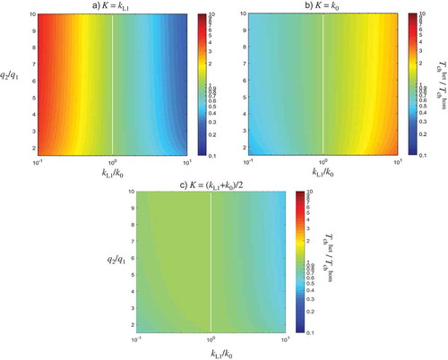
When using K = k_L1, the characteristic times $T{}_{\mathrm{c}\mathrm{h}}^{\mathrm{h}\mathrm{e}\mathrm{t}}$ and $T{}_{\mathrm{c}\mathrm{h}}^{\mathrm{h}\mathrm{o}\mathrm{m}}$ may differ significantly (by a factor larger than 3, i.e. $T_{\mathrm{c}\mathrm{h}}^{\mathrm{h}\mathrm{e}\mathrm{t}}/T_{\mathrm{c}\mathrm{h}}^{\mathrm{h}\mathrm{o}\mathrm{m}}>3$ for k_L1/k₀ <  0.3, or $T_{\mathrm{c}\mathrm{h}}^{\mathrm{h}\mathrm{e}\mathrm{t}}/T_{\mathrm{c}\mathrm{h}}^{\mathrm{h}\mathrm{o}\mathrm{m}}<0.3$ for k_L1/k₀ > 3; Fig. 13(a)). This is reasonable since k_L1 may be considered a representative value of hydraulic conductivity only for the initial steady state of the system, and not for the entire duration of the SWR phenomenon. Thus, the volume ΔV is significantly underestimated (overestimated) using this homogeneous approximation when k_L1/k₀ is really small (large), leading to underestimation (overestimation) of $T{}_{\mathrm{c}\mathrm{h}}^{\mathrm{h}\mathrm{e}\mathrm{t}}$ (Equation (21)). The choice of K = k₀ is better, and, in this case, lower discrepancies between the reality and the homogeneous approximation are apparent.

Interestingly, the results show that the characteristic time $T_{\mathrm{c}\mathrm{h}}^{\mathrm{h}\mathrm{e}\mathrm{t}}$ of a heterogeneous aquifer (as defined in Equation (2)) is of the same order of magnitude as the characteristic time $T{}_{\mathrm{c}\mathrm{h}}^{\mathrm{h}\mathrm{o}\mathrm{m}}$ calculated using a homogeneous model with K = (k₀ + k_L1)/2 and Equation (6). In particular, the ratio $\frac{T_{\mathrm{c}\mathrm{h}}^{\mathrm{h}\mathrm{e}\mathrm{t}}}{T_{\mathrm{c}\mathrm{h}}^{\mathrm{h}\mathrm{o}\mathrm{m}}}$ is very close to unity, and may vary from ~0.5 to ~1.2, depending on the q₂/q₁ and k_L1/k₀ values.

The changes in the characteristic time T_ch in heterogeneous aquifers that are discussed above provide some insight into the expected changes in the timescale of SWR under the influence of heterogeneity. However, the results of Figure 13 cannot be extrapolated to be used for the actual duration of SWR in heterogeneous aquifers, because the characteristic time T_ch in Equation (2) represents only a physically-sound measure and not the exact duration of the SWR.

4.3 Application in horizontal unconfined aquifers with no accretion

In the case of a horizontal unconfined aquifer, without accretion:

1. For δ ≫ 1 (as is usually the case), the length of seawater intrusion L_i can be approximated from Equation (3), and the corresponding characteristic time T_ch from Equation (6), with B₀ being the sea level measured from the bottom of the aquifer (see Bear 1979).

2. The system (7)–(8) takes the form (Essaid 1990):

$\left(S_{\mathrm{f}}{B}_{\mathrm{f}}+n\left(\delta +1\right)\right)\frac{\mathrm{\partial }{\mathrm{\Phi }}_{\mathrm{f}}}{\mathrm{\partial }t}-n\left(\delta +1\right)\frac{\mathrm{\partial }{\mathrm{\Phi }}_{\mathrm{s}}}{\mathrm{\partial }t}=K\frac{\mathrm{\partial }}{\mathrm{\partial }x}\left(B_{\mathrm{f}}\frac{\mathrm{\partial }{\mathrm{\Phi }}_{\mathrm{f}}}{\mathrm{\partial }x}\right)(7\ast )$

$\left(S_{\mathrm{s}}{B}_{\mathrm{s}}+n\left(\delta +1\right)\right)\frac{\mathrm{\partial }{\mathrm{\Phi }}_{\mathrm{s}}}{\mathrm{\partial }t}-n\delta \frac{\mathrm{\partial }{\mathrm{\Phi }}_{\mathrm{f}}}{\mathrm{\partial }t}=K\frac{\mathrm{\partial }}{\mathrm{\partial }x}\left(B_{\mathrm{s}}\frac{\mathrm{\partial }{\mathrm{\Phi }}_{\mathrm{s}}}{\mathrm{\partial }x}\right)(8\ast )$

and Equation (16) becomes:

$\left(\frac{S_{\mathrm{f}}{B}_0}{n\delta }{B}_{\mathrm{f}}^{\ast }+1+\frac{1}{\delta }\right)\frac{\mathrm{\partial }{{\mathrm{\Phi }}_{\mathrm{f}}}^{\ast }}{\mathrm{\partial }{t}^{\ast }}-\left(\frac{1}{\delta }+1\right)\frac{\mathrm{\partial }{{\mathrm{\Phi }}_{\mathrm{s}}}^{\ast }}{\mathrm{\partial }{t}^{\ast }}=\frac{2\frac{q_2}{q_1}}{3{\left(\frac{q_2}{q_1}-1\right)}^2}\frac{\mathrm{\partial }}{\mathrm{\partial }{x}^{\ast }}\left({B_{\mathrm{f}}}^{\ast }\frac{\mathrm{\partial }{{\mathrm{\Phi }}_{\mathrm{f}}}^{\ast }}{\mathrm{\partial }{x}^{\ast }}\right)(16\ast )$

Equations (8*) and (8) are identical, while in (7*), an extra term $n\frac{\mathrm{\partial }{\mathrm{\Phi }}_{\mathrm{f}}}{\mathrm{\partial }{t}^{\ast }}$ is added compared to (7) (similarly in (16*), $\frac{1}{\delta }\frac{\mathrm{\partial }{{\mathrm{\Phi }}_{\mathrm{f}}}^{\ast }}{\mathrm{\partial }{t}^{\ast }}$ is added). However, the latter is negligible compared to $n\delta \frac{\mathrm{\partial }{\mathrm{\Phi }}_{\mathrm{f}}}{\mathrm{\partial }t}$ for δ ≫ 1, and therefore Equations (7) and (7*), and (16) and (16*) can be considered identical.

Thus, because of (a) and (b) above, and provided that the depth of the aquifer differs slightly from B₀ (i.e. B_f(x,t) + B_s(x,t) ~ B₀, for all 0 ≤ t ≤ T_SWR and 0 ≤ x ≤ L₁), the timescale of SWR in horizontal unconfined aquifers without accretion can be sufficiently approximated by using the results of the confined aquifer presented in this study.

5 Conclusions

Investigation of SWR in coastal aquifers and of the associated timescales is an important and demanding subject in groundwater hydrology. Although of high importance to practitioners and decision makers, general and simple estimates of SWR timescales are not usually available. Indeed, because of the complexity of SWR, numerical tools are mainly utilized for analysing coastal dynamics, yet their results in most cases refer to specific hydraulic and geometric characteristics (see Cartwright et al. 2004, Lu and Werner 2013).

In this study, considering one-dimensional flow conditions in a confined and homogeneous coastal aquifer, and based on the sharp interface assumption, we performed a dimensional analysis for the governing equations of the SWR, which is triggered by the increase of the inflow at the landside aquifer boundary. The dimensionless parameters that affect the process have been identified, and their joint effect on the dimensionless duration of the SWR has been determined. To solve the coupled system of depth-averaged freshwater/seawater continuity equations, we utilized a numerical scheme proposed by Essaid (1990); while for defining the dimensionless timescale T_SWR* of SWR, we used a physically-based measure of the SWR timescale (T_ch in Equation (6)). The acceptability of the numerical solution was verified based on theoretical principles and appropriate criteria, while final results were also compared to previously reported results in the literature (van Dam 1999, Lu and Werner 2013).

Interestingly, the parameters affecting the dimensionless SWR-process resulted to be the following: (a) the ratio q₂/q₁ between the final and the initial values of the inflow at the landside aquifer boundary, for increased values of which, T_SWR* (i.e. the dimensionless timescale of SWR) decreases, and (b) the dimensionless duration of the flux variation Δt_Δq*, where in cases that Δt_Δq* ≪ 1, the SWR timescale is not affected, and the variation of the freshwater inflow can be considered instantaneous. When Δt_Δq* ~ 1, the movement of the interface becomes slower, while when Δt_Δq* ≫ 1, SWR is dominated by the boundary conditions, thus its dimensionless timescale is approximately equal to Δt_Δq*. The analysis also showed that, in common applications, the effect of the dimensionless specific storage S_f* and of the hydraulic gradient θ on the dimensionless SWR timescale is not significant.

Our investigation shows that solving the problem of SWR in the (T_ch, L₁–L₂) plane is very beneficial, since general estimates of the actual timescale of the SWR can be obtained based on simple type curves. In particular, using Figure 7, estimates can be obtained for any hydraulic and geometric characteristics in confined, homogeneous and isotropic aquifers with constant thickness, and for different rates of change of the boundary conditions. In our analysis, we also relaxed the sharp interface assumption, and it was indicated that the results of the present study can be consistent also in cases where the mixing between the freshwater and the seawater is considered, under the condition that dispersivity values are not very high. This concerns thin aquifers, as well as thick aquifers, in which the natural groundwater velocity toward the sea is relatively high and the hydraulic conductivity is relatively low. We also note that our analysis concerning heterogeneous aquifers gives insight into the effect of heterogeneity on the magnitude (not the actual duration) of SWR, and that our presented results can be used for sufficient approximations of SWR in homogeneous and isotropic horizontal unconfined aquifers with no accretion, provided that the depth of the aquifer varies slightly in space and time.

We conclude by saying that before applying our results to real-world applications, the assumptions of our analysis and our remarks in Section 4 need to be carefully considered. Yet, due to its simplicity, the presented approach can be used by practitioners as a tool for first-order approximating the SWR duration, before resorting to the use of numerical solvers, by approximating the properties of the real system with proper parameter values of the conceptual model considered here. In this way, our results may prove useful toward refining decision making and design policies for effective water management in coastal regions.

Acknowledgements

The authors would like to thank the associate editor Professor Aldo Fiori and two anonymous reviewers for their helpful comments and suggestions that greatly improved the manuscript.

Disclosure statement

No potential conflict of interest was reported by the authors.

Additional information

Funding

The work of Antonios Mamalakis was supported by LIFE (Linked Institutions for Future Earth) funded under NSF’s Science Across Virtual Institutes (SAVI) programme (NSF grant EAR-1242458).

Appendix A: Analytical derivation of Equation (16)

Consider again Equation (7):

(A1) $\left(S_{\mathrm{f}}{B}_{\mathrm{f}}+n\delta \right)\frac{\mathrm{\partial }{\mathrm{\Phi }}_{\mathrm{f}}}{\mathrm{\partial }t}-n\left(\delta +1\right)\frac{\mathrm{\partial }{\mathrm{\Phi }}_{\mathrm{s}}}{\mathrm{\partial }t}=K\frac{\mathrm{\partial }}{\mathrm{\partial }x}\left(B_{\mathrm{f}}\frac{\mathrm{\partial }{\mathrm{\Phi }}_{\mathrm{f}}}{\mathrm{\partial }x}\right)$(A1)

and Equation (15):

(A2a) $t^{\ast }\equiv \frac{t}{T_{\mathrm{c}\mathrm{h}}}$(A2a)

(A2b) $x^{\ast }\equiv \frac{x-L_2}{L_1-L_2}$(A2b)

(A2c) ${{\mathrm{\Phi }}_{\mathrm{f},\mathrm{s}}}^{\ast }\left(x,t\right)\equiv \frac{{\mathrm{\Phi }}_{\mathrm{f},\mathrm{s}}}{{\mathrm{\Phi }}_0}$(A2c)

(A2d) ${B_{\mathrm{f},\mathrm{s}}}^{\ast }\left(x,t\right)\equiv \frac{B_{\mathrm{f},\mathrm{s}}}{B_0}$(A2d)

By inserting Equations (A2) into Equation (A1), one gets:

$\left(S_{\mathrm{f}}{B_{\mathrm{f}}}^{\ast }{B}_0+n\delta \right)\frac{{\mathrm{\Phi }}_0}{T_{\mathrm{c}\mathrm{h}}}\frac{\mathrm{\partial }{{\mathrm{\Phi }}_{\mathrm{f}}}^{\ast }}{\mathrm{\partial }{t}^{\ast }}-n\left(\delta +1\right)\frac{{\mathrm{\Phi }}_0}{T_{\mathrm{c}\mathrm{h}}}\frac{\mathrm{\partial }{{\mathrm{\Phi }}_{\mathrm{s}}}^{\ast }}{\mathrm{\partial }{t}^{\ast }}=\frac{K{B}_0{\mathrm{\Phi }}_0}{{\left(L_1-L_2\right)}^2}\frac{\mathrm{\partial }}{\mathrm{\partial }{x}^{\ast }}\left({B_{\mathrm{f}}}^{\ast }\frac{\mathrm{\partial }{{\mathrm{\Phi }}_{\mathrm{f}}}^{\ast }}{\mathrm{\partial }{x}^{\ast }}\right)$

and dividing by Φ₀ ≠ 0:

$\left(S_{\mathrm{f}}{B}_0{B_{\mathrm{f}}}^{\ast }+n\delta \right)\frac{\mathrm{\partial }{{\mathrm{\Phi }}_{\mathrm{f}}}^{\ast }}{\mathrm{\partial }{t}^{\ast }}-n\left(\delta +1\right)\frac{\mathrm{\partial }{{\mathrm{\Phi }}_{\mathrm{s}}}^{\ast }}{\mathrm{\partial }{t}^{\ast }}=\frac{K{B}_0{T}_{\mathrm{c}\mathrm{h}}}{{\left(L_1-L_2\right)}^2}\frac{\mathrm{\partial }}{\mathrm{\partial }{x}^{\ast }}\left({B_{\mathrm{f}}}^{\ast }\frac{\mathrm{\partial }{{\mathrm{\Phi }}_{\mathrm{f}}}^{\ast }}{\mathrm{\partial }{x}^{\ast }}\right)$

Based on Equation (6):

$\left(S_{\mathrm{f}}{B}_0{B_{\mathrm{f}}}^{\ast }+n\delta \right)\frac{\mathrm{\partial }{{\mathrm{\Phi }}_{\mathrm{f}}}^{\ast }}{\mathrm{\partial }{t}^{\ast }}-n\left(\delta +1\right)\frac{\mathrm{\partial }{{\mathrm{\Phi }}_{\mathrm{s}}}^{\ast }}{\mathrm{\partial }{t}^{\ast }}=\frac{K{B_0}^2\frac{n}{3\left(q_2-q_1\right)}}{\left(L_1-L_2\right)}\frac{\mathrm{\partial }}{\mathrm{\partial }{x}^{\ast }}\left({B_{\mathrm{f}}}^{\ast }\frac{\mathrm{\partial }{{\mathrm{\Phi }}_{\mathrm{f}}}^{\ast }}{\mathrm{\partial }{x}^{\ast }}\right)$

Based on Equation (3):

$\left(S_{\mathrm{f}}{B}_0{B_{\mathrm{f}}}^{\ast }+n\delta \right)\frac{\mathrm{\partial }{{\mathrm{\Phi }}_{\mathrm{f}}}^{\ast }}{\mathrm{\partial }{t}^{\ast }}-n\left(\delta +1\right)\frac{\mathrm{\partial }{{\mathrm{\Phi }}_{\mathrm{s}}}^{\ast }}{\mathrm{\partial }{t}^{\ast }}=\frac{2\delta n}{3\left(\frac{1}{q_1}-\frac{1}{q_2}\right)\left(q_2-q_1\right)}\frac{\mathrm{\partial }}{\mathrm{\partial }{x}^{\ast }}\left({B_{\mathrm{f}}}^{\ast }\frac{\mathrm{\partial }{{\mathrm{\Phi }}_{\mathrm{f}}}^{\ast }}{\mathrm{\partial }{x}^{\ast }}\right)$

or

(A3) $\left(S_{\mathrm{f}}{B}_0{B_{\mathrm{f}}}^{\ast }+n\delta \right)\frac{\mathrm{\partial }{{\mathrm{\Phi }}_{\mathrm{f}}}^{\ast }}{\mathrm{\partial }{t}^{\ast }}-n\left(\delta +1\right)\frac{\mathrm{\partial }{{\mathrm{\Phi }}_{\mathrm{s}}}^{\ast }}{\mathrm{\partial }{t}^{\ast }}=\frac{2\delta n\frac{q_2}{q_1}}{3{\left(\frac{q_2}{q_1}-1\right)}^2}\frac{\mathrm{\partial }}{\mathrm{\partial }{x}^{\ast }}\left({B_{\mathrm{f}}}^{\ast }\frac{\mathrm{\partial }{{\mathrm{\Phi }}_{\mathrm{f}}}^{\ast }}{\mathrm{\partial }{x}^{\ast }}\right)$(A3)

Dividing Equation (A3) by δn, one gets Equation (16).

Appendix B: Complete derivations for assessing the homogeneity assumption (see Section 4.2)

We consider a coastal confined aquifer, where the hydraulic conductivity in the investigation area varies linearly. This is a simple form of gradual change of the hydraulic conductivity, which is a usual type of heterogeneity in natural aquifers (see Bear 1979).

Characterizing the hydraulic conductivity at the initial landside boundary (at x = L₁, Fig. 1) as k_L1 and at x = 0 m as k₀, the hydraulic conductivity at any location 0 ≤ x ≤ L₁ is given by:

(B1a) $K^{\mathrm{h}\mathrm{e}\mathrm{t}}\left(x\right)=\left(k_{\mathrm{L}1}-k_0\right)\frac{x}{L_1}+k_0$(B1a)

or:

(B1b) $K^{\mathrm{h}\mathrm{e}\mathrm{t}}\left(x\right)=m_{\mathrm{k}}x+k_0$(B1b)

where $m_{\mathrm{k}}=\frac{k_{\mathrm{L}1}-k_0}{L_1}$ is the change of the hydraulic conductivity per unit length. Note that $m_{\mathrm{k}}$ can be negative, but because $K^{\mathrm{h}\mathrm{e}\mathrm{t}}\left(L_1\right)=m_{\mathrm{k}}{L}_1+k_0>0$, then:

(B1c) $m_{\mathrm{k}}>-\frac{k_0}{L_1}$(B1c)

Based on the one-dimensional steady-state flow and the Ghyben-Herzberg approximation (Bear 1979), the Darcy’s law at any location 0 ≤ x ≤ L₁ predicts:

$q_1=K^{\mathrm{h}\mathrm{e}\mathrm{t}}\left(x\right)B_{\mathrm{f}}\left(x\right)\frac{\mathrm{\partial }{\mathrm{\Phi }}_{\mathrm{f}}}{\mathrm{\partial }x}$

where B_f is the thickness occupied by freshwater. Because ${\mathrm{\Phi }}_{\mathrm{f}}=\frac{B_{\mathrm{f}}}{\delta }$, then:

$q_1=\frac{1}{\delta }{K}^{\mathrm{h}\mathrm{e}\mathrm{t}}\left(x\right)B_{\mathrm{f}}\left(x\right)\frac{\mathrm{\partial }{B}_{\mathrm{f}}}{\mathrm{\partial }x}$

or

$\frac{\delta q_1}{K^{\mathrm{h}\mathrm{e}\mathrm{t}}\left(x\right)}=B_{\mathrm{f}}\left(x\right)\frac{\mathrm{\partial }{B}_{\mathrm{f}}}{\mathrm{\partial }x}$

or

$\int \frac{\delta q_1}{m_{\mathrm{k}}x+k_0}dx=\int B_{\mathrm{f}}d{B}_{\mathrm{f}}$

or

$\frac{\delta q_1}{m_{\mathrm{k}}}\mathrm{l}\mathrm{n}\left[m_{\mathrm{k}}x+k_0\right]=\frac{B_{\mathrm{f}}{\left(x\right)}^2}{2}+\mathrm{c}\mathrm{o}\mathrm{n}\mathrm{s}\mathrm{t}\mathrm{a}\mathrm{n}\mathrm{t}$

Because for x = 0, B_f = 0, then:

(B2) $B_{\mathrm{f}}{\left(x\right)}^2=\frac{2\delta q_1}{m_{\mathrm{k}}}ln\left[\frac{m_{\mathrm{k}}x}{k_0}+1\right]$(B2)

where $\frac{m_{\mathrm{k}}x}{k_0}+1>0$, for any location 0 ≤ x ≤ L₁ because of (B1c).

Using the approximation ln[w + 1] ~ w, if w ~ 0, one gets:

$B_{\mathrm{f}}{\left(x\right)}^2=\frac{2\delta q_1}{k_0}x$

$\mathrm{i}\mathrm{f}\frac{m_{\mathrm{k}}{L}_1}{k_0}\sim 0\mathrm{o}\mathrm{r}\frac{k_{\mathrm{L}1}-k_0}{k_0}\sim 0$

which corresponds to the homogeneous case, with conductivity value equal to k₀. Thus, L_i and T_ch of the heterogeneous aquifer can be approximated by Equations (3) and (6), respectively.

Moreover, equation (7) in a heterogeneous aquifer takes the form (see Essaid 1990; similar remarks are valid for Equation (8)):

$\left(S_{\mathrm{f}}{B}_{\mathrm{f}}+n\delta \right)\frac{\mathrm{\partial }{\mathrm{\Phi }}_{\mathrm{f}}}{\mathrm{\partial }t}-n\left(\delta +1\right)\frac{\mathrm{\partial }{\mathrm{\Phi }}_{\mathrm{s}}}{\mathrm{\partial }t}=\frac{\mathrm{\partial }}{\mathrm{\partial }x}\left(B_{\mathrm{f}}{K}^{\mathrm{h}\mathrm{e}\mathrm{t}}\frac{\mathrm{\partial }{\mathrm{\Phi }}_{\mathrm{f}}}{\mathrm{\partial }x}\right)$

or

$\left(S_{\mathrm{f}}{B}_{\mathrm{f}}+n\delta \right)\frac{\mathrm{\partial }{\mathrm{\Phi }}_{\mathrm{f}}}{\mathrm{\partial }t}-n\left(\delta +1\right)\frac{\mathrm{\partial }{\mathrm{\Phi }}_{\mathrm{s}}}{\mathrm{\partial }t}=K^{\mathrm{h}\mathrm{e}\mathrm{t}}\frac{\mathrm{\partial }}{\mathrm{\partial }x}\left(B_{\mathrm{f}}\frac{\mathrm{\partial }{\mathrm{\Phi }}_{\mathrm{f}}}{\mathrm{\partial }x}\right)+B_{\mathrm{f}}\frac{\mathrm{\partial }{K}^{\mathrm{h}\mathrm{e}\mathrm{t}}}{\mathrm{\partial }x}\frac{\mathrm{\partial }{\mathrm{\Phi }}_{\mathrm{f}}}{\mathrm{\partial }x}$

or

(B3) $\begin{array}{l}\left(S_{\text{f}}{B}_{\text{f}}+n\delta \right)\frac{\partial {\Phi }_{\text{f}}}{\partial t}-n\left(\delta +1\right)\frac{\partial {\Phi }_{\text{s}}}{\partial t}\\ =K^{\text{het}}\frac{\partial }{\partial x}\left(B_{\text{f}}\frac{\partial {\Phi }_{\text{f}}}{\partial x}\right)+B_{\text{f}}{m}_{\text{k}}\frac{\partial {\Phi }_{\text{f}}}{\partial x}\end{array}$(B3)

Considering the dimensionless problem, by inserting Equations (15) into Equation (B3), one gets:

$\begin{array}{rl}& \left(S_{\mathrm{f}}{B_{\mathrm{f}}}^{\ast }{B}_0+n\delta \right)\frac{{\mathrm{\Phi }}_0}{T_{\mathrm{c}\mathrm{h}}}\frac{\mathrm{\partial }{{\mathrm{\Phi }}_{\mathrm{f}}}^{\ast }}{\mathrm{\partial }{t}^{\ast }}-n\left(\delta +1\right)\frac{{\mathrm{\Phi }}_0}{T_{\mathrm{c}\mathrm{h}}}\frac{\mathrm{\partial }{{\mathrm{\Phi }}_{\mathrm{s}}}^{\ast }}{\mathrm{\partial }{t}^{\ast }}\\ & =\frac{K^{\mathrm{h}\mathrm{e}\mathrm{t}}{B}_0{\mathrm{\Phi }}_0}{{\left(L_1-L_2\right)}^2}\frac{\mathrm{\partial }}{\mathrm{\partial }{x}^{\ast }}\left({B_{\mathrm{f}}}^{\ast }\frac{\mathrm{\partial }{{\mathrm{\Phi }}_{\mathrm{f}}}^{\ast }}{\mathrm{\partial }{x}^{\ast }}\right)+\frac{B_0{m}_{\mathrm{k}}{\mathrm{\Phi }}_0}{L_1-L_2}{B_{\mathrm{f}}}^{\ast }\frac{\mathrm{\partial }{{\mathrm{\Phi }}_{\mathrm{f}}}^{\ast }}{\mathrm{\partial }{x}^{\ast }}\end{array}$

and dividing by Φ₀ ≠ 0:

$\begin{array}{rl}& \left(S_{\mathrm{f}}{B_{\mathrm{f}}}^{\ast }{B}_0+n\delta \right)\frac{\mathrm{\partial }{{\mathrm{\Phi }}_{\mathrm{f}}}^{\ast }}{\mathrm{\partial }{t}^{\ast }}-n\left(\delta +1\right)\frac{\mathrm{\partial }{{\mathrm{\Phi }}_{\mathrm{s}}}^{\ast }}{\mathrm{\partial }{t}^{\ast }}\\ & =\frac{K^{\mathrm{h}\mathrm{e}\mathrm{t}}{B}_0{T}_{\mathrm{c}\mathrm{h}}}{{\left(L_1-L_2\right)}^2}\frac{\mathrm{\partial }}{\mathrm{\partial }{x}^{\ast }}\left({B_{\mathrm{f}}}^{\ast }\frac{\mathrm{\partial }{{\mathrm{\Phi }}_{\mathrm{f}}}^{\ast }}{\mathrm{\partial }{x}^{\ast }}\right)+\frac{B_0{m}_{\mathrm{k}}{T}_{\mathrm{c}\mathrm{h}}}{L_1-L_2}{B_{\mathrm{f}}}^{\ast }\frac{\mathrm{\partial }{{\mathrm{\Phi }}_{\mathrm{f}}}^{\ast }}{\mathrm{\partial }{x}^{\ast }}\end{array}$

Based on Equation (6):

$\begin{array}{rl}& \left(S_{\mathrm{f}}{B}_0{B_{\mathrm{f}}}^{\ast }+n\delta \right)\frac{\mathrm{\partial }{{\mathrm{\Phi }}_{\mathrm{f}}}^{\ast }}{\mathrm{\partial }{t}^{\ast }}-n\left(\delta +1\right)\frac{\mathrm{\partial }{{\mathrm{\Phi }}_{\mathrm{s}}}^{\ast }}{\mathrm{\partial }{t}^{\ast }}\\ & =\frac{K^{\mathrm{h}\mathrm{e}\mathrm{t}}{B_0}^2\frac{n}{3\left(q_2-q_1\right)}}{\left(L_1-L_2\right)}\frac{\mathrm{\partial }}{\mathrm{\partial }{x}^{\ast }}\left({B_{\mathrm{f}}}^{\ast }\frac{\mathrm{\partial }{{\mathrm{\Phi }}_{\mathrm{f}}}^{\ast }}{\mathrm{\partial }{x}^{\ast }}\right)+\frac{n{m}_{\mathrm{k}}{B}_0^2}{3\left(q_2-q_1\right)}{B_{\mathrm{f}}}^{\ast }\frac{\mathrm{\partial }{{\mathrm{\Phi }}_{\mathrm{f}}}^{\ast }}{\mathrm{\partial }{x}^{\ast }}\end{array}$

Based on Equation (3):

$\begin{array}{rl}& \left(S_{\mathrm{f}}{B}_0{B_{\mathrm{f}}}^{\ast }+n\delta \right)\frac{\mathrm{\partial }{{\mathrm{\Phi }}_{\mathrm{f}}}^{\ast }}{\mathrm{\partial }{t}^{\ast }}-n\left(\delta +1\right)\frac{\mathrm{\partial }{{\mathrm{\Phi }}_{\mathrm{s}}}^{\ast }}{\mathrm{\partial }{t}^{\ast }}\\ & =\frac{K^{\mathrm{h}\mathrm{e}\mathrm{t}}2\delta n}{k_{0}3\left(\frac{1}{q_1}-\frac{1}{q_2}\right)\left(q_2-q_1\right)}\frac{\mathrm{\partial }}{\mathrm{\partial }{x}^{\ast }}\left({B_{\mathrm{f}}}^{\ast }\frac{\mathrm{\partial }{{\mathrm{\Phi }}_{\mathrm{f}}}^{\ast }}{\mathrm{\partial }{x}^{\ast }}\right)\\ & +\frac{2n\delta m_{\mathrm{k}}{L}_1}{3\left(\frac{q_2}{q_1}-1\right)k_0}{B_{\mathrm{f}}}^{\ast }\frac{\mathrm{\partial }{{\mathrm{\Phi }}_{\mathrm{f}}}^{\ast }}{\mathrm{\partial }{x}^{\ast }}\end{array}$

or

$\begin{array}{rl}& \left(S_{\mathrm{f}}{B}_0{B_{\mathrm{f}}}^{\ast }+n\delta \right)\frac{\mathrm{\partial }{{\mathrm{\Phi }}_{\mathrm{f}}}^{\ast }}{\mathrm{\partial }{t}^{\ast }}-n\left(\delta +1\right)\frac{\mathrm{\partial }{{\mathrm{\Phi }}_{\mathrm{s}}}^{\ast }}{\mathrm{\partial }{t}^{\ast }}\\ & =\left(\frac{m_{\mathrm{k}}x}{k_0}+1\right)\frac{2\delta n\frac{q_2}{q_1}}{3{\left(\frac{q_2}{q_1}-1\right)}^2}\frac{\mathrm{\partial }}{\mathrm{\partial }{x}^{\ast }}\left({B_{\mathrm{f}}}^{\ast }\frac{\mathrm{\partial }{{\mathrm{\Phi }}_{\mathrm{f}}}^{\ast }}{\mathrm{\partial }{x}^{\ast }}\right)\\ & +\frac{2n\delta m_{\mathrm{k}}{L}_1}{3\left(\frac{q_2}{q_1}-1\right)k_0}{B_{\mathrm{f}}}^{\ast }\frac{\mathrm{\partial }{{\mathrm{\Phi }}_{\mathrm{f}}}^{\ast }}{\mathrm{\partial }{x}^{\ast }}\end{array}$

Dividing by δn, and given that $\frac{m_{\mathrm{k}}{L}_1}{k_0}$ ~ 0 (and q₂/q₁ is not very close to 1; e.g. for q₂/q₁> 1.1), one gets exactly Equation (16). Thus, the dimensionless heterogeneous problem is identical to the homogeneous one. So a heterogeneous aquifer can be considered homogeneous for the problem of SWR when $\frac{m_{\mathrm{k}}{L}_1}{k_0}$~ 0 and one can use the results in Figure 7 with K = k₀ (or K = k_L1) for estimating the duration of SWR.

If the latter approximation is not valid, then (B2) results in (for x = L_i, B_f = B₀):

(B4) $L_i=\frac{B_0^2{k}_{\mathrm{L}\mathrm{i}}}{2\delta q_i}{F}_i=\frac{B_0^2{k}_0}{2\delta q_i}{F}_i^{\ast }$(B4)

with: $F_i=\frac{\frac{k_0}{k_{\mathrm{L}\mathrm{i}}}-1}{\mathrm{l}\mathrm{n}\frac{k_0}{k_{\mathrm{L}\mathrm{i}}}}$ and $F_i^{\ast }=\frac{\frac{k_{\mathrm{L}\mathrm{i}}}{k_0}-1}{\mathrm{l}\mathrm{n}\frac{k_{\mathrm{L}\mathrm{i}}}{k_0}}$, for i = 1, 2 (initial and final steady state)

From Equation (B4) one gets:

$\frac{L_1}{L_2}=\frac{F_1^{\ast }}{F_2^{\ast }}\frac{q_2}{q_1}$

Thus, Equation (B1a) becomes:

$k_{\mathrm{L}2}=\left(k_{\mathrm{L}1}-k_0\right)\frac{L_2}{L_1}+k_0=\left(k_{\mathrm{L}1}-k_0\right)\frac{F_2^{\ast }}{F_1^{\ast }}\frac{q_1}{q_2}+k_0\mathrm{o}\mathrm{r}$

$k_{\mathrm{L}2}=\left(k_{\mathrm{L}1}-k_0\right)\frac{\left(\frac{k_{\mathrm{L}2}}{k_0}-1\right)\mathrm{l}\mathrm{n}\frac{k_{\mathrm{L}1}}{k_0}}{\mathrm{l}\mathrm{n}\frac{k_{\mathrm{L}2}}{k_0}\left(\frac{k_{\mathrm{L}1}}{k_0}-1\right)}\frac{q_1}{q_2}+k_0\mathrm{o}\mathrm{r}$

$k_{\mathrm{L}2}=\left(k_{\mathrm{L}1}-k_0\right)\frac{\left(k_{\mathrm{L}2}-k_0\right)\mathrm{l}\mathrm{n}\frac{k_{\mathrm{L}1}}{k_0}}{\mathrm{l}\mathrm{n}\frac{k_{\mathrm{L}2}}{k_0}\left(k_{\mathrm{L}1}-k_0\right)}\frac{q_1}{q_2}+k_0\mathrm{o}\mathrm{r}$

$\frac{q_2}{q_1}=\frac{\mathrm{l}\mathrm{n}\left[\frac{k_{\mathrm{L}1}}{k_0}\right]}{\mathrm{l}\mathrm{n}\left[\frac{k_{\mathrm{L}2}}{k_0}\right]}\mathrm{o}\mathrm{r}$

$\mathrm{l}\mathrm{n}\left[\frac{k_{\mathrm{L}2}}{k_0}\right]=ln\left[{\left[\frac{k_{\mathrm{L}1}}{k_0}\right]}^{\frac{q_1}{q_2}}\right]\mathrm{o}\mathrm{r}$

(B5) $\frac{k_{\mathrm{L}2}}{k_0}={\left[\frac{k_{\mathrm{L}1}}{k_0}\right]}^{\frac{q_1}{q_2}}$(B5)

To calculate the ΔV we cannot use Equation (5), because the interfaces in the two steady states are not parabolas. For each steady state, from Equation (B2) the freshwater volume is (i = 1, 2):

$V_i=n{\int }_0^{L_i}{B}_{\mathrm{f}}\left(x\right)dx$

or

$V_i=n{\int }_0^{L_i}\sqrt{\frac{2\delta q_i}{m_{\mathrm{k}}}ln\left[\frac{m_{\mathrm{k}}x}{k_0}+1\right]}dx$

or

$V_i=n{\int }_0^{L_i}\sqrt{\frac{2\delta q_i{L}_i}{k_{\mathrm{L}\mathrm{i}}-k_0}ln\left[\frac{k_{\mathrm{L}\mathrm{i}}-k_0}{k_0}\frac{x}{L_i}+1\right]}dx$

or

$V_i=n{\int }_0^{L_i}\sqrt{\frac{B_0^2}{\frac{k_{\mathrm{L}\mathrm{i}}}{k_0}-1}{F}_i^{\ast }ln\left[\left(\frac{k_{\mathrm{L}\mathrm{i}}}{k_0}-1\right)\frac{x}{L_i}+1\right]}dx$

or

$V_i=n{\int }_0^{L_i}{L}_i\sqrt{\frac{B_0^2}{\frac{k_{\mathrm{L}\mathrm{i}}}{k_0}-1}{F}_i^{\ast }ln\left[\left(\frac{k_{\mathrm{L}\mathrm{i}}}{k_0}-1\right)\frac{x}{L_i}+1\right]}\frac{dx}{L_i}$

or

$V_i=n{B}_0{L}_i{\int }_0^1\sqrt{\frac{F_i^{\ast }}{\frac{k_{\mathrm{L}\mathrm{i}}}{k_0}-1}ln\left[\left(\frac{k_{\mathrm{L}\mathrm{i}}}{k_0}-1\right)y+1\right]}dy$

or

$V_i=n{B}_0{L}_i{\int }_0^1\sqrt{\frac{1}{\mathrm{l}\mathrm{n}\frac{k_{\mathrm{L}\mathrm{i}}}{k_0}}ln\left[\left(\frac{k_{\mathrm{L}\mathrm{i}}}{k_0}-1\right)y+1\right]}dy$

or

$V_i=n{B}_0{L}_i{H}_i^{\ast }$

with

$H_i^{\ast }={\int }_0^1\sqrt{\frac{1}{\mathrm{l}\mathrm{n}\frac{k_{\mathrm{L}\mathrm{i}}}{k_0}}ln\left[\left(\frac{k_{\mathrm{L}\mathrm{i}}}{k_0}-1\right)y+1\right]}dy$

and the seawater volume is:

$V_i^{\mathrm{s}\mathrm{e}\mathrm{a}}=n{B}_0{L}_i(1-H_i^{\ast })$

The relationship between the characteristic time in Equation (2) of the heterogeneous aquifer and of a homogeneous model (with hydraulic conductivity K) is:

$\frac{T_{\mathrm{c}\mathrm{h}}^{\mathrm{h}\mathrm{e}\mathrm{t}}}{T_{\mathrm{c}\mathrm{h}}^{\mathrm{h}\mathrm{o}\mathrm{m}}}=\frac{\frac{\mathrm{\Delta }{V}^{\mathrm{h}\mathrm{e}\mathrm{t}}}{\mathrm{\Delta }q}}{\frac{\mathrm{\Delta }{V}^{\mathrm{h}\mathrm{o}\mathrm{m}}}{\mathrm{\Delta }q}}=\frac{\mathrm{\Delta }{V}^{\mathrm{h}\mathrm{e}\mathrm{t}}}{\mathrm{\Delta }{V}^{\mathrm{h}\mathrm{o}\mathrm{m}}}$

or

$\frac{T_{\mathrm{c}\mathrm{h}}^{\mathrm{h}\mathrm{e}\mathrm{t}}}{T_{\mathrm{c}\mathrm{h}}^{\mathrm{h}\mathrm{o}\mathrm{m}}}=\frac{n{B}_0({L_1}^{\mathrm{h}\mathrm{e}\mathrm{t}}(1-H_1^{\ast })-{L_2}^{\mathrm{h}\mathrm{e}\mathrm{t}}(1-H_2^{\ast }))}{\frac{n{B}_0({L_1}^{\mathrm{h}\mathrm{o}\mathrm{m}}-{L_2}^{\mathrm{h}\mathrm{o}\mathrm{m}})}{3}}=3\frac{\frac{B_0^2{k}_0}{2\delta q_1}{F}_1^{\ast }(1-H_1^{\ast })-\frac{B_0^2{k}_0}{2\delta q_2}{F}_2^{\ast }(1-H_2^{\ast })}{\frac{B_0^{2}K}{2\delta q_1}-\frac{B_0^{2}K}{2\delta q_2}}$

or

$\frac{T_{\mathrm{c}\mathrm{h}}^{\mathrm{h}\mathrm{e}\mathrm{t}}}{T_{\mathrm{c}\mathrm{h}}^{\mathrm{h}\mathrm{o}\mathrm{m}}}=3F_1^{\ast }(1-H_1^{\ast })\frac{1-\frac{q_1}{q_2}\frac{\left({\left[\frac{k_{\mathrm{L}1}}{k_0}\right]}^{\frac{q_1}{q_2}}-1\right)\mathrm{l}\mathrm{n}\frac{k_{\mathrm{L}1}}{k_0}}{\frac{q_1}{q_2}\mathrm{l}\mathrm{n}\frac{k_{\mathrm{L}1}}{k_0}\left(\frac{k_{\mathrm{L}1}}{k_0}-1\right)}\frac{1-H_2^{\ast }}{1-H_1^{\ast }}}{1-\frac{q_1}{q_2}}\frac{k_0}{K}$

or

$\frac{T_{\mathrm{c}\mathrm{h}}^{\mathrm{h}\mathrm{e}\mathrm{t}}}{T_{\mathrm{c}\mathrm{h}}^{\mathrm{h}\mathrm{o}\mathrm{m}}}=3F^{\ast }\left(z\right)\left(1-H^{\ast }\left(z\right)\right)\frac{\left(z-1\right)-\left(z^{1/\lambda }-1\right)\frac{\left(1-H^{\ast }\left(z^{1/\lambda }\right)\right)}{\left(1-H^{\ast }\left(z\right)\right)}}{\left(1-1/\lambda \right)\left(z-1\right)}\frac{k_0}{K}$

where

$F^{\ast }\left(z\right)=\frac{z-1}{\mathrm{l}\mathrm{n}z}$

and

$H^{\ast }\left(z\right)=\underset{0}{\overset{1}{{\displaystyle \int }}}\sqrt{\frac{1}{\text{ln}z}\ln \left[\left(z-1\right)y+1\right]}dy$

and

$z=\frac{k_{\mathrm{L}1}}{k_0}\mathrm{a}\mathrm{n}\mathrm{d}\lambda =\frac{q_2}{q_1}$

which can be simplified to Equation (22).

References

- Abarca, E., et al., 2007. Anisotropic dispersive Henry problem. Advances in Water Resources, 30 (4), 913–926. doi:10.1016/j.advwatres.2006.08.005
- Bear, J., 1972. Dynamics of fluids in porous media. New York, NY: American Elsevier Publishing Company
- Bear, J., 1979. Hydraulics of Groundwater. New York: McGraw-Hill.
- Bear, J. and Dagan, G., 1964. Moving interface in coastal aquifers. Proceedings of the American Society of Civil Engineers, 99 (HY4), 193–215.
- Bocanegra, E., et al., 2010. State of knowledge of coastal aquifer management in South America. Hydrogeology Journal, 18, 261–267. doi:10.1007/s10040-009-0520-5
- Bokuniewicz, H., 2001. Toward a coastal ground-water typology. Journal of Sea Research, 46 (2), 99–108. doi:10.1016/S1385-1101(01)00074-0
- Brovelli, A., Mao, X., and Barry, D.A., 2007. Numerical modeling of tidal influence on density-dependent contaminant transport. Water Resources Research, 43, W10426. doi:10.1029/2006WR005173
- Burnett, W.C., Taniguchi, M., and Oberdorfer, J., 2001. Measurement and significance of the direct discharge of groundwater into the coastal zone. Journal of Sea ResEarch, 46 (2), 109–116. doi:10.1016/S1385-1101(01)00075-2
- Cartwright, N., Li, L., and Nielsen, P., 2004. Response of salt-freshwater interface in coastal aquifer to a wave-induced groundwater pulse: field observations and modelling. Advances in Water Resources, 27, 297–303. doi:10.1016/j.advwatres.2003.12.005
- Chang, S.W. and Clement, T.P., 2012. Experimental and numerical investigation of saltwater intrusions dynamics in flux-controlled groundwater systems. Water Resources Research, 48, W09527. doi:10.1029/2012WR012134
- Chang, S.W., et al., 2011. Does sea-level rise have an impact on saltwater intrusion? Advances in Water Resources, 34, 1283–1291. doi:10.1016/j.advwatres.2011.06.006
- Cheng, A.H.D., et al., 2000. Pumping optimization in saltwater-intruded coastal aquifers. Water Resources Research, 36 (8), 2155–2165. doi:10.1029/2000WR900149
- Crank, J. and Nicolson, P., 1947. A practical method for numerical evaluation of solutions of partial differential equations of the heat-conduction type. Proceedings of the Cambridge Philosophical Society, 43, 50–67.
- Dausman, A. and Langevin, C.D. 2005. Movement of the saltwater interface in the surficial aquifer system in response to hydrologic stresses and water-management practices. Broward County, FL: US Geological Survey Scientific Investigations Report 2004-5256, 73 pp.
- Dentoni, M., et al., 2015. A simulation/optimization study to assess seawater intrusion management strategies for Gaza Strip coastal aquifer (Palestine). Hydrogeology Journal, 23 (2), 249–264. doi:10.1007/s10040-014-1214-1
- Dentz, M., et al., 2006. Variable-density flow in porous media. Journal of Fluid Mechanics, 561, 209–235. doi:10.1017/S0022112006000668
- Diersch, H.-J.G. and Kolditz, O., 2002. Variable-density flow and transport in porous media: approaches and challenges. Advances in Water Resources, 25, 899–944. doi:10.1016/S0309-1708(02)00063-5
- Essaid, H.I., 1990. A multilayered sharp interface model of coupled freshwater and saltwater flow in coastal systems: model development and application. Water Resources Research, 26 (7), 1431–1454. doi:10.1029/WR026i007p01431
- Ferguson, G. and Gleeson, T., 2012. Vulnerability of coastal aquifers to groundwater use and climate change. Nature Climate Change, 2, 342–345. doi:10.1038/NCLIMATE1413
- Galeati, G., Gambolati, G., and Neuman, S.P., 1992. Coupled and partially coupled Eulerian-Lagrangian model of freshwater–seawater mixing. Water Resources Research, 28 (1), 149–165. doi:10.1029/91WR01927
- Ghyben, B.W., 1888. Nota in Verband met de Voorgenomen Putboring Nabij Amsterdam [Notes on the probable results ofthe proposed well drilling near Amsterdam]. The Hague: Tijdschrift vanhet Koninklijk Institunt van Ingeniers, 8–22.
- Goswami, R.R. and Clement, T.P., 2007. Laboratory-scale investigation of saltwater intrusion dynamics. Water Resources Research, 43, W04418. doi:10.1029/2006WR005151
- Henriksen, H.J., et al., 2003. Methodology for construction, calibration and validation of national hydrological model for Denmark. Journal of Hydrology, 280 (1–4), 52–71. doi:10.1016/S0022-1694(03)00186-0
- Henry, H.R., 1964. Effects of dispersion on salt encroachment in coastal aquifers. In: Cooper et al., eds. Sea water in coastal aquifers. Washington, DC: United States Government Printing Office, US Geological Survey Water-Supply Paper 1613-C, C70–C84.
- Herckenrath, D., Langevin, C.D., and Doherty, J., 2011. Predictive uncertainty analysis of a saltwater intrusion model using null-space Monte Carlo. Water Resources Research, 47, W05504. doi:10.1029/2010WR009342
- Herzberg, A., 1901. Die Wasserversorgung einiger Nordseebäder. Journal Gasbeleuchtung und Wasserversorgung, 44 (815–819), 842–844.
- Hunt, B., 1985. Some analytical solutions for seawater intrusion control with recharge wells. Journal of Hydrology, 80, 9–18. doi:10.1016/0022-1694(85)90072-1
- Kacimov, A.R. and Obnosov, Y.V., 2001. Analytical solution for a sharp interface problem in sea water intrusion into coastal aquifer. Proceedings of the Royal Society London. Series A: Mathematical, Physical and Engineering Sciences, 457, 3023–3038.
- Kacimov, A.R. and Sherif, M.M., 2006. Sharp interface, one-dimensional seawater intrusion into a confined aquifer with controlled pumping: analytical solution. Water Resources Research, 42, W06501. doi:10.1029/2005WR004551
- Kaleris, V., 2006. Submarine groundwater discharge: effects of hydrogeology and of near shore surface water bodies. Journal of Hydrology, 325, 96–117. doi:10.1016/j.jhydrol.2005.10.008
- Kaleris, V., 2007. The importance of submarine groundwater discharge for the pollution of the near shore sea water. In: eds., G. Di Silvio and S. Lanzoni. Electronic proceedings of the 32nd IAHR congress harmonizing the demand of art and nature in hydraulics. held 1–6 July 2007. Venice, Italy. Theme B1.c, Groundwater–Seawater interaction, paper B1.c-036 10.
- Kaleris, V., et al., 2002. Modelling submarine groundwater discharge: an example from the western Baltic Sea. Journal of Hydrology, 265 (1–4), 76–99. doi:10.1016/S0022-1694(02)00093-8
- Kaleris, V. and Ziogas, A.I., 2013. The effect of cutoff walls on saltwater intrusion and groundwater extraction in coastal aquifers. Journal of Hydrology, 476, 370–383. doi:10.1016/j.jhydrol.2012.11.007
- Kiro, Y., et al., 2008. Time response of the water table and saltwater transition zone to a base level drop. Water Resources Research, 44, W12442. doi:10.1029/2007WR006752
- Kourakos, G. and Mantoglou, A., 2009. Pumping optimization of coastal aquifers based on evolutionary algorithms and surrogate modular neural network models. Advances in Water Resources, 32, 507–521. doi:10.1016/j.advwatres.2009.01.001
- Koussis, A., et al., 2015. A correction for Dupuit-Forchheimer interface flow models of seawater intrusion in unconfined coastal aquifers. Journal of Hydrology, 525, 277–285. doi:10.1016/j.jhydrol.2015.03.047
- Kranenburg, C., 1986. A time scale for long-term salt water intrusion in well-mixed estuaries. Journal of Physical Oceanography, 16, 1329–1331. doi:10.1175/1520-0485(1986)016<1329:ATSFLT>2.0.CO;2
- Langevin, C.D., 2003. Simulation of submarine ground water discharge to a marine estuary: biscayne bay, Florida. Groundwater, 41 (6), 758–771. doi:10.1111/gwat.2003.41.issue-6
- Lecca, G. and Cau, P., 2009. Using a Monte Carlo approach to evaluate seawater intrusion in the Oristano coastal aquifer: a case study from the AQUAGRID collaborative computing platform. Physics and Chemistry of the Earth, 34, 654–661. doi:10.1016/j.pce.2009.03.002
- Lu, C., Chen, Y., and Luo, J., 2012. Boundary condition effects on maximum groundwater withdrawal in coastal aquifers. Groundwater, 50 (3), 386–393. doi:10.1111/gwat.2012.50.issue-3
- Lu, C. and Luo, J., 2010. Dynamics of freshwater–seawater mixing zone development in dual-domain formations. Water Resources Research, 46, W11601. doi:10.1029/2010WR009344
- Lu, C. and Werner, A.D., 2013. Timescales of seawater intrusion and retreat. Advances in Water Resources, 59, 39–51. doi:10.1016/j.advwatres.2013.05.005
- Lu, C., et al., 2015. A correction on coastal heads for groundwater flow models. Groundwater, 53, 164–170. doi:10.1111/gwat.2015.53.issue-1
- Luyun Jr., R., Momii, K., and Nakagawa, K., 2011. Effects of recharge wells and flow barriers on seawater intrusion. Groundwater, 49 (2), 239–249. doi:10.1111/gwat.2011.49.issue-2
- Mantoglou, A., 2003. Pumping management of coastal aquifers using analytical models of saltwater intrusion. Water Resources Research, 39 (12), 1335. doi:10.1029/2002WR0011891
- Michael, H.A., Mulligan, A.E., and Harvey, C.F., 2005. Seasonal oscillations in water exchange between aquifers and the coastal ocean. Nature, 436 (25). doi:10.1038/nature03935
- Naji, A., Cheng, A.H.-D., and Ouazar, D., 1998. Analytical stochastic solutions of saltwater/freshwater interface in coastal aquifers. Stochastic Hydrology and Hydraulics, 12, 413–430. doi:10.1007/s004770050028
- Park, C.H. and Aral, M.M., 2004. Multi-objective optimization of pumping rates and well placement in coastal aquifers. Journal of Hydrology, 290 (1–2), 80–99. doi:10.1016/j.jhydrol.2003.11.025
- Pool, M. and Carrera, J., 2011. A correction factor to account for mixing in Ghyben- Herzberg and critical pumping rate approximations of seawater intrusion in coastal aquifers. Water Resources Research, 47. doi:10.1029/2010WR010256
- Refsgaard, J.C., 1997. Parameterisation, calibration and validation of distributed hydrological models. Journal of Hydrology, 198 (1–4), 69–97. doi:10.1016/S0022-1694(96)03329-X
- Sivan, O., et al., 2005. Geochemical evolution and timescale of seawater intrusion into the coastal aquifer of Israel. Geochimica Cosmochimica Acta, 69 (3), 579–592. doi:10.1016/j.gca.2004.07.023
- Strack, O.D.L., 1976. A single-potential solution for regional interface problems in coastal aquifers. Water Resources Research, 12 (6), 1165–1174. doi:10.1029/WR012i006p01165
- Taniguchi, M., 2002. Tidal effects on submarine groundwater discharge into the ocean. Geophysical Research Letters, 29 (12). doi:10.1029/2002GL014987
- van Dam, J.C., 1999. Exploitation, restoration and management. In: Bear et al. ed., Seawater intrusion in coastal aquifers – concepts, methods and practices. Dordrecht: Kluwer Academic Publishers, 73–125.
- Vappicha, V.N. and Nagaraja, S.H., 1976. An approximate solution for the transient interface in a coastal aquifer. Journal of Hydrology, 31, 161–173. doi:10.1016/0022-1694(76)90027-5
- Watson, T.A., Werner, A.D., and Simmons, C.T., 2010. Transience of seawater intrusion in response to sea level rise. Water Resources Research, 46, W12533. doi:10.1029/2010WR009564
- Webb, M.D. and Howard, K.W.F., 2011. Modeling the transient response of saline intrusion to rising sea-levels. Groundwater, 49 (4), 560–569. doi:10.1111/j.1745-6584.2010.00758.x
- Werner, A.D., et al., 2013. Seawater intrusion processes, investigation, and management: recent advances and future challenges. Advances in Water Resources, 51, 3–26. doi:10.1016/j.advwatres.2012.03.004
- Werner, A.D. and Simmons, C.T., 2009. Impact of sea-level rise on sea water intrusion in coastal aquifers. Groundwater, 47 (2), 197–204. doi:10.1111/gwat.2009.47.issue-2
- Zhang, H., 1999. Analytical study of capture time to a horizontal well. Journal of Hydrology, 217, 46–54. doi:10.1016/S0022-1694(99)00013-X
- Zhang, Q., Volker, R.E., and Lockington, D.A., 2001. Influence of seaward boundary condition on contaminant transport in unconfined coastal aquifers. Journal of Contaminant Hydrology, 49, 201–215.