A fusion-based neural network methodology for monthly reservoir inflow prediction using MODIS products

ABSTRACT

A model fusion approach was developed based on five artificial neural networks (ANNs) and MODIS products. Static and dynamic ANNs – the multi-layer perceptron (MLP) with one and two hidden layers, general regression neural network (GRNN), radial basis function (RBF) and nonlinear autoregressive network with exogenous inputs (NARX) – were used to predict the monthly reservoir inflow in Mollasadra Dam, Fars Province, Iran. Leaf area index and snow cover from MODIS, and rainfall and runoff data were used to identify eight different combinations to train the models. Statistical error indices and the Borda count method were used to verify and rank the identified combinations. The best results for individual ANNs were combined with MODIS products in a fusion model. The results show that using MODIS products increased the accuracy of predictions, with the MLP with two hidden layers giving the best performance. Also, the fusion model was found to be superior to the best individual ANNs.

KEYWORDS:

• Model fusion
• MODIS
• artificial neural network
• monthly reservoir runoff
• leaf area index (LAI)
• snow cover
• Borda count method

Editor R. Woods Associate editor A. Viglione

1 Introduction

Short-, mid- and long-term prediction of monthly reservoir inflow helps to produce better policies for hydrologists and water managers and to reduce drought and flood losses (Rezaeianzadeh et al. 2016). Hence, hydrologists have attempted to find a solution to this issue. As a result of previous investigations, empirical, physical, conceptual and data-driven techniques have been developed and widely used for rainfall–runoff simulation (Jothiprakash and Magar 2012). The problem is that all of these models had high prediction errors. To reduce the various uncertainties and computational errors, some scholars have suggested combining, i.e. fusing the results of individual models (Lai et al. 2014). Moreover, large sets of rainfall and runoff data are required to simulate monthly and annual inflows. However, in some basins such data are not available. One solution to that problem is the use of other parameters as model inputs in addition to rainfall and runoff data. Remote sensing technology is a suitable and useful tool to provide other parameters as input to models. Hence, selecting an appropriate method and collecting the required data are of significant importance in hydrological modelling.

Artificial neural networks (ANNs), as the most popular type of data-driven technique, are commonly used in rainfall–runoff modelling (Mondal et al. 2012, Valipour et al. 2013, Cheng et al. 2015, Setiono and Hadiani 2015, Kumar et al. 2015, Piotrowski et al. 2016, Rezaeianzadeh et al. 2016, Shiau and Hsu 2016, Zeroual et al. 2016). Due to their flexibility in being able to manage and predict missing data, ANN models are preferred over other conventional methods (Sharma and Tiwari 2009, Siou et al. 2012, Zeroual et al. 2016). In the past two decades, ANN models have been widely employed to predict hydrological variables such as daily, weekly and monthly runoff (Rajurkar et al. 2004, Siou et al. 2012, Nigam et al. 2014, Nanda et al. 2016). Different types of ANN models, such as multi-layer perceptron (MLP) (Jain et al. 2004, Riadet al. 2004, Srinivasulu and Jain 2006, Rezaeian Zadeh et al. 2010, Dhamge et al. 2012, Rezaeianzadeh et al. 2013, Kumar et al. 2015), multi-layer back-propagation ANN (BPANN) (Agarwal and Singh 2004), back-propagation neural network (BPNN), radial basis function neural network (RBF) (Jayawardena and Fernando 1998, Lin and Chen 2004, Senthil Kumar et al. 2005, Lee et al. 2010, Dar 2017), feedforward back-propagation (FFBP) (Shiau and Hsu 2016), general regression neural network (GRNN) (Islam et al. 2001, Cigizoglu and Alp 2004, Aytek and Alp 2008, Gowda and Mayya 2014, Mishra et al. 2014, Tayyab et al. 2016, Modaresi et al. 2017) and rotated general regression neural network (RGRNN) (Irfan et al. 2016, Yin et al. 2016), have been applied for rainfall–runoff simulation. In recent years, dynamic ANN models have been suggested which are more efficient than static ANN models to obtain time series (Guzman et al. 2017). In dynamic ANN models, the computed outputs with a time delay are specified as the new input to the network (Valipour et al. 2013). A special type of recurrent, dynamic ANN model is the nonlinear autoregressive network with exogenous inputs (NARX). Recently, the NARX model has widely been used for hydrological applications, such as prediction of rainfall (Ang et al. 2014, Omidvar et al. 2015), floods (Ruslan et al. 2013, Nanda et al. 2016), water quality parameters (Chang et al. 2015), meteorological parameters (Lee and Tuan Resdi 2016) and groundwater levels (Chang et al. 2016, Guzman et al. 2017). Nevertheless, because of computational errors and various sources of uncertainty, application of these data-driven models for predicting hydrological parameters such as reservoir inflow often results in incorrect projections (Lai et al. 2014). Therefore, in recent years, some researchers have used a model fusion approach to reduce such errors (Abrahart and See 2002, Azmi et al. 2010, Ababaei et al. 2013, Khaleghi et al. 2013). As a follow-up to those studies, this study was aimed at developing a fusion neural network model based on five static and dynamic ANN models – MLP with one and two hidden layers, RBF, GRNN and NARX – to predict monthly reservoir inflows.

Different factors affect runoff, such as climatic variables (e.g. rainfall, temperature and potential evaporation) and human activities (e.g. land use). Among these parameters, rainfall is the most important factor (Huang et al. 2015). In most previous studies, rainfall data (Rajurkar et al. 2004), rainfall and runoff in the previous time steps (Jain et al. 2004, Srinivasulu and Jain 2006, Nourani et al. 2009, Kumar et al. 2015, Shiau and Hsu 2016), or meteorological parameters such as temperature and evapotranspiration (ET) (Okkan 2012, Bozorg-Haddad et al. 2016) have been used as inputs of ANN models. Rainfall and runoff data are usually sufficient to predict daily inflow rates, but longitudinal data are required for acceptable medium- and long-term (monthly and annual) runoff predictions, though these data may be unavailable for many basins. To solve this problem, other parameters may be addressed as inputs of ANN models. To this end, Sharma and Tiwari (2009) considered different characteristics of soil, topography, geomorphology, vegetation cover and monthly rainfall datasets. Engman (1997) mentioned that some parameters such as snow cover affect the hydrological regime. Roy et al. (2010) ignored snowmelt in their research on the main sources of error in runoff estimation models. The characteristics of vegetation cover, recorded by factors such as leaf area index (LAI), have an effective impact on runoff reduction as they may control the ET rate, especially in drought periods, but have rarely been considered in rainfall–runoff modelling (Daofeng et al. 2004, Yildiz and Barros 2007, Li et al. 2009). Considering vegetation cover data could improve runoff forecasts (Zhang et al. 2011). Compared to other vegetation indices, LAI has the highest correlation with hydrological variables and its application in runoff prediction models may help resolve uncertainties and improve results (Garcia-Quijano and Barros 2005, Fitch et al. 2010, Zhang et al. 2011, Zhou et al. 2013).

However, the data collection process is also an important issue once input data have been selected. Remote sensing is one of the more recent technologies used to obtain and extract the required information for water resources management (Gigante et al. 2009). There are many examples in the literature of using remote sensing data in hydrological modelling (Shrivastava et al. 2004, Milewski et al. 2009, Conesa-Garcia et al. 2010, Reshma et al. 2010, Sarmiento et al. 2012, Corona et al. 2014, Mahmoud 2014, Michailovsky and Bauer-Gottwein 2014, Samanta 2015). The moderate-resolution imaging spectroradiometer (MODIS) data have high resolution and more spectral bands. Georgievsky (2009) developed a model to predict river flow in Russia based on MODIS data and a snowmelt runoff model (SRM). Roy et al. (2010) used two hydrological models, the MOHYSE and Système de prévision hydrologique–apports verticaux (SPH-AV), together with MODIS and interactive multi-sensor snow and ice mapping system (IMS) snow cover products to estimate spring runoff. In another study, Zhou et al. (2013) used the MODIS-LAI in rainfall–runoff modelling. To investigate the relationships among vegetation indices and hydrological variables such as runoff coefficient, streamflow and ET, Fitch et al. (2010) used MODIS vegetation indices and conducted a comprehensive regression analysis. Zhang et al. (2008, 2010, 2011) used the MODIS-LAI to estimate ET in a simple lumped conceptual daily rainfall–runoff (SIMHYD) model. Li et al. (2009) and Zhou et al. (2013) applied hydrological models to estimate ET in the Xinanjiang model. Unlike the above-mentioned studies, which used remote sensing data in hydrological models, this study used remote sensing data as well as rainfall and runoff data as inputs to ANN models. Further, as previously stated, snow cover and vegetation cover are important input parameters in rainfall–runoff models, and remote sensing data are useful due to their spatial and temporal changes (Nagler et al. 2008). Therefore, snow cover and LAI data from the MODIS sensor were used as inputs of the ANN models in addition to rainfall and runoff data to predict monthly reservoir inflow.

In this study, five ANN models – the MLP with one and two hidden layers, GRNN and RBF neural networks as static ANN models and NARX as a dynamic ANN model – were selected and used to predict monthly reservoir inflow. Next, to obtain a more accurate inflow prediction, a fusion-based neural network approach using the best combination of individual ANN models was developed. The use of snow cover and LAI remote sensing data as input in runoff prediction models has been limited in previous studies of hydrological models (e.g. SRM, Xinanjiang, SIMHYD and SWAT) and, so far, such data have not been used as ANN model input. Furthermore, a fusion model based on ANN models using MODIS products as input data has not been reported before. The other goal of this study was to evaluate the effect of the application of MODIS LAI and snow cover data in addition to rainfall and runoff data from in situ stations as ANN model inputs to predict monthly reservoir inflow. The results of the ANN and fusion models were compared. This methodology is proposed for basins without long-term data series; to evaluate the proposed methodology, the study was conducted on Mollasadra Dam, Iran.

2 Methodology

This study was conducted to evaluate the accuracy of five static and dynamic ANN models (MLP with one and two hidden layers, GRNN, RBF and NARX) and a fusion-based neural network model to predict monthly reservoir inflow. Another goal of this study was to evaluate the effect of input parameters obtained from MODIS (LAI and snow cover) in addition to collected data on rainfall and runoff as required information to train the different types of ANN models. This structure is proposed to obtain a more accurate estimation of monthly reservoir inflow in basins without long-term data series. The flowchart of the proposed methodology is presented in Figure 1. In the first step, the Mollasadra basin in Fars Province, southwest Iran – a basin without long-term data series – was selected as a case study, and data were collected from raingauges and hydrometric stations. Runoff, rainfall, snow cover and LAI were specified as input data for a 15-year planning horizon of 2000–2015. In the second step, the autocorrelation function (ACF) and partial autocorrelation function (partial ACF) were used to determine the number of delays for each parameter and input combinations. In the next (third) step, the appropriate training and test datasets were determined using the Levene test and the T test. In Step 4, the training and testing of the five selected ANN models were carried out to predict the monthly reservoir inflow. In Step 5, the accuracy of each model was evaluated using the statistical error indices root mean square error (RMSE), mean absolute percentage error (MAPE), Willmott’s dimensionless index of agreement (d) and correlation coefficient (r). The combinations were then ranked by the Borda count method and the best input combination of each model was selected. Finally, in Step 6, for a more accurate prediction of monthly reservoir runoff, a fusion-based neural network model was developed. In this model, the outputs of the best combination of individual ANN models were utilized as input data of the MLP with one hidden layer, and the performance of the fusion-based model was compared with that of individual ANN models.

Figure 1. Algorithm of the proposed fusion-based neural network methodology for prediction of monthly reservoir inflow.

2.1 Case study

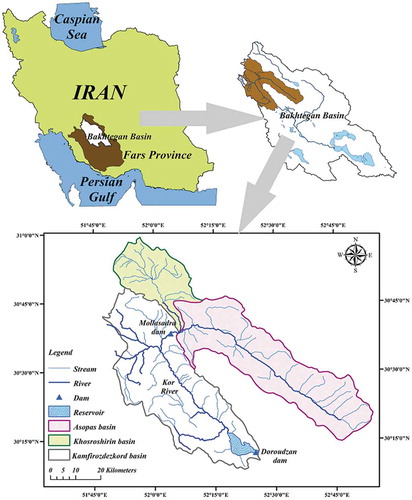
The Mollasadra watershed in Fars Province, Iran, is located on the Kor River, in the Bakhtegan basin between 51°50′–52°54′E and 30°14′–30°59′N. The location of the study area is shown in Figure 2. The Mollasadra Dam is a regulating earth-filled dam with length, height of crest and storage capacity of approx. 630 m, 72 m and 440 × 10⁶ m³ (MCM), respectively. This dam was designed to meet local needs for urban water supply and agricultural demand. The climate of the Bakhtegan basin is semi-arid and the average annual temperature, daily evaporation, precipitation, sunshine hours and frost days are equal to 5.5°C, 6.2 mm, 443 mm. 9.1 h and 54 d/year, respectively (Rezaeianzadeh et al. 2013, Nafarzadegan et al. 2018, Ghazali et al. 2018).

Figure 2. Location of study area (Mollasadra watershed) in the Bakhtegan basin, Iran.

2.2 Dataset

The rainfall and runoff amounts obtained from in situ stations and the LAI and snow cover data from the MODIS sensor were used as input data in the five selected ANN models. The monthly reservoir inflow rate of the hydrometric stations at the entrance of dam during the study period were collected from the Fars Regional Water Organization.

The results of Rezaeianzadeh et al. (2013) showed that, compared to spatially varied precipitation inputs, area-weighted precipitation data were superior. Using Thiessen polygons drawn around the raingauge stations for the two sub-basins (Asopas and Khosroshirin), the mean monthly precipitation for the Mollasadra watershed was estimated. The details and weights of the raingauge stations are shown in Table 1.

Table 1. Details of the raingauge stations used in this study.

Sub-basin	Station	Long. (°-′-ʺ)	Lat. (°-′-ʺ)	Thiessen weight
Asopas	Bidkal	52-37-31	30-09-57	0.002
	Dehkadeh-Sefid	52-04-59	30-42-55	0.098
	Dashtak	52-28-03	30-17-26	0.048
	Emamzadeh-Esmaeil	52-35-13	30-19-04	0.067
	Ahmad-Abad	52-41-26	30-23-21	0.413
	Sedeh	52-09-48	30-43-10	0.369
	Jamalbeyg	51-57-13	30-36-30	0.003
Khosroshirin	Dehkadeh-Sefid	52-04-59	30-42-55	0.242
	Sedeh	52-09-48	30-43-10	0.003
	Ghatar-Aghach	51-53-24	30-43-12	0.037
	Khosroshirin	52-00-39	30-54-05	0.587
	Dezkord	51-57-38	30-43-14	0.083
	Dehkadeh-Shahid	51-44-27	30-50-37	0.048

2.2.1 Snow cover area

The MODIS/Terra snow cover products MOD10A1 were used. The MODIS/Terra snow cover daily L3 global 500-m from 2000 to 2015 was provided by the National Snow and Ice Data Center (NSIDC; http://nsidc.org/data/mod10a1.html). The products were processed by ENVI® and MATLAB® software. In total, 5680 daily snow cover products were used and the mean monthly snow cover for 172 months (2000–2015) was calculated. The time series of snow cover changes in 2014 for the Mollasadra watershed is shown in Figure 3(a) as an example.

Figure 3. (a) Snow cover and (b) leaf area index (LAI) time series for the Mollasadra watershed in 2014.

2.2.2 Leaf area index (LAI)

Data used include MODIS/Terra 8-day LAI products (MOD15A2) at 1 km resolution for the period 2000–2015. These products are available from: https://ladsweb.nascom.nasa.gov.html. In total, 725 LAI products were used and the mean monthly LAI was calculated from four available products for each of 172 months (2000–2015). The products were also processed by ENVI® and MATLAB® software. As an example, the time series of LAI changes in 2014 for the Mollasadra watershed is shown in Figure 3(b).

2.3 Training and testing datasets

Based on Rezaeian Zadeh et al. (2010) and Rezaeianzadeh et al. (2016), the same distribution of mean-, high- and low-flow regimes was obtained using the Levene test and the T test for the training and testing stages. Different datasets were randomly generated and analysed for their variances by the Levene test. The p-value of the selected dataset was 0.528 (that is, >0.05 at the 95% confidence level). Based on the result of the Levene test it was assumed the variances are equal and the T test was carried out. The p-value of the T test was 0.557 (> 0.05) indicating that between training and testing datasets there is no statistically significant difference. A total of 121 monthly values (70% of the data) and 51 monthly values (30% of data) from the period 2000–2015 were used for training and testing the ANN models, respectively. The selected datasets for training and testing periods are shown in Figure 4.

2.4 Artificial neural networks (ANNs)

2.4.1 Multi-layer perceptron (MLP)

The most popular ANN model architecture nowadays is the MLP network (Rezaeian Zadeh et al. 2010, Albaradeyia et al. 2011). Simple neurons called perceptrons form the structure of this network. A single output is computed by a multi-layer perceptron according to the input weights and transfer functions from multiple inputs. The MLP neural network can be represented as follows:

(1) $y=v_0+{\sum }_{j=1}^J{v}_j.f\left({\sum }_{i=1}^n{w}_{ij}{x}_i+w_{j0}\right)$(1)

where y is a predicted value of the output, f is the activation function, J is the number of hidden units, n represents input variables, and w and v are MLP weights to be optimized.

In this study, two MLP neural networks were used: MLP1 with one hidden layer (one input layer, one hidden layer, one output layer) and MLP2 with two hidden layers (one input layer, two hidden layers, one output layer).

2.4.2 Radial basis function (RBF)

The RBF is an effective ANN model that was introduced by Powell (1987) for interpolating and simulating multidimensional fields (Sahin 1997, Tayyab et al. 2016). The type of connection between the hidden layer and inputs in the RBF network are not weighted and there are radially symmetric transfer functions on the hidden layer nodes (Jayawardena and Fernando 1998). There are several basic functions for training the RBF but, from the point of view of RBF performance, the type chosen is not crucial and the Gaussian function is the most common (Jayawardena and Fernando 1998, Balouchi et al. 2015, Tayyab et al. 2016). The output vector (y_j) from input vector (X) can be given by (Balouchi et al. 2015):

(2) $y_j=f\left\{\frac{∥X-U_j∥}{2{\sigma }_j^2}\right\}$(2)

where j is number of hidden nodes, U_j and $∥\ast ∥$ are the centre and Euclidian norm, respectively, of the jth RBF; and $({\sigma }_j^2)$ is the spread of the basis function.

The output of network Z_m at the mth output node in the RBF network is given by:

(3) $Z_m=f(X)={\sum }_{j=1}^{j=p}{y}_j{w}_{mj}$(3)

where w is the weight between output and hidden nodes.

2.4.3 General regression neural network (GRNN)

The GRNN introduced by Specht (1991) is a type of ANN model (Specht 1991). This model is defined based on the RBF model and has four layers: the input layer, the RBF (or pattern) layer, the summation layer and the output layer (Tayyab et al. 2016, Yin et al. 2016). The Gaussian function (Equation (2)) is implemented in the RBF layer. The amount of spread in this model is in the range of > 0, and should be determined by the user by the trial-and-error method; the typical amount is 1.0. The number of neurons in the RBF layer is equal to the number of input data; in the summation layer it is two neurons, the D-summation neuron and the S-summation neuron (Modaresi et al. 2017). More details and applications of the GRNN model are presented in Specht (1991), Yin et al. (2016), Tayyab et al. (2016) and Modaresi et al. (2017).

2.4.4 Nonlinear autoregressive network with exogenous inputs (NARX)

The NARX model is one of the powerful recurrent dynamic networks for predicting nonlinear time series data. Reducing the computational cost is a main advantage of the NARX model (Guzman et al. 2017). The behaviour of NARX can be given by:

(4) $\begin{array}{rl}& y(t)=f(y(t-1),y(t-2),...,y(t-D_y),\\ & u(t-1),...,u(t-D_u))\end{array}$(4)

where y(t) and u(t) are, respectively, the outputs and inputs of the NARX network at a discrete time step t,f is a nonlinear function and D_y and D_u are, respectively, the output and input layers. The NARX model is popularly implemented as a feedforward time delay to solve the nonlinear function f. More details about the NARX model can be found in Leontaritis and Billings (1985) and Diaconescu (2008).

2.4.5 Determination the ANN model parameters

As mentioned by Meng et al. (2015), a special solution to determine the exact number of hidden layer neurons on ANN models does not yet exist. Dhamge et al. (2012) used different methods, such as genetic algorithms (GA), while Wang et al. (2009), Zeroual et al. (2016), Yin et al. (2016) and Shiau and Hsu (2016) applied the trial-and-error method. In this study, the trial-and-error method was used to determine the optimum number of hidden layer neurons by varying the number of neurons from 3 to 20 for the first hidden layer (in the MLP with one and two hidden layers, the RBF and NARX models) and from 1 to 15 for the second hidden layer in the MLP, according to the RMSE in the test period (Nourani et al. 2009, Shiau and Hsu 2016, Zeroual et al. 2016).

Two activation functions, the tangent-sigmoid and log-sigmoid functions, were used for training the MLP1, MLP2 and NARX models. The tangent-sigmoid (tansig) and log-sigmoid (logsig) activation functions for any variable K are defined as:

(5) $\mathrm{t}\mathrm{a}\mathrm{n}\mathrm{s}\mathrm{i}\mathrm{g}(K)=\frac{2}{\left(1+{\mathrm{e}}^{-2K}\right)}-1$(5)

(6) $\mathrm{l}\mathrm{o}\mathrm{g}\mathrm{s}\mathrm{i}\mathrm{g}(K)=\frac{1}{\left(1+{\mathrm{e}}^{-K}\right)}$(6)

Additionally, five training algorithms, the Levenberg-Marquardt (LM), Bayesian regularization (BR), resilient back-propagation (RP), scaled conjugate gradient (SCG) and gradient descent with momentum and adaptive learning rate back-propagation (GDX), were selected as training algorithms for the MLP1, MLP2 and NARX models.

In the RBF and GRNN models, the trial-and-error method was used to determine the best spread by changing its value from 0.01 to 30 according to the RMSE in the test period.

2.5 Input combinations of ANN models

Correlation analysis of the time series by ACF and partial ACF was employed to evaluate the effect of the input parameters (rainfall, runoff, LAI and snow cover). The reservoir inflow rate in month t (Q(t)) was considered as an independent variable, while the reservoir inflow, precipitation (P), snow cover (S) and LAI with various time lags were taken as the dependent variables. Five approaches were considered for designing the input combinations of the ANN models for estimating the reservoir inflow. In the first approach, only rainfall data were used; in the second approach, reservoir inflow and rainfall values were employed; in approaches 3 and 4, LAI and snow cover were used in addition to reservoir inflow and rainfall data; and finally, all existing parameters were assigned in approach 5. Details of the five approaches are shown in Table 2.

2.6 Evaluation criteria

Different statistical error indices – the correlation coefficient (r), root mean square error (RMSE), mean absolute percentage error (MAPE) and Willmott’s dimensionless index of agreement (d) – were used to evaluate the performance of the models and to select the best input combinations, as well as the best ANN models:

(7) $\mathrm{R}\mathrm{M}\mathrm{S}\mathrm{E}=\sqrt{\left(\frac{1}{n}{\sum }_{i=1}^n{\left({\hat{Q}}_i-Q_i\right)}^2\right)}$(7)

(8) $\mathrm{M}\mathrm{A}\mathrm{P}\mathrm{E}=\frac{100}{n}{\sum }_{i=1}^n\left|\frac{Q_i-{\hat{Q}}_i}{Q_i}\right|$(8)

(9) $d=1-\frac{{\sum }_{i=1}^n{\left({\hat{Q}}_i-Q_i\right)}^2}{{\sum }_{i=1}^n{\left(\left|{\hat{Q}}_i-{\bar{Q}}_i\right|-\left|{\hat{Q}}_i-{\bar{Q}}_i\right|\right)}^2}$(9)

where n is the number of data, Q_i is the observed value of the inflow in time step i, ${\hat{Q}}_i$ is the predicted value of the inflow in time step i and ${\bar{Q}}_i$ is the average of observed inflow.

2.7 Selecting the best input combinations by the Borda count method

The ranking of independent options was carried out based on the perspective of R decision makers in the different groups of decision-making methods. All the parameters are represented as intervals to address the uncertainty extensively existing in real-world cases. To find a successful solution, the rank of each option is compared with those of the other options. The Borda count method was developed as a social selection technique; the rank is decided according to the total rating of each option. Based on the assumption that the value of the worst option is zero and the best option value is $m-1$ for the each decision-making model, the option with higher value will be a social selection:

(10) $g(a_{ri})=m-a_{ri}$(10)

(11) $B_i={\sum }_{r=1}^{R}g\left(a_{ri}\right)$(11)

(12) $B_{i\ast }=max\left\{B_i\right\}$(12)

where $a_{ri}$ is the rank of option i, r is the number of decision-making models, B_i is the value of each option, and B_i* is the value of the best option in the Borda method, where i* is the best option. In this study, the Borda rank for input combinations of ANN models was calculated to determine the best input combination.

3 Results and discussion

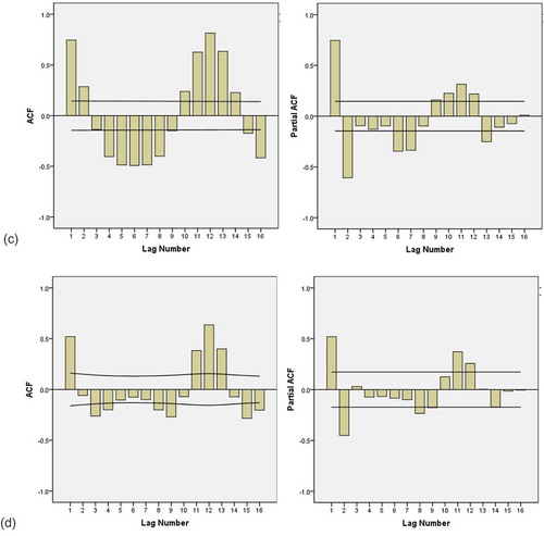
A fusion model based on the five ANN models described in Section 2 using snow cover and LAI data from MODIS products in addition to rainfall and runoff data was considered to predict the monthly reservoir inflow. The number of time delays for input parameters was extracted by ACF and partial ACF to determine the input combinations of the ANN models. The ACF, partial ACF and the corresponding 95% confidence bands from lags 0 to 16 were estimated for all input parameters; Figure 5 shows the lag-1 significant correlation for rainfall and runoff and lag-2 correlation coefficient for snow cover and LAI data used to describe the time-dependent variables. One set of antecedent rainfall and runoff values and two antecedent snow cover and LAI values were selected as inputs of the ANN models. Moreover, six input vectors, Q_t−1, P_t−1, S_t−1, S_t−2, LAI_t− and LAI_t−2 were selected to design the eight input combinations. The properties of input combinations are shown in Table 3.

Table 2. Different approaches of ANN models to forecasting the reservoir inflow.

Approach	Input combinations
1	$Q_t=f(P)$
2	$Q_t=f(P,Q)$
3	$Q_t=f(P,Q,S)$
4	$Q_t=f(P,Q,\mathrm{L}\mathrm{A}\mathrm{I})$
5	$Q_t=f(P,Q,S,\mathrm{L}\mathrm{A}\mathrm{I})$

Table 3. Properties of selected ANN models and input combinations.

		Number of neurons in hidden layers
		MLP				Spread
Approach	Model no.	First layer	Second layer	RBF	NARX	RBF	GRNN	Input combinations
1	1	4	4	3	15	5.07	29.04	$Q_t=f(P_{t-1})$
2	2	5	3	6	6	6.49	2.6	$Q_t=f(P_{t-1},Q_{t-1})$
3	3	4	2	8	4	7.05	3.35	$Q_t=f(P_{t-1},Q_{t-1},S_{t-1})$
	4	3	7	15	12	8.09	4.78	$Q_t=f(P_{t-1},Q_{t-1},S_{t-1},S_{t-2})$
4	5	3	9	5	12	12.6	4.9	$Q_t=f(P_{t-1},Q_{t-1},\mathrm{L}\mathrm{A}{\mathrm{I}}_{t-1})$
	6	5	4	7	15	1.22	4.35	$Q_t=f(P_{t-1},Q_{t-1},\mathrm{L}\mathrm{A}{\mathrm{I}}_{t-1},\mathrm{L}\mathrm{A}{\mathrm{I}}_{t-2})$
5	7	5	3	9	12	22.48	10.06	$Q_t=f(P_{t-1},Q_{t-1},S_{t-1},\mathrm{L}\mathrm{A}{\mathrm{I}}_{t-1})$
	8	5	4	10	17	4.44	4.35	$Q_t=f(P_{t-1},Q_{t-1},S_{t-1},S_{t-2},\mathrm{L}\mathrm{A}{\mathrm{I}}_{t-1},\mathrm{L}\mathrm{A}{\mathrm{I}}_{t-2})$

Figure 4. Selected datasets for (a) the training period and (b) the testing period.

Figure 5. ACF and partial ACF plots of (a) the runoff series, (b) the precipitation series, (c) the LAI series and (d) the snow cover series.

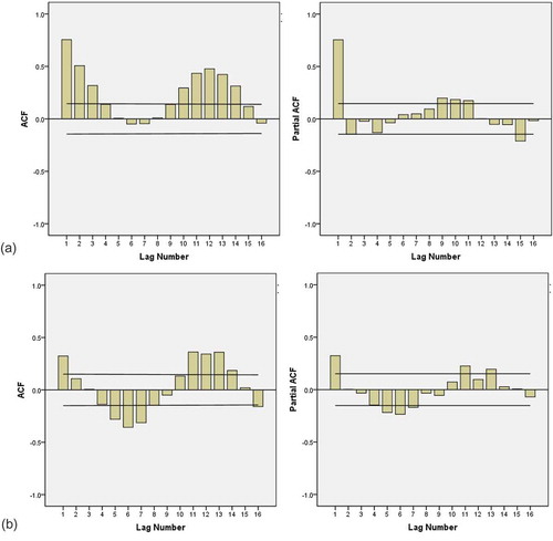
Figure 5. (Continued).

The optimal number of hidden layer neurons (for MLP1, MLP2, RBF and NARX models) and spread (for RBF and GRNN models) were obtained by the trial-and-error method according to the RMSE value in the test period. As an example for the MLP1 model, the effect of different numbers of neurons in the first hidden layer for the test period is presented in Figure 6, showing that the optimal number is 4 based on the lower RMSE values obtained.

Figure 6. Effect of number of neurons in the hidden layer on the RMSE value in the test period for Combination 1 in the MLP model.

The MLP1, MLP2 and NARX models were trained using five training algorithms (LM, BR, RP, SCG and GDX) for the hidden layer(s) and two activation functions – tangent-sigmoid (tansig) and log-sigmoid (logsig) – and the linear transfer function for the output layer were used. Based on the results of sensitivity analysis, the Levenberg-Marquardt and tangent-sigmoid have better performance than the other training algorithms and activation functions. These results are in agreement with those of Rezaeian Zadeh et al. (2010), who found the performance of the tangent-sigmoid activation function was better for the Khosroshirin basin (one of the sub-basins of the Mollasadra Dam’s basin). As an example, the results of eight combinations of the MLP1 model with various training algorithms and activation functions are shown in Table 4.

Table 4. Results of the MLP1 (MLP with one hidden layer) model for different training algorithms and activation functions. RMSE: root mean square error (10⁶ m³); r: correlation coefficient. LM: Levenberg-Marquardt; BR: Bayesian regularization; RP: resilient back-propagation; SCG: scaled conjugate gradient; and GDX: gradient descent with momentum and adaptive learning rate back-propagation.

				Training algorithm
Model no.	Architecture	Activation function	Statistical error index	LM	BR	RP	SCG	GDX
1	1-4-1	tansig	RMSE	16.28	49.8	49.8	49.4	50.8
			r	0.71	0.64	0.61	0.6	0.63
		logsig	RMSE	48.03	49.5	49.9	51.5	50.6
			r	0.61	0.63	0.63	0.61	0.65
2	2-5-1	tansig	RMSE	12.9	16.3	15.6	15.3	16.1
			r	0.83	0.83	0.7	0.8	0.84
		logsig	RMSE	14.6	15.2	15.2	15.8	18.6
			r	0.84	0.73	0.86	0.62	0.8
3	3-4-1	tansig	RMSE	9.66	13.1	15	15.1	16.4
			r	0.9	0.62	0.83	0.84	0.83
		logsig	RMSE	13.95	13.2	15	17.4	17.9
			r	0.92	0.6	0.79	0.88	0.81
4	4-3-1	tansig	RMSE	11.88	13.9	14.7	14.7	18.5
			r	0.84	0.67	0.87	0.87	0.76
		logsig	RMSE	15.71	14.4	15.2	16.3	18.9
			r	0.88	0.86	0.8	0.83	0.66
5	3-3-1	tansig	RMSE	10.28	12.8	15.3	15.4	17.1
			r	0.88	0.77	0.87	0.84	0.91
		logsig	RMSE	14.45	12.8	19.6	15.9	16.4
			r	0.92	0.75	0.86	0.84	0.87
6	4-5-1	tansig	RMSE	10.14	12.3	15.2	15	15.8
			r	0.9	0.79	0.91	0.86	0.86
		logsig	RMSE	12.97	12.4	16.8	14.9	16.2
			r	0.84	0.85	0.91	0.87	0.81
`7	4-5-1	tansig	RMSE	9.76	12.8	14.8	16.3	16.2
			r	0.9	0.88	0.84	0.85	0.85
		logsig	RMSE	14.59	12.8	15.8	16.6	16.1
			r	0.87	0.78	0.83	0.82	0.82
8	6-5-1	tansig	RMSE	9.6	13.9	16	14.8	18.6
			r	0.9	0.89	0.89	0.85	0.77
		logsig	RMSE	13.18	11.8	16.3	16.1	17.5
			r	0.8	0.87	0.83	0.86	0.69

The statistical error indices of the training and testing datasets for eight different input combinations of each ANN model were computed and are shown in Table 5. It can be seen from the results in Table 5 that the application of the rainfall data alone with short time series of rainfall (Combination 1) is inadequate to predict the runoff in the medium term (monthly). Also, the addition of other parameters into the input combinations can increase the accuracy of monthly reservoir inflow predictions. By comparing the results of combinations 1 and 2 (Table 5), it is found that using the runoff data in addition to rainfall data led to more accurate solutions. The results of models improved by various scenarios generated using snow cover, LAI, rainfall and runoff data are given in the combinations of models 3–8 (Table 5). For example, in the MLP1 model there is a decrease in RMSE and MAPE in the training and testing stages between combination 2 and combinations 3 and 4 (Table 5). Also in the MLP2 model, the values of RMSE and MAPE in the training and testing stages for combinations 3 and 4 are decreased compared with those for combination 2. The MLP2 model has a better prediction of monthly reservoir inflow compared with the MLP1 model in combinations 3 and 4 (Table 5). The results of combinations 5 and 6 indicate that using the LAI data can be helpful to better predict monthly reservoir inflow (compared with combination 2). Finally, based on Table 5, the use of both MODIS data (snow cover and LAI) in combinations 7 and 8 led to improved accuracy of the MLP models (compared with combination 2).The results of the RBF and GRNN models (Table5) are similar to those of the MLP1 and MLP2 models, so that using the same parameters of runoff, snow cover and LAI (one or a combination of these parameters) in addition to rainfall in the input combinations led to an increase in the accuracy and performance of the ANN models to predict monthly reservoir inflow.

Table 5. Results of the MLP1, MLP2, RBF, GRNN and NARX models for different input combinations.

		RMSE (10^6 m^3)		MAPE (%)		Willmott index		Correlation coefficient
Model no.	Architecture	Training	Testing	Training	Testing	Training	Testing	Training	Testing
MLP1 model
1	1-4-1	16.31	16.28	54.49	53.6	0.75	0.81	0.59	0.71
2	2-5-1	11.2	12.9	34.75	31.8	0.9	0.9	0.83	0.81
3	3-4-1	9.4	9.66	32.2	29.1	0.93	0.93	0.88	0.9
4	4-3-1	9.87	11.88	26.85	28.83	0.93	0.91	0.87	0.84
5	3-3-1	10.02	10.28	29.6	22.84	0.92	0.93	0.87	0.88
6	4-5-1	9.97	10.14	31.92	24	0.92	0.92	0.87	0.9
7	4-5-1	9.23	9.76	29.97	23.6	0.94	0.93	0.89	0.9
8	6-5-1	9.3	9.6	27.02	21.57	0.94	0.93	0.89	0.9
MLP2 model
1	1-4-4-1	16.36	14.68	52.62	59.85	0.73	0.86	0.6	0.75
2	2-5-3-1	9.68	11.9	26.56	31.13	0.93	0.92	0.88	0.86
3	3-4-2-1	9.34	10.13	30.6	26.7	0.94	0.93	0.88	0.89
4	4-3-7-1	9.56	9.66	26.51	25.51	0.93	0.93	0.88	0.92
5	3-3-9-1	9.16	10.8	28.95	28	0.94	0.91	0.89	0.89
6	4-5-4-1	9.07	9.77	33.47	22.76	0.94	0.95	0.9	0.89
7	4-5-3-1	8.77	8.67	28.53	24.75	0.94	0.95	0.9	0.93
8	6-5-4-1	9.47	10.08	26.49	23.84	0.94	0.93	0.88	0.88
RBF model
1	1-3-1	16.45	14.96	73.41	30.17	0.72	0.83	0.61	0.73
2	2-6-1	10.54	11.69	30.34	30.17	0.91	0.92	0.85	0.86
3	3-8-1	9.49	8.74	29.32	23.09	0.93	0.95	0.88	0.92
4	4-15-1	10.03	9.26	27.85	23.80	0.94	0.94	0.89	0.92
5	3-5-1	10.76	10.41	28.03	21.26	0.93	0.92	0.87	0.89
6	4-7-1	11.08	9.87	31.84	19.88	0.92	0.93	0.86	0.9
7	4-9-1	10.49	10.83	27.85	20.20	0.93	0.91	0.88	0.9
8	6-10-1	10.48	10.33	31.52	20.53	0.93	0.92	0.88	0.89
GRNN model
1	1-1-1	16.41	15.59	74.1	59.29	0.70	0.80	0.61	0.7
2	2-2-1	5.72	13.22	16.91	33.74	0.99	0.90	0.99	0.82
3	3-3-1	5.44	17.75	13.82	32.22	1.00	0.75	0.99	0.63
4	4-4-1	5.40	24.08	11.63	48.53	1.00	0.59	0.99	0.34
5	3-3-1	4.86	13.62	8.13	35.85	1.00	0.88	1.00	0.79
6	4-4-1	4.55	13.38	1.93	38.50	1.00	0.88	1.00	0.81
7	4-4-1	5.78	18.91	17.81	46.92	0.99	0.71	0.99	0.55
8	6-6-1	4.55	24.21	1.92	53.47	1.00	0.59	1.00	0.34
NARX model
1	1-15-1	13.8	14.96	63.68	62.39	0.83	0.85	0.73	0.73
2	2-6-1	9.82	10.44	42.19	35.84	0.92	0.93	0.88	0.88
3	3-4-1	8.96	9.72	37.55	28.6	0.93	0.93	0.9	0.9
4	4-12-1	5.29	12.6	23.15	33.43	0.92	0.9	0.96	0.82
5	3-12-1	7.12	12.48	27.77	28.7	0.91	0.9	0.93	0.83
6	4-15-1	7.48	11.94	29.5	34.47	0.92	0.91	0.93	0.85
7	4-12-1	5.67	13.12	26.51	26.85	0.92	0.9	0.96	0.81
8	6-17-1	6.14	9.93	31.29	35.15	0.91	0.92	0.95	0.9

The results of the NARX model (i.e. the dynamic ANN model tested) are also presented in Table 5. These results are similar to those of the static ANN models (MLP1, MLP2, RBF and GRNN) and the accuracy of predictions was increased by using the snow cover and LAI data in the input combinations.

It can be seen from Table 5 that combinations 3–8 have better prediction results in the different ANN models, but it is difficult to choose the best input combination and superior ANN model among all of them. Therefore, the Borda count method was used to rank the ANN model results, and the rankings of the combinations in each ANN model and among all ANN models are presented in Table 6. The results show that combinations 8, 7, 4, 6 and 3 have the highest B_i values and are selected as the best input combinations in the MLP1, MLP2, RBF, GRNN and NARX models, respectively. Based on these results, the GRNN and RBF models are found more accurate in the training and testing stages, respectively. Also, based on the results presented in Table 6, combination 7 (with Q_t−1, P_t−1, S_t−1 and LAI_t−1 as the input parameters) and the MLP2 model had the highest Borda value (B_i) among all the ANN models and these were selected as the best input combination and ANN model.

Table 6. Results of ranking the different input combinations in each and among all ANN models based on the Borda count method.

Network	Model no.	Borda Bi for in each ANN model	Rank in each ANN model	Borda Bi among all ANN models	Rank among all ANN models
MLP (with one hidden layer)	1	12	7	123	30
	2	20	6	168	27
	3	41	3	227	15
	4	37	5	216	19
	5	39	4	228	14
	6	37	5	219	17
	7	49	2	249	6
	8	54	1	264	2
MLP (with two hidden layers)	1	12	7	127	29
	2	26	6	211	21
	3	36	4	233	10
	4	41	3	252	4
	5	34	5	232	11
	6	41	3	238	6
	7	51	1	265	1
	8	42	2	250	5
RBF	1	10	7	122	31
	2	23	6	195	25
	3	47	2	254	3
	4	48	1	250	5
	5	34	5	230	12
	6	34	5	227	15
	7	39	3	233	10
	8	37	4	226	16
GRNN	1	24	8	115	32
	2	44	3	234	9
	3	37	4	217	18
	4	28	6	204	23
	5	46	2	233	10
	6	49	1	238	7
	7	25	7	200	24
	8	32	5	209	22
NARX	1	9	7	129	28
	2	29	6	194	26
	3	41	1	234	9
	4	38	4	229	13
	5	34	5	226	16
	6	34	5	215	20
	7	40	2	237	8
	8	39	3	228	14

Figures 7 and 8 show the scatter plots of observed versus predicted data of monthly reservoir inflow for the best combination of each ANN model (combinations 8, 7, 4, 6 and 3 in MLP1, MLP2, RBF, GRNN and NARX models, respectively) in the training and testing periods, respectively. Also, a comparison between observed and simulated values of monthly reservoir inflow for the best combination among all the ANN models in the training and testing periods are shown in Figure 9.

Figure 7. Scatter plots in the training period for the best input combination of the different ANN models.

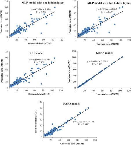
Figure 8. Scatter plots in the testing period for the best input combination of the different ANN models.

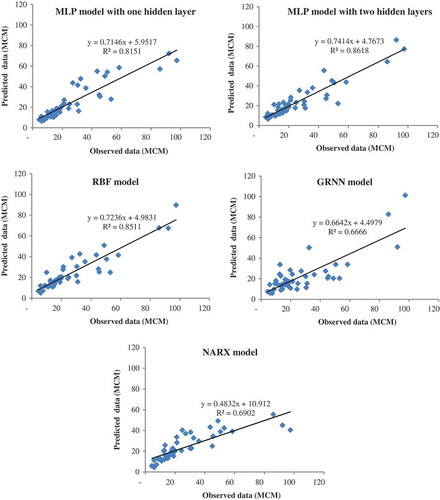
Figure 9. Comparison between observed and predicted runoff for the superior ANN model (combination 7 in MLP2): (a) training period and (b) testing period.

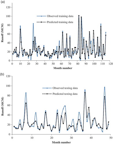
Figure 10. Scatter plots for the training and testing periods for the fusion-based neural network model.

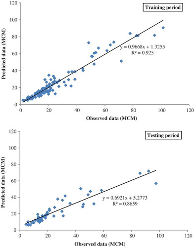
It should be noted that the simulated values have underestimated or overestimated low and high inflow rates and the model is unable to simulate these values accurately. This may be due to lack of a long-term series of data. Therefore, to receive a more accurate prediction of monthly reservoir runoff, a fusion-based neural network model was implemented using the MLP model with one hidden layer to combine the outputs of the best combination of individual ANN models, as shown in Table 6. The number of neurons in the hidden layer, the training algorithm and the activation function were determined similarly to the methodology described in Section 2.4.5. The results of sensitivity analysis showed that the Levenberg-Marquardt and tangent-sigmoid functions are the most suitable. The results of this fusion-based model are presented in Table 7. As shown in Table 7, the RMSE values of the fusion model in training and testing stages are 5.57 and 8.24 × 10⁶ m³, respectively, compared with 8.77 and 8.67 × 10⁶ m³ in training and testing stages, respectively, for the best combination among all the models (combination 7 of MLP2, Table 5). The MAPE values of the fusion model decreased to about 7.98 and 5.24% in the training and testing stages, respectively, compared to the best input combination among all the ANN models. The scatter plots of observed versus predicted data for monthly reservoir inflow for the fusion-based neural network model in the training and testing periods are shown in Figure 10.

Table 7. Results of the fusion-based neural network model in prediction of monthly reservoir inflow.

	RMSE (10^6 m^3)		MAPE (%)		Willmott index		Correlation coefficient
Architecture	Training	Testing	Training	Testing	Training	Testing	Training	Testing
5-5-1	5.57	8.24	20.55	19.51	0.99	0.98	0.96	0.94

4 Summary and conclusions

One of the main concerns in water resources planning and management is the selection of a simulation model to accurately predict reservoir inflow. Artificial neural networks (ANNs) are a type of data-driven model widely used in rainfall–runoff modelling. Recently, data and model fusion techniques to provide more accurate prediction and estimation have been successfully applied in many engineering fields, such as hydrological modelling. In this study, a new model fusion approach was developed using the best outputs of various individual ANN models. Five different types of ANN model were employed to predict the monthly runoff at the Mollasadra Dam, Fars Province, Iran. Since there is no sufficiently long time series of measured data (such as rainfall and runoff) in some watersheds, in this study, leaf area index (LAI) and snow cover data from MODIS in addition to in situ data (rainfall and runoff) from 2000 to 2015 were collected and processed by ENVI® and MATLAB® software before being used as input parameters of the ANN models. The same distribution of different flow regimes was obtained by the Levene test and the T test using training and testing datasets and different ANN models. The ACF and partial ACF were applied to determine the number of delays for each parameter and input combination. By considering five approaches, eight input combinations for the ANN models were identified. In approach 1 only the rainfall parameter and in approach 2 the rainfall and runoff parameters were used as input vectors. In approaches 3 and 4, snow cover and LAI, respectively, were added to the rainfall and runoff parameters. Finally, in approach 5, all four parameters were used. The accuracy of the models was evaluated using several statistical error indices. The Borda count method was used to rank the results of the different statistical error indices of the ANN models to determine the best input combination in each ANN model and the best overall ANN model. Finally, the fusion-based neural network model was developed by using the outputs of the best combination of different ANN models as inputs of the MLP model with one hidden layer. The results show that, in basins without long gauging records, just using the rainfall data (approach 1) to predict the monthly and annual runoff is insufficient, while using other parameters such as runoff in previous time steps can be effective. The performance of the ANN models was improved using the MODIS data (approaches 3, 4 and 5) in comparison to approach 2. Combination 7 (rainfall with one time lag, runoff with one time lag, snow cover with one time lag and LAI with one time lag as input parameters) and the MLP model with two hidden layers were selected as the best input combination and overall best model. According to the results of the fusion-based neural network model, the MAPE values were decreased compared to the best input combination in the superior model by about 7.98 and 5.24% in the training and testing stages, respectively.

The use of snow cover and LAI remote sensing data as hydrological model inputs in runoff prediction models has been limited and, so far, not used as ANN model inputs. However, hydrological modelling is complex because the rainfall–runoff phenomenon is influenced by many parameters, such as evaporation, infiltration, vegetation properties and variables of basin physiography. Considering all these parameters is very difficult, very expensive, time consuming, dependent on unavailable technologies, or the data are not available in some basins. Intelligent models such as ANNs do not consider the many complexities of systems and the simplicity of application of these models results in them being widely used.

Based on the above, the model fusion approach can lead to decreases in the prediction errors of ANN models in runoff modelling. Furthermore, MODIS products may be considered as input data to simulate monthly reservoir inflow as they are freely available for download. Finally, it should be mentioned that the proposed methodology was employed for one watershed and further studies must be performed for generalization of the results.

Disclosure statement

No potential conflict of interest was reported by the authors.

References

- Ababaei, B., et al., 2013. Reservoir daily inflow simulation using data fusion method. Irrigation and Drainage, 62 (4), 468–476.
- Abrahart, R.J. and See, L., 2002. Multi-model data fusion for river flow forecasting: an evaluation of six alternative methods based on two contrasting catchments. Hydrology and Earth System Sciences Discussions, 6 (4), 655–670. doi:10.5194/hess-6-655-2002
- Agarwal, A. and Singh, R.D., 2004. Runoff modelling through back propagation artificial neural network with variable rainfall–runoff data. Water Resources Management, 18 (3), 285–300. doi:10.1023/B:WARM.0000043134.76163.b9
- Albaradeyia, I., Hani, A., and Shahrour, I., 2011. WEPP and ANN models for simulating soil loss and runoff in a semi-arid Mediterranean region. Environmental Monitoring and Assessment, 180 (1), 537–556. doi:10.1007/s10661-010-1804-x
- Ang, M.R.C.O., Gonzalez, R.M., and Castro, P.P.M., 2014. Multiple data fusion for rainfall estimation using a NARX-based recurrent neural network – the development of the REIINN model. IOP Conference Series: Earth and Environmental Science, 17 (1), 012019. doi:10.1088/1755-1315/17/1/012019
- Aytek, A. and Alp, M., 2008. An application of artificial intelligence for rainfall-runoff modeling. Journal of Earth System Science, 117 (2), 145–155. doi:10.1007/s12040-008-0005-2
- Azmi, M., Araghinejad, S., and Kholghi, M., 2010. Multi model data fusion for hydrological forecasting using k-nearest neighbour method. Iranian Journal of Science and Technology, 34 (B1), 81.
- Balouchi, B., Nikoo, M.R., and Adamowski, J., 2015. Development of expert systems for the prediction of scour depth under live-bed conditions at river confluences: application of different types of ANNs and the M5P model tree. Applied Soft Computing, 34, 51–59. doi:10.1016/j.asoc.2015.04.040
- Bozorg-Haddad, O., et al., 2016. A self-tuning ANN model for simulation and forecasting of surface flows. Water Resources Management, 30 (9), 2907–2929. doi:10.1007/s11269-016-1301-2
- Chang, F.-J., et al., 2016. Prediction of monthly regional groundwater levels through hybrid soft-computing techniques. Journal of Hydrology, 541, 965–976. doi:10.1016/j.jhydrol.2016.08.006
- Chang, F.-J., et al., 2015. Modeling water quality in an urban river using hydrological factors – data driven approaches. Journal of Environmental Management, 151, 87–96. doi:10.1016/j.jenvman.2014.12.014
- Cheng, C.-T., et al., 2015. Daily reservoir runoff forecasting method using artificial neural network based on quantum-behaved particle swarm optimization. Water, 7 (12), 4232–4246. doi:10.3390/w7084232
- Cigizoglu, H.K. and Alp, M., 2004. Rainfall-runoff modelling using three neural network methods. In: L. Rutkowski, et al., ed. Artificial Intelligence and Soft Computing - ICAISC 2004: 7th International Conference, Zakopane, Poland. 7–11 June 2004. Proceedings. Berlin, Heidelberg: Springer Berlin Heidelberg, 166–171.
- Conesa-Garcia, C., et al., 2010. Hydraulic geometry, gis and remote sensing, techniques against rainfall-runoff models for estimating flood magnitude in ephemeral fluvial systems. Remote Sensing, 2 (11), 2607–2628. doi:10.3390/rs2112607
- Corona, J.A.I., et al., 2014. Remote sensing and ground-based weather forcing data analysis for streamflow simulation. Hydrology, 1 (1), 89–111. doi:10.3390/hydrology1010089
- Daofeng, L., et al., 2004. Impact of land-cover and climate changes on runoff of the source regions of the Yellow River. Journal of Geographical Sciences, 14 (3), 330–338. doi:10.1007/BF02837414
- Dar, L.A., 2017. Rainfall–runoff modeling using artificial neural network. International Research Journal of Engineering and Technology, 4 (11), 424–427.
- Dhamge, N.R., Atmapoojya, S.L., and Kadu, M.S., 2012. Genetic algorithm driven ANN model for runoff estimation. Procedia Technology, 6, 501–508. doi:10.1016/j.protcy.2012.10.060
- Diaconescu, E., 2008. The use of NARX neural networks to predict chaotic time series. Wseas Transactions on Computer Research, 3 (3), 182–191.
- Engman, E.T., 1997. Soil moisture, the hydrologic interface between surface and ground waters. Iahs Publication, 129–140.
- Fitch, D.T., et al., 2010. MODIS vegetation metrics as indicators of hydrological response in watersheds of California Mediterranean-type climate zones. Remote Sensing of Environment, 114 (11), 2513–2523. doi:10.1016/j.rse.2010.05.026
- Garcia-Quijano, J.F. and Barros, A.P., 2005. Incorporating canopy physiology into a hydrological model: photosynthesis, dynamic respiration, and stomatal sensitivity. Ecological Modelling, 185 (1), 29–49. doi:10.1016/j.ecolmodel.2004.08.024
- Georgievsky, M.V., 2009. Application of the Snowmelt Runoff model in the Kuban river basin using MODIS satellite images. Environmental Research Letters, 4 (4), 045017. doi:10.1088/1748-9326/4/4/045017
- Ghazali, M., Honar, T., and Nikoo, M.R., 2018. A hybrid TOPSIS-agent-based framework for reducing the water demand requested by stakeholders with considering the agents’ characteristics and optimization of cropping pattern. Agricultural Water Management, 199, 71–85. doi:10.1016/j.agwat.2017.12.014
- Gigante, V., et al., 2009. Influences of leaf area index estimations on water balance modeling in a Mediterranean semi-arid basin. Natural Hazards and Earth System Sciences, 9 (3), 979–991. doi:10.5194/nhess-9-979-2009
- Gowda, C.C. and Mayya, S.G., 2014. Rainfall runoff modelling using generalized neural network and radial basis network. International Journal of Intelligent Systems and Applications in Engineering, 2 (4), 76–79. doi:10.18201/ijisae.82758
- Guzman, S.M., Paz, J.O., and Tagert, M.L.M., 2017. The use of NARX neural networks to forecast daily groundwater levels. Water Resources Management, 31 (5), 1591–1603. doi:10.1007/s11269-017-1598-5
- Hadiani, S. and Hadiani, R., 2015. Analysis of Rainfall-runoff neuron input model with artificial neural network for simulation for availability of discharge at Bah Bolon Watershed. Procedia Engineering, 125, 150–157. doi:10.1016/j.proeng.2015.11.022
- Huang, S., et al., 2015. Identification of abrupt changes of the relationship between rainfall and runoff in the Wei River Basin, China. Theoretical and Applied Climatology, 120 (1), 299–310. doi:10.1007/s00704-014-1170-7
- Irfan, M., et al., 2016. Geographical general regression neural network (GGRNN) tool for geographically weighted regression analysis. Geoprocessing, 24, 154–159.
- Islam, M., et al., 2001. Forecasting of river flow data with a general regression neural network. Iahs Publication, 272, 285–290.
- Jain, A., Sudheer, K.P., and Srinivasulu, S., 2004. Identification of physical processes inherent in artificial neural network rainfall runoff models. Hydrological Processes, 18 (3), 571–581. doi:10.1002/(ISSN)1099-1085
- Jayawardena, A. and Fernando, D.A.K., 1998. Use of radial basis function type artificial neural networks for runoff simulation. Computer‐Aided Civil and Infrastructure Engineering, 13 (2), 91–99. doi:10.1111/0885-9507.00089
- Jothiprakash, V. and Magar, R.B., 2012. Multi-time-step ahead daily and hourly intermittent reservoir inflow prediction by artificial intelligent techniques using lumped and distributed data. Journal of Hydrology, 450–451, 293–307. doi:10.1016/j.jhydrol.2012.04.045
- Khaleghi, B., et al., 2013. Multisensor data fusion: A review of the state-of-the-art. Information Fusion, 14 (1), 28–44. doi:10.1016/j.inffus.2011.08.001
- Kumar, S., et al., 2015. Reservoir inflow forecasting using ensemble models based on neural networks, wavelet analysis and bootstrap method. Water Resources Management, 29 (13), 4863–4883. doi:10.1007/s11269-015-1095-7
- Lai, X., et al., 2014. Variational assimilation of remotely sensed flood extents using a 2-D flood model. Hydrology and Earth System Sciences, 18 (11), 4325–4339. doi:10.5194/hess-18-4325-2014
- Lee, S.C., Lin, H.T., and Yang, T.Y., 2010. Artificial neural network analysis for reliability prediction of regional runoff utilization. Environmental Monitoring and Assessment, 161 (1), 315–326. doi:10.1007/s10661-009-0748-5
- Lee, W.-K. and Tuan Resdi, T.A., 2016. Simultaneous hydrological prediction at multiple gauging stations using the NARX network for Kemaman catchment, Terengganu, Malaysia. Hydrological Sciences Journal, 61 (16), 2930–2945. doi:10.1080/02626667.2016.1174333
- Leontaritis, I.J. and Billings, S.A., 1985. Input-output parametric models for non-linear systems Part II: stochastic non-linear systems. International Journal of Control, 41 (2), 329–344. doi:10.1080/0020718508961130
- Li, H., et al., 2009. Predicting runoff in ungauged catchments by using Xinanjiang model with MODIS leaf area index. Journal of Hydrology, 370 (1–4), 155–162. doi:10.1016/j.jhydrol.2009.03.003
- Lin, G.-F. and Chen, L.-H., 2004. A non-linear rainfall-runoff model using radial basis function network. Journal of Hydrology, 289 (1), 1–8. doi:10.1016/j.jhydrol.2003.10.015
- Mahmoud, S.H., 2014. Investigation of rainfall–runoff modeling for Egypt by using remote sensing and GIS integration. CATENA, 120, 111–121. doi:10.1016/j.catena.2014.04.011
- Meng, X., et al., 2015. A threshold artificial neural network model for improving runoff prediction in a karst watershed. Environmental Earth Sciences, 74 (6), 5039–5048. doi:10.1007/s12665-015-4562-9
- Michailovsky, C.I. and Bauer-Gottwein, P., 2014. Operational reservoir inflow forecasting with radar altimetry: the Zambezi case study. Hydrology and Earth System Sciences, 18 (3), 997–1007. doi:10.5194/hess-18-997-2014
- Milewski, A., et al., 2009. A remote sensing solution for estimating runoff and recharge in arid environments. Journal of Hydrology, 373 (1–2), 1–14. doi:10.1016/j.jhydrol.2009.04.002
- Mishra, S., et al., 2014. An efficient approach of artificial neural network in runoff forecasting. International Journal of Computer Applications, 92 (5), 9–15. doi:10.5120/16003-4991
- Modaresi, F., Araghinejad, S., and Ebrahimi, K., 2017. A comparative assessment of artificial neural network, generalized regression neural network, least-square support vector regression, and K-nearest neighbor regression for monthly streamflow forecasting in linear and nonlinear conditions. Water Resources Management, 32 (1), 243–258.
- Mondal, S.K., et al., 2012. A comparative study for prediction of direct runoff for a river basin using geomorphological approach and artificial neural networks. Applied Water Science, 2 (1), 1–13. doi:10.1007/s13201-011-0020-3
- Nafarzadegan, A.R., et al., 2018. Socially-optimal and nash pareto-based alternatives for water allocation under uncertainty: an approach and application. Water Resources Management, 32 (9), 2985–3000. doi:10.1007/s11269-018-1969-6
- Nagler, T., et al., 2008. Assimilation of meteorological and remote sensing data for snowmelt runoff forecasting. Remote Sensing of Environment, 112 (4), 1408–1420. doi:10.1016/j.rse.2007.07.006
- Nanda, T., et al., 2016. A wavelet-based non-linear autoregressive with exogenous inputs (WNARX) dynamic neural network model for real-time flood forecasting using satellite-based rainfall products. Journal of Hydrology, 539, 57–73. doi:10.1016/j.jhydrol.2016.05.014
- Nigam, R., Nigam, S., and Mittal, S.K., 2014. Stochastic modelling of rainfall and runoff phenomenon: a time series approach review. International Journal of Hydrology Science and Technology, 4 (2), 81–109. doi:10.1504/IJHST.2014.066437
- Nourani, V., Komasi, M., and Mano, A., 2009. A multivariate ANN-wavelet approach for rainfall-runoff modeling. Water Resources Management, 23 (14), 2877–2894. doi:10.1007/s11269-009-9414-5
- Okkan, U., 2012. Wavelet neural network model for reservoir inflow prediction. Scientia Iranica, 19 (6), 1445–1455. doi:10.1016/j.scient.2012.10.009
- Omidvar, K., Nabavizadeh, M., and Samarehghasem, M., 2015. assessment of NARX neural network in prediction of daily precipitation in Kerman province. Journal of Physical Geograohy, 8 (27), 73–89.
- Piotrowski, A.P., et al., 2016. On the importance of training methods and ensemble aggregation for runoff prediction by means of artificial neural networks. Hydrological Sciences Journal, 61 (10), 1903–1925.
- Rajurkar, M.P., Kothyari, U.C., and Chaube, U.C., 2004. Modeling of the daily rainfall-runoff relationship with artificial neural network. Journal of Hydrology, 285 (1–4), 96–113. doi:10.1016/j.jhydrol.2003.08.011
- Reshma, T., et al., 2010. Simulation of runoff in watersheds using SCS-CN and muskingum-cunge methods using remote sensing and geographical information systems. International Journal of Advanced Science and Technology, 25, 31–42.
- Rezaeian Zadeh, M., et al., 2010. Daily outflow prediction by multi layer perceptron with logistic sigmoid and tangent sigmoid activation functions. Water Resources Management, 24 (11), 2673–2688. doi:10.1007/s11269-009-9573-4
- Rezaeianzadeh, M., Stein, A., and Cox, J.P., 2016. Drought forecasting using markov chain model and artificial neural networks. Water Resources Management, 30 (7), 2245–2259. doi:10.1007/s11269-016-1283-0
- Rezaeianzadeh, M., et al., 2013. Assessment of a conceptual hydrological model and artificial neural networks for daily outflows forecasting. International Journal of Environmental Science and Technology, 10 (6), 1181–1192. doi:10.1007/s13762-013-0209-0
- Riad, S., et al., 2004. Rainfall-runoff model usingan artificial neural network approach. Mathematical and Computer Modelling, 40 (7), 839–846. doi:10.1016/j.mcm.2004.10.012
- Roy, A., Royer, A., and Turcotte, R., 2010. Improvement of springtime streamflow simulations in a boreal environment by incorporating snow-covered area derived from remote sensing data. Journal of Hydrology, 390 (1–2), 35–44. doi:10.1016/j.jhydrol.2010.06.027
- Ruslan, F.A., et al., 2013. Flood prediction using NARX neural network and EKF prediction technique: A comparative study. In: 2013 IEEE 3rd International Conference on System Engineering and Technology, 19–20 August 2013, Shah Alam, Malaysia, 203–208.
- Sahin, F., 1997. A radial basis function approach to a color image classification problem in a real time industrial application. Doctoral dissertation, Virginia Tech.
- Samanta, S., 2015. Geospatial data for surface runoff and transport capacity modeling. International Journal of Remote Sensing and Geoscience, 4 (1), 91–100.
- Sarmiento, C.J.S., Gonzalez, R.M., and Castro, P.P.M., 2012. Reservoir Inflow Estimation Using Remote Sensing, GIS and Geosimulation. Journal of Earth Science and Engineering, 2 (8), 472.
- Senthil Kumar, A., et al., 2005. Rainfall-runoff modelling using artificial neural networks: comparison of network types. Hydrological Processes, 19 (6), 1277–1291. doi:10.1002/(ISSN)1099-1085
- Sharma, S. and Tiwari, K., 2009. Bootstrap based artificial neural network (BANN) analysis for hierarchical prediction of monthly runoff in Upper Damodar Valley Catchment. Journal of Hydrology, 374 (3), 209–222. doi:10.1016/j.jhydrol.2009.06.003
- Shiau, J.-T. and Hsu, H.-T., 2016. Suitability of ANN-based daily streamflow extension models: a case study of Gaoping River basin, Taiwan. Water Resources Management, 30 (4), 1499–1513. doi:10.1007/s11269-016-1235-8
- Shrivastava, P., Tripathi, M., and Das, S., 2004. Hydrological modelling of a small watershed using satellite data and gis technique. Journal of the Indian Society of Remote Sensing, 32 (2), 145–157. doi:10.1007/BF03030871
- Siou, L.K.A., et al., 2012. Optimization of the generalization capability for rainfall–runoff modeling by neural networks: the case of the Lez aquifer (southern France). Environmental Earth Sciences, 65 (8), 2365–2375. doi:10.1007/s12665-011-1450-9
- Specht, D.F., 1991. A general regression neural network. IEEE Transactions on Neural Networks, 2 (6), 568–576. doi:10.1109/72.97934
- Srinivasulu, S. and Jain, A., 2006. A comparative analysis of training methods for artificial neural network rainfall–runoff models. Applied Soft Computing, 6 (3), 295–306. doi:10.1016/j.asoc.2005.02.002
- Tayyab, M., et al., 2016. Streamflow prediction by applying generalized regression network with time series decomposition method. Indonesian Journal of Electrical Engineering and Computer Science, 4 (3), 611–616. doi:10.11591/ijeecs.v4.i3.pp611-616
- Valipour, M., Banihabib, M.E., and Behbahani, S. M. R, 2013. Comparison of the ARMA, ARIMA, and the autoregressive artificial neural network models in forecasting the monthly inflow of Dez dam reservoir. Journal of Hydrology, 476, 433–441. doi:10.1016/j.jhydrol.2012.11.017
- Wang, W., Jin, J., and Li, Y., 2009. Prediction of inflow at three gorges dam in Yangtze River with wavelet network model. Water Resources Management, 23 (13), 2791–2803. doi:10.1007/s11269-009-9409-2
- Yildiz, O. and Barros, A.P., 2007. Elucidating vegetation controls on the hydroclimatology of a mid-latitude basin. Journal of Hydrology, 333 (2), 431–448. doi:10.1016/j.jhydrol.2006.09.010
- Yin, S., et al., 2016. A combined rotated general regression neural network method for river flow forecasting. Hydrological Sciences Journal, 61 (4), 669–682. doi:10.1080/02626667.2014.944525
- Zeroual, A., Meddi, M., and Assani, A.A., 2016. Artificial neural network rainfall-discharge model assessment under rating curve uncertainty and monthly discharge volume predictions. Water Resources Management, 30 (9), 3191–3205. doi:10.1007/s11269-016-1340-8
- Zhang, Y., et al., 2008. Estimating catchment evaporation and runoff using MODIS leaf area index and the Penman-Monteith equation. Water Resources Research, 44 (10). doi:10.1029/2007WR006563
- Zhang, Y., 2010. Using long term water balances to parameterize surface conductances and calculate evaporation at 0.05 spatial resolution. Water Resources Research, 46 (5). doi:10.1029/2009WR008716
- Zhang, Y., et al., 2011. Incorporating vegetation time series to improve rainfall-runoff model predictions in gauged and ungauged catchments. In: Modelling and Simulation Society of Australian and New Zealand. Presented at the MODSIM 2011 International Congress on Modelling and Simulation. Perth, Australia, 3455–3461.
- Zhou, Y., et al., 2013. Improving runoff estimates using remote sensing vegetation data for bushfire impacted catchments. Agricultural and Forest Meteorology, 182, 332–341. doi:10.1016/j.agrformet.2013.04.018