Beerkan multi-runs for characterizing water infiltration and spatial variability of soil hydraulic properties across scales

ABSTRACT

A method is presented for characterizing the spatial variability of water infiltration and soil hydraulic properties at the transect and field scales. The method involves monitoring a set of 10 Beerkan runs distributed over a 1-m length of soil, and running BEST (Beerkan estimation of soil transfer parameters) methods to derive hydraulic parameters. The Beerkan multi-runs (BMR) method provides a significant amount of data at the transect scale, allowing the determination of correlations between water infiltration variables and hydraulic parameters, and the detection of specific runs affected by preferential flow or water repellence. The realization of several BMRs at several transects on the same site allows comparison of the variation between locations (spatial variability at the field scale) and at the transect scale (spatial variability at the metre scale), using analysis of variance. From the results, we determined the spatial variability of water infiltration and hydraulic parameters as well as its characteristic scale (transect versus field).

KEYWORDS:

• beerkan
• multi-runs
• BEST methods
• spatial variability
• transect scale
• field scale

Editor S. Archfield Associate editor F. Tauro

Introduction

Knowledge of the water budget in the vadose zone is a prerequisite for the optimum management of water resources and the quality of soil (Haverkamp et al. 2006). Soil is the location in which water infiltration and groundwater recharge occur. Also, soil ensures the filtration of pollutants carried by infiltrating water, and thus offers an eco-service by filtering water before it reaches the groundwater (Bouwer 2002, Hatt et al. 2009). The hydraulic characterization of soil has been the focus of intensive research for many decades (Angulo-Jaramillo et al. 2016). Several methods have been developed to characterize the two main properties of soil, namely its capability to store water by capillarity and its capability to let water flow through it. The water-retention curve and hydraulic conductivity have been the target of many experimental methods and protocols (Angulo-Jaramillo et al. 2016).

Of the large number of methods that are available for the characterization of soil hydraulic properties, the Beerkan estimation of soil transfer parameters (BEST) methods were developed to provide the whole set of hydraulic parameters and the complete determination of soil hydraulic curves (Lassabatere et al. 2006, Yilmaz et al. 2010, Bagarello et al. 2014). These methods rely on the Beerkan method, which was pioneered by Braud et al. (2005), and which involves infiltrating several known volumes of water through a single ring installed on the ground. The Beerkan method permits the quantification of the cumulative infiltration obtained at a quasi-zero water-pressure head, and can be considered as a simplified type of tension infiltrometer with tension equal to zero. The combination of the Beerkan protocol and BEST methods has been used extensively for many applications, including the characterization of agricultural soils (e.g. Bagarello and Iovino 2012, Alagna et al. 2016), forest soils (e.g. Siltecho et al. 2015, Di Prima et al. 2017) and anthropic and urban soils (e.g. Lassabatere et al. 2010, Yilmaz et al. 2010, 2016). These methods have become quite popular because of their ease, low cost and the completeness of the hydraulic characterization (Lassabatere et al. 2009). However, some questions remain regarding how representative the BEST results are, in particular given the spatial variability of hydraulic properties and water infiltration at the field scale. In most studies, few experiments were performed assuming that the soil is uniform, and that water infiltration is necessarily uniform. The proposed estimated water retention or hydraulic functions are often based on a small number of samples, often three replicates (e.g. Cannavo et al. 2010, Lassabatere et al. 2010). Also, experiments are often performed as a function of soil texture and structure variability (e.g. Goutaland et al. 2013), but the variability of the response for the same soil texture and structure is not considered. In addition, any Beerkan run may be influenced by preferential flow (Lassabatere et al. 2014). The lack of replication close to the same place limits the awareness of the potential sampling of the macropore network and the related activation of the preferential flow. Additional data are needed to eliminate erroneous tests or runs that are impacted by preferential flow.

In this study, we developed a Beerkan multi-runs (BMR) procedure for the simultaneous application of a set of 10 Beerkan experiments with rings aligned along a 1-m-long transect above the soil surface. The rings are monitored simultaneously, leading to a set of 10 water infiltration experiments and related sets of hydraulic parameters after modelling with BEST methods. At the local scale, the BMR procedure is first expected to give insight into the potential preferential flow or flow impedance by water repellency along the transect. Contrasting behaviours between runs may indicate the occurrence of such specific flows. Secondly, a set of 10 cumulative infiltrations and related sets of estimated hydraulic parameters can be considered appropriate for statistical analysis. Such sets enable the accurate estimation of the mean trends, together with the spread around the means, and how to relate cumulative infiltration to the soil hydraulic parameters combined with additional observations to identify processes at the transect scale (root network, hydrophobicity, etc.). In addition to the gains at this scale, the BMR approach may be carried out at several places in the field to test the influence of any factor expressing at larger scales, such as the type of soil, the effect of tree or plant proximity, soil cultivation and fires. The significant amount of data produced with 10 sets of data per experimental location strengthens the statistical comparison of the results between the different transects at different places, which permits the statement of conclusions in the situation where a single datum per location would have been insufficient.

Material and methods

BMR experimental protocol

Three 1-m-long transects were drawn on randomly selected locations within the study site (Fig. 1(a)). Along these transects, the superficial herbaceous vegetation was carefully cut, without causing any disturbance to the root system. The first layer was removed if necessary (leaves and detritus). For each transect, 10 rings that were 5 cm in diameter were spaced out at equal distances of 5 cm and inserted into the soil to prevent any water leakage. Close to each transect, an undisturbed area of soil was sampled to determine the bulk density. The soil porosity was then determined from the dry bulk density, and the mineral density measured on the soil particle. Other soil volumes were sampled to determine the initial water content and the particle-size distribution. Several 17-mL volumes of water were prepared, to be poured into the rings. Cumulative infiltration, I(t) [L], is defined by the total infiltration height (cumulative infiltrated volume divided by the ring surface) as a function of total infiltration time. For each transect, the infiltration experiments were carried out simultaneously, and were started by pouring into each cylinder the first volume of water, while recording the time needed for complete infiltration. When the amount of water had completely infiltrated into a particular cylinder, another identical volume was quickly poured. This procedure was repeated 15 times for each run and, in all cases, until the differences in infiltration times between consecutive trials became negligible. Finally, soil samples were taken for the determination of the final water contents. Even if the monitoring of a set of 10 Beerkan runs at the same time may appear excessive, the experiment was shown to be feasible, and is schematically illustrated in Figure 1(b).

Figure 1. Field experimental set-up of the Beerkan multi-runs (BMR) procedure: (a) BMR test over a grass soil; (b) schematic chart of the methodology; (c) water repellency at the site; and (d) infiltration bulbs at the end of the experiments for transect Tr 2.

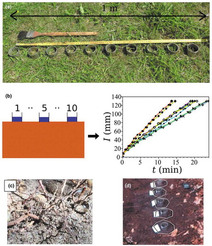
The site is located in the gardens at Wageningen University, the Netherlands. The soil is a loamy sand (Table 1). Three different transect locations were selected at the same site. These transects were selected such that they have different soil structure and proximity to trees, i.e. two Quercus and one Fagus. The measurements of initial water and bulk density were determined for several samples over the site. The particle-size distribution, bulk density and water contents were homogeneous at the field scale. Consequently, averages were assigned to all of the Beerkan runs, regardless of the position in the transect or the location of the transect in the field.

Table 1. Coordinates of the experimental site (Forest), clay, silt and sand content (US Department of Agriculture classification system), soil textural classification, dry-soil bulk density (ρ_b), initial volumetric soil-water content (θ₀) and saturated volumetric water content (θ_s). Standard deviations are indicated in parentheses.

Variable	Value
Coordinates	51°58ʹ52.3ʺN
	5°39ʹ43.1ʺE
Clay (%)	8.32 (2.67)
Silt (%)	9.66 (0.54)
Sand (%)	82.0 (2.26)
Textural classification	Loamy sand
ρb (g cm^−3)	0.972 (0.18)
θ0 (cm^3 cm^−3)	0.161 (0.10)
θs (cm^3 cm^−3)	0.634 (0.06)

We also computed the averaged infiltration rate, IR [L T⁻¹], which corresponds to the total cumulative infiltration divided by the total infiltration time, and the depth of wetting front for all infiltration experiments at a given time of 10 min, Z_wf [L]. For this purpose, we considered a piston-flow width displacement of the volume of water in the soil porosity, leading to the following equation:

(1) $Z_{\mathrm{w}\mathrm{f}}=\frac{I\left(t\right)}{\left({\theta }_f-{\theta }_i\right)}$(1)

where θ_f [L³ L⁻³] and θ_i [L³ L⁻³] are the final and initial water contents, respectively. The final water content was equal to the soil porosity. The parameters IR and Z_wf are quantitative indicators of water infiltration, and are much easier to compare than curves. These two variables were compared between runs for the same transect (transect scale) and between transects (field scale).

BEST analysis and statistical analysis

Each cumulative infiltration was treated using the three BEST methods (Slope, Intercept and Steady-state), which were developed respectively by Lassabatere et al. (2006), Yilmaz et al. (2010) and Bagarello et al. (2014). These methods consider that the water-retention function is described by the van Genuchten model (1980) along with Burdine’s condition (m = 1 − 2/n), and the hydraulic conductivity is described by the Brooks and Corey (1964) relationship, with the exponent η = 2/(m n) + 3 (Lassabatere et al. 2006). The three methods consider that the residual water content is zero, and that the saturated water content equals the soil porosity. The three methods treat the particle-size distribution with the pedotransfer functions (PTFs) developed in Lassabatere et al. (2006) to derive the shape parameters n, m and η. Then, the three models utilize infiltration data to derive the soil sorptivity, S [L T^−0.5] and the saturated soil hydraulic conductivity, K_s [L T⁻¹], before deriving the scale parameter for the water-pressure head, h_g [L]. The difference between the three methods involves their approaches to fitting the experimental cumulative infiltration to the approximate expansion for transient and steady states defined by Haverkamp et al. (1994), as well as to deriving S, K_s and h_g. More specifically, BEST-Slope uses the slope of the straight line defined by the last points (representative of the steady state) to link S and K_s, before fitting the transient model to the experimental data by the sole optimization of S. BEST-Intercept uses the intercept of the straight line defined by the last points to relate S and K_s, before fitting the transient model to the experimental data by the optimization of S. Finally, BEST-Steady-state uses both the intercept and the slope of the straight line defined by the last points to resolve a set of two equations (Di Prima et al. 2016), leading to the estimation of the two unknowns. Once S and K_s are determined, h_g can be derived as described in Lassabatere et al. (2006). The different structures of the three BEST methods make them sensitive to different kinds of input errors (e.g. Di Prima et al. 2016). With real data, it is then recommended that the three methods be run and their estimates combined. More details on their design and application may be found in Angulo-Jaramillo et al. (2016).

From a statistical perspective, we verified that the estimates for the scale parameter for water pressure h_g and the saturated hydraulic conductivity K_s were normally distributed, using the QQ plot and the Kolmogorov-Smirnov test (R Core Team 2013). Then, for each run, the values of the parameters were estimated by considering the arithmetic average of the three different estimates obtained with the BEST-Slope, BEST-Intercept and BEST-Steady-state methods. Linear models were used to test the correlation between variables, and in particular IR and Z_wf, on the one hand, and the hydraulic parameters, on the other. We also used the one-way ANalysis Of VAriance (ANOVA) to test the significance of the differences between the three locations compared with the variability obtained per the Beerkan multi-run. The ANOVA splits the variance of a particular observed variable into components that are attributable to different sources of variation, including explicative variables and the residual errors. The ANOVA compares the different components and reports the significance of the contribution of the compartments related to the explicative variables to the total variance. The one-way ANOVA considers only one explicative variable, whereas more complex ANOVAs (two ways and even more) may consider a larger number of explicative variables. In this study, the explicative variable is the location of the transects, and the ANOVA is thus one-way. The graphs and the statistics were carried out using the free software Scilab (Campbell et al. 2010) and R (R Core Team 2013).

Results

Three examples of Beerkan multi-runs

The three BMR experiments are depicted in Fig. 2, with the cumulative infiltrations (Fig. 2(a), (d) and (g)), the infiltration rates (Fig. 2(b), (e) and (h)) and the depths of the wetting fronts Z_wf (Fig. 2(c), (f) and (i)). The infiltration rates were obtained by differentiating the cumulative infiltrations, i.e. q = ΔI/Δt, and the values of Z_wf were obtained using Equation (1), considering the cumulative infiltration after 10 min.

Figure 2. (a, d, g) Cumulative infiltrations, (b, e, h) infiltration rates, and (c, f, i) estimated wetting-front positions for transects Tr 1, Tr 2 and Tr 3.

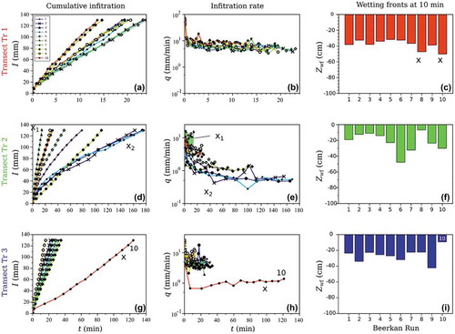
For transect Tr 1, the cumulative infiltrations have similar shapes, with a concave part at the beginning followed by a more linear part (Fig. 2(a)). The infiltration rates show a decreasing part, corresponding to the concave part of cumulative infiltrations, before stabilizing and delineating a plateau (Fig. 2(b)). The wetting fronts are quite uniform, with similar values over the transect (Fig. 2(c)). The deepest wetting fronts correspond to the rings with the highest values of IR. We note deeper wetting fronts and higher infiltration rates at the rings numbered 8–10 (Fig. 2(c), denoted by x).

For transect Tr 2, the variability between cumulative infiltrations is much more pronounced (Fig. 2(d)). Some of the curves have a linear part with a steep slope (Fig. 2(d), denoted by x₁). In contrast, others may exhibit a very concave shape, without any linear part (Fig. 2(d), x₂). These differences in terms of shape may be related to infiltration rates (Fig. 2(e)), with a quick stabilization of infiltration rate at high values for the linear cumulative infiltrations (Fig. 2(e), x₁) and, conversely, continuously decreasing infiltration rate for the concave cumulative infiltrations (Fig. 2(e), x₂). Compared with transect Tr 1, the distribution of wetting front depths is more uneven, with more important infiltration at rings 5–7, in the centre of the transect, and rings 9–10 at the right edge, and with lower infiltration at the left edge.

For transect Tr 3, the beam of cumulative infiltration is comparable to that of transect Tr 1 (Fig. 2(a)), except that run 10 behaves as an outlier (Fig. 2(g), x). This outlier is characterized by a concave shape, followed successively by a linear part, and a final slightly convex line (Fig. 2(g), x). The related infiltration rate shows a decreasing part, followed by a constant increase (Fig. 2(h), x). Such a pattern is typical for water repellency, when water infiltration is impeded at the beginning owing to a soil that is too dry (Lassabatere et al. 2013). The distribution of wetting fronts is quite even, except for run 10, with a very low depth relative to the water repellency (Fig. 2(i)). There was no visual evidence for any physical factor to explain the water repellency observed for run 10. A higher organic matter content may be expected locally. However, very water-repellent conditions may be obtained at the site (Fig. 1(c)).

It is clear that BMR experiments are very informative. For each transect, the experimental data encompass a set of 10 datasets (cumulative infiltration, infiltration rate, wetting front depth), which allows a more appropriate description of the average response of the soil, the dispersion around the average response, and the potential identification of outliers. These data are statistically sound, and give sufficient information to conclude about the spatial variability obtained at the transect scale.

The distribution of wetting fronts provides further information because it maps the spatial variability of the soil response at the transect scale (Fig. 2(c), (f) and (i)). These distributions may be considered as a good indicator of the wetting front that would have been obtained with a rainfall simulator, but with less intensive work and devices (Di Prima et al. 2017). The transects Tr 1 and Tr 3 did not show any particular spatial pattern, whereas Tr 2 exhibited higher infiltration rates in the centre and at the right edge of the transect. However, there was no clear explanation in terms of soil texture and structure for such a gradient between the left edge and the rest of the transects. Visual observations confirmed no particular change along the transect in terms of soil texture or structure. A subsequent study will investigate the use of BMR for the characterization of gradients in soil texture and structure at interfaces between two types of soil.

At the end of the experiment, the observations clearly show that the infiltration bulbs below the rings did not merge, indicating that the infiltration experiments were not disturbed by each other. Figure 1(d) illustrates this point for one of the transects. The shapes of the infiltration bulbs at the end of infiltrations are delineated, clearly proving the absence of intersections between bulbs. Given that, theoretically, infiltration bulbs have their maximum size at the surface (Angulo-Jaramillo et al. 2016), such a condition should ensure that the infiltration bulbs did not merge in the soil. The distance between any ring and its neighbours was then considered as sufficient to avoid interference between neighbouring infiltration experiments. This condition is a prerequisite for the proper quantification of water infiltration under the required conditions of Beerkan tests, namely three-dimensional (3D) axis-symmetrical infiltration in a uniform soil. Consequently, the signals could be treated using BEST methods.

Hydraulic characterization using BEST methods

Quality of the fits and BEST modelling

All cumulative infiltrations were exploited using the three BEST methods, namely BEST-Slope (BS), BEST-Intercept (BI) and BEST-Steady-state (BSst). The fits were of good quality in most cases. However, some cases were trickier. Several illustrative examples are discussed below.

Figure 3(a) and (b) depicts the perfect case, where the transient state concerns a subset of the whole dataset (Fig. 3(a), x₁), and the steady state is reached and defined by the last part of the curve (Fig. 3(a), x₂). In contrast, several types of drawback were encountered. For some of the infiltrations, the transient states were very short, leading to an imprecise description of the transient state (Di Prima 2015). This is typically the case of Example 2 (Fig. 3(c) and (d)). Most of the points belong to the steady state, and the transient state concerns only the two first points (Fig. 3(c), x). In this case, Beerkan runs are inappropriate to describe the transient state, and the BS and BI methods may fail, which was the case in the specific cumulative infiltration illustrated in Fig. 3(c) and (d). On the contrary, the transient state may be too long and the steady state too difficult to reach. This case is illustrated in Fig. 3(g) and (h), with all of the experimental points belonging to the transient state, and thus all being fitted to the transient model. In such a case, the steady state is not reached, indicating a potential mis-estimation of the slope and the intercept of the steady-state straight line. Such patterns may result in mis-estimations of hydraulic parameters (Di Prima et al. 2016).

Figure 3. Accuracy of the BEST fits and drawbacks: (a, b) perfect case; (c, d) poor description of the transient state, (g, h) poor description of the steady state, (e, f) and (i, j) convex shapes, and (k, l) too concave shapes.

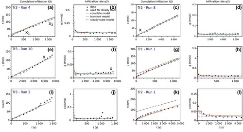
In the previous cases, the non-optimum cases corresponded to descriptions of the transient and steady states of water infiltration that were too parsimonious and inaccurate. However, the physics of flow remained suitable. In other cases, the physics of infiltration changed, and BEST methods were questionable. For instance, some of the cumulative infiltrations exhibited an increase in the infiltration flow rate following the first decrease (Fig. 3(e) and (f) and Fig. 3(i) and (j)). It is clear that after the first part, encompassing both the transient and the steady states, the infiltration rate increased again (Fig. 3(f), x), leading to a slightly convex shape (Fig. 3(e), x). In some cases, the trend was even more marked (Fig. 3(i) and (j)). The increase in the infiltration rate after a certain time evokes the typical effects of water repellency. The water repellency precludes any water infiltration at the beginning of the event, before the soil eventually becomes wet, and the water repellency reduces with time (Lichner et al. 2007). Finally, some of the cumulative infiltrations proved too concave. Related infiltration rates never stopped lowering (Fig. 3(l), x), leading to very concave cumulative infiltrations (Fig. 3(k)). In this case, the analytical model for the transient state had significant difficulties to align on the experimental data. These experimental data pointed to an additional physical factor, reducing water infiltration by too much and over too long a period. The effect of soil layering could be one of the sources of the reduction in water infiltration at the end (Alagna et al. 2016). In these soils, the physics of flow are expected to shift from water infiltration into a uniform profile to water infiltration into a layered profile, when the wetting front reached the bottom layer. Such concave shapes may also result from soil sealing at the surface owing to the effects of water drops (Di Prima et al. 2018).

Despite these shortcomings, in most cases, the water retention and hydraulic conductivity curves could be estimated and depicted for the three methods. The sole exception was the case of transect Tr 2; there being no possibility of obtaining sound values for scale parameter h_g for runs 8 and 9 with the BI method (inappropriate description of transient state). The comparison between the BEST methods is investigated below.

Comparison between BS, BI and BSst methods

The methods gave similar results with subtle differences. The BS method provided values for the scale parameter h_g higher than the means (Fig. 4(a)), and values of K_s lower than the means (Fig. 4(d)). In contrast, the BI and BSst methods gave estimates that were slightly lower for h_g (Fig. 4(b) and (c)) and higher for K_s (Fig. 4(e) and (f)). There are two outliers for the BI method (Fig. 4(b), x) that correspond to the two failures of this method for runs 8 and 9 at transect Tr 2. These data were no longer considered for the statistical analyses. Briefly, the BS method provided higher values for parameter h_g and lower values for K_s, predicting more capillary effects and less conductive soils. These results are in accordance with previous studies of BEST methods (e.g. Bagarello et al. 2014). The predisposition of the BS, BI and BSst methods to follow these trends results from their inherent ways of treating the data, which is the subject of supplementary investigations.

Figure 4. (a, b, c) Estimates for water-pressure head-scale parameter, h_g, and (d, e, f) saturated hydraulic conductivity, K_s, for (a, d) BEST-Slope, BS, (b, e) BEST-Intercept, BI, and (c, f) BEST-Steady-state, BSst, versus method-averaged values, (g, h) fit of experimental distributions to normal laws, and (i) correlation between hydraulic parameters K_s and h_g at the field scale (dashed line) and for each transect (coloured continuous lines).

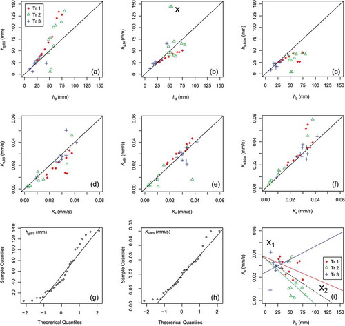
The analysis of the statistical distribution of the parameters clearly demonstrated that parameters h_g and K_s are normally distributed for all BEST methods. The normality of these variables is illustrated by a QQ plot in Figure 4(g) and (h), for the specific case of the BS method. Similar plots can be obtained for the other BEST methods. The QQ plot depicts the theoretical quantiles (admitting a normal law) as a function of experimental quantiles (computed with the experimental data). In the case of normally distributed data, the points align on a straight line. The p values of the Kolmogorov-Smirnov tests are listed in Table 2, and largely exceed the threshold value of 0.05, thus confirming the normality of these variables. Consequently, the arithmetic mean was considered to compute method-averaged parameters, instead of the geometric mean, which applies to log-normal laws. We then computed the arithmetic means from BS, BI and BSst estimates to define the final estimates for h_g and K_s for each BMR run.

Table 2. Normality of distributions (p values) and basic statistics of variables K_s, h_g, IR, and Z_wf, per transect (Tr 1, Tr 2 and Tr 3) and for all data (Total). SD: standard deviation, CV: coefficient of variation.

K-S normality test, p
hg,BS	hg,BI	hg,BSst	hg	Zwf
0.310	0.164	0.774	0.884	0.748
Ks,BS	Ks,BI	Ks,BSst	Ks	IR
0.871	0.571	0.991	0.714	0.852
Basic statistics
	Tr 1	Tr 2	Tr 3	Total
IR (mm/min)
Mean	6.80	3.00	4.66	4.82
SD	1.39	2.64	1.76	2.49
CV	20.4%	87.9%	37.8%	51.7%
Zwf (cm)
Mean	38.0	22.0	26.1	28.7
SD	6.2	12.2	8.7	11.4
CV	16.4%	55.7%	33.4%	39.7%
hg (mm)
Mean	47.6	49.1	23.0	39.9
SD	17.5	24.9	10.1	21.6
CV	36.7%	50.7%	43.9%	54.2%
Ks (mm/s)
Mean	2.84 × 10^−2	1.53 × 10^−2	2.93 × 10^−2	2.43 × 10^−2
SD	7.34 × 10^−3	1.61 × 10^−2	8.35 × 10^−3	1.27 × 10^−2
CV	2.58 × 10^−1	1.06 × 10	2.85 × 10^−1	5.22 × 10^−1

All of the methods allowed the distinction between sorptive and conductive soils. The plot of K_s against h_g defines a straight line with a negative slope (Fig. 4(i)). The upper part of the straight line corresponds to more conductive soils, with less capillarity and more gravity-driven flow (Fig. 4(i), x₁), and the lower part of the straight line corresponds to more sorptive soils, with less gravity and more capillarity-driven flows (Fig. 4(i), x₂). The plot of the same data with respect to the location of the BMR transect shows significant discrepancies. Distinct lines in K_s–h_g may be defined for the three transects, which may indicate the spatial variability at the field scale of soil hydraulic properties (Fig. 4(i), Tr 3 versus Tr 2 versus Tr 1). The intimate relationship between K_s and h_g tends to indicate a significant spatial variability, which is discussed below.

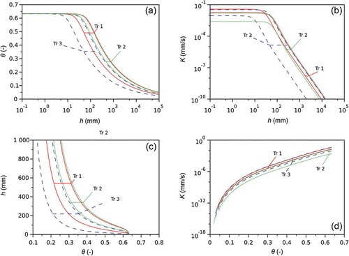
The corresponding water retention and hydraulic conductivity curves are plotted in Figure 5 with respect to the location of the BMR test (transects Tr 1, 2 or 3). To ease the presentation, the water-retention functions are presented for the water-pressure head, h (mm), on both linear (Fig. 5(c)) and log scales (Fig. 5(a)). The hydraulic conductivity is depicted as a function of the water-pressure head with log scales for both axes (Fig. 5(b)), and as a function of the water content (Fig. 5(d)). Note that Figure 5(c) and (d) corresponds to the presentation of the water retention and hydraulic conductivity functions proposed by Lassabatere et al. (2006), whereas more recent presentations use the same format as in Figure 5(a) and (b) (e.g. Lassabatere et al. 2014). On the basis of Figure 5, it is difficult to distinguish any clear trend between transects. The beams of the curves overlap between transects. We note that the curves related to transect Tr 3, and to a lesser extent Transect Tr 1, are positioned more to the left, indicating lower capillarity effects (Fig. 5(a) and (c)). Meanwhile, for transects Tr 3 and Tr 1, the hydraulic conductivity function appears to be higher (Fig. 5(b) and (d)). Briefly, transects Tr 3 and Tr 1 correspond to more conductive soils with less capillarity, whereas transect Tr 2 is less conductive and more prone to water retention by capillarity. However, it remains to be determined whether the three transects define three distinct groups, given the large spreads of values around the mean and the large spread of the hydraulic functions. In the next section we aim to determine whether we can identify the spatial variability at the field scale, or whether the three transects define three comparable groups, and that there is no additional source of spatial variability at the field scale.

Figure 5. (a) water retention curve, Θ(h), (c) water pressure head, h, as a function of water content, Θ, (b) hydraulic conductivity, K, as a function of water pressure head, h, (d) hydraulic conductivity, K, as a function of water content, Θ. Two outlier curves (rings 6 and 9) were removed for Tr 1 to better highlight the main trends.

Studying the spatial variability at the transect and the field scale

We compared statistically the spatial variability at the transect scale (variability between runs obtained at the transect scale) with the variability at the field scale (variability between the three transects). We considered as indicative of the soil hydraulic response the values of IR and Z_wf, and as indicative of the soil hydraulic parameters K_s and h_g (the other hydraulic parameters remained constant for all of the BMR runs), and analysed the decomposition of their variance between the contribution of the explicative variable “transect” and the residual variance (ANOVA tests).

First, we analysed the infiltration rates, IR, and the depths of the wetting front, Z_wf. The two variables are indicative of the bulk soil capacity to infiltrate water, and are plotted in Figure 6(a) and (b). Clearly, IR and Z_wf exhibit a large variability at the transect scale, with a very strong spread around the median for transect Tr 2 (Fig. 6(a) and (b)) and large values for standard deviation and coefficient of variation (Table 2). Given this large dispersion, values of IR and Z_wf overlap between transects, so it is complex to reach any conclusion on the difference between transects. This spread is also strengthened by the outliers with specific behaviours, such as runs 8 and 10 for transect Tr 1, or run 9 for transect Tr 3, with very high infiltration rates, or run 10 for transect Tr 3 with a very low infiltration rate owing to water repellency (Fig. 6(a)).

Figure 6. (a) Spatial variability of averaged infiltration rate IR; (b) depth of the wetting fronts at 10 min, Z_wf; (c) scale parameter for water-pressure head, h_g; and (d) saturated hydraulic conductivity, K_s; transect versus field scales. Open circles correspond to the outliers. For each point, the box plots depict the median value (middle line), the first and the third quartiles, and the first and the last deciles, as well as the outliers, if any (dots with the number referring the position of the ring in the transect).

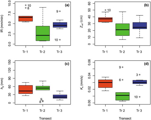
The ANOVA enables us to determine the partition of the total variances into components that are attributable to different sources of variation, i.e. local spatial variation for each transect (transect scale), and between the transects (field scale). ANOVA statistics compare the variance between the transects, and are computed using the differences between medians and the intra-transect variance, which are computed by pooling the variances obtained for the three transects. The results indicate that the inter-transect variance is significant and non-negligible compared with the intra-transect variance for Z_wf (p value of 0.002 for a threshold of significance of 5%, Table 3). Similar results are obtained for IR, with a p value of 0.001 (Table 3), which is even more significant. In other words, the spatial variability at the field scale is as important as the variability at the transect scale. The differences between transects are significant, suggesting a significant spatial variability at the field scale. The sorting of infiltration rates and wetting front depths leads to the following order: Tr 1 > Tr 3 > Tr 2 (Fig. 6(a), Table 2).

Table 3. ANOVA results for the position of the wetting front, Z_wf, infiltration rate, IR, scale parameter for water-pressure head, h_g, and saturated hydraulic conductivity, K_s. The explicative variable is the location of the transect, namely the variable “Transect”. D.f.: degrees of freedom; Sum sq.: sum of squares; Mean sq.: mean squared data; F: Fischer statistic; and p (p value).

	D.f.	Sum sq.	Mean sq.	F	p
IR (mm/min)
Transect	2	72.5	36.2	9.08	0.000964***
Residuals	27	108	3.99
Zwf (cm)
Transect	2	1387	693	7.86	0.00204**
Residuals	27	2380	88.2
hg (mm)
Transect	2	4308	2154	6.29	0.00572**
Residuals	27	9245	342
Ks (mm/min)
Transect	2	0.00124	6.18 × 10^−4	4.32	0.0161*
Residuals	27	0.00345	1.28 × 10^−4

Significance thresholds, ***: <0.0001, **: <0.001, *: <0.01, for p > 0.05.

Similar conclusions can be reached for the variability of the saturated soil hydraulic conductivity, K_s, and the scale parameter for the water-pressure head, h_g. The statistical tests ensure that the variability between transects is significant compared with the variability at the transect scale. Higher values of saturated hydraulic conductivity are found for transects Tr 1 and Tr 3 (Fig. 6(d), Table 2). In contrast, larger values of h_g are found for transect Tr 2 (Fig. 6(c), Table 2). However, from a statistical point of view, the difference between transects is more important for parameter h_g (p = 0.0057, Table 3) than for the saturated hydraulic conductivity (p = 0.016, Table 3). These findings confirm the above statements regarding the water retention and the hydraulic conductivity curves. Transects Tr 1 and Tr 3 appear to be suitable for more conductive soils with less capillarity, the soil being more prone to capillarity at transect Tr 2. These statements can be made despite the significant spreads around the means.

Finally, we investigated the possibility of explaining the values of IR and Z_wf using the two explicative variables, namely the scale parameters h_g and K_s. From a physical perspective, we intended to relate the water infiltration to these two hydraulic parameters, h_g and K_s, and to determine the dependence of this intimate link on the location of the transects. Indeed, these hydraulic parameters and their spatial variability are expected to explain most of the variability observed for water infiltration, and thus variables IR and Z_wf, with the higher scores for the largest values of h_g and K_s. The linear model was run for the complete data set (Table 4 and Fig. 7, black dashed line). We also report the linear models obtained for each transect in Figure 7 (coloured continuous lines).

Table 4. Statistical study of soil hydraulic response (position Z_wf and IR) as a function of soil hydraulic properties (scale parameter for h_g and K_s). The parameters of the linear models, Y = αh_g + βK_s, are listed as follows: Res. std. er.: residual standard error; D.f.: degrees of freedom; Adj. R²: adjusted coefficient of determination; F: Fischer statistic, and p: p value. For the coefficients, their estimates, the standard errors (Std. er.), T statistic and related p value are listed.

	IR (mm/min) ≈ αhg (mm) + βKs (mm/min)
Res. std. er.	D.f.	Adj. R^2	F	p
1.11	27	0.8106	59.59	1.25 × 10^−10***
Coefficient	Estimate	Std. er.	T	p
Intercept	–3.01	0.792	–3.80	0.000747***
hg	0.0741	0.0109	6.78	2.79 × 10^−7***
Ks	200	18.6	10.8	2.78 × 10^−11***
	Zwf (cm) ≈ αhg (mm) + βKs (mm/min)
Res. std. er.	D.f.	Adj. R^2	F	P
5.28	27	0.786	54.1	3.57 × 10^−10***
Coefficient	Estimate	Std. er.	T	p
Intercept	–8.91	3.77	–2.37	0.0254*
hg	0.425	0.0520	8.18	8.77 × 10^−9***
Ks	849	88.4	9.61	3.32 × 10^−10***

Significance thresholds, ***: <0.0001, **: <0.001, *: <0.01, for p > 0.05.

Figure 7. Correlation between depths of wetting fronts Z_wf (b, d) and averaged infiltration rates IR (a, c), and the averaged values of parameters h_g (a, b) and K_s (c, d). Linear models obtained at the field scale (dashed lines) and for each transect (coloured continuous lines).

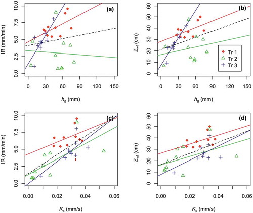
The correspondence is quite conclusive (Fig. 7 and Table 4). Linear models were computed to explain IR and Z_wf as a function of the two hydraulic variables K_s and h_g, the linear models being expressed as IR ≈ αh_g + βK_s and Z_wf ≈ αh_g + βK_s. The statistics indicate significant non-zero values for the coefficients of the contributions of K_s and h_g to the global linear model (Table 4). This indicates that the hydraulic parameters clearly explain the observed hydraulic responses (IR and Z_wf) at the field scale. The plots between predicted variables (IR and Z_wf) and explicative variables (h_g and K_s) show that both hydraulic parameters contribute to the increases in IR and Z_wf (Fig. 7). However, when the linear models are plotted with respect to the transects, different coefficients and linear models are obtained. The intimate link between IR or Z_wf and K_s remains the same, with a similar intercept and slope (Fig. 7(c) and (d), coloured continuous lines versus dashed lines). However, drastic changes are obtained when h_g is considered as the explicative variable (Fig. 7(a) and (b)). These results indicate that there may be a common intimate link between the hydraulic response of the soil and its saturated hydraulic conductivity at the field scale. However, the link between the soil hydraulic response and parameter h_g varies between transects at the field scale.

Conclusions

This paper proposed a new field procedure called Beerkan multi-runs (BMR), which involves carrying out 10 replicates of the Beerkan method at the same place, with rings installed along a 1-m-long transect. Cumulative infiltrations can then be determined and inverted with BEST methods to derive the hydraulic parameters. The depths of the wetting fronts can be determined from cumulative infiltration and water-content measurements.

Such a protocol has many advantages. The large number of replicates permits the more accurate determination of the averaged infiltrations and hydraulic parameters, and spread around the means. It may also enable the identification of specific runs, revealing either the effect of preferential flow or, on the contrary, the impedance of flux owing to water repellency. The large number of replicates also allows the statistical study of correlations between water infiltration and the soil hydraulic parameters at the transect scale. The BMR approach can also be multiplied in the field and performed at several locations. Comparison of the averages between the locations is strengthened by the significant amount of data obtained per location. The whole dataset is designed particularly for the application of the ANOVA, which assesses the relative importance of the variance related to differences between locations to the total variance. From a more physical perspective, such a statistical approach compares the variability observed at the field scale (between locations) with that observed at the transect scale. This approach is particularly suitable for characterizing the spatial variability of water infiltration and soil hydraulic properties and their intimate links. If the physics of water infiltration is properly determined, the link between the hydraulic response and the hydraulic parameters should not deviate drastically from place to place, and the sole spatial variation of hydraulic parameters should explain the spatial variability of water infiltration at both punctual and field scales.

The proposed method showed its efficiency with respect to characterizing the spatial variability of water infiltration, and its link to soil hydraulic properties at several spatial scales. The method is based on the Beerkan method, and is thus easy to apply and not too intensive. In the case of difficult monitoring of several runs simultaneously, the automatic device proposed by Di Prima (2015) could constitute an interesting alternative. Another concern involves the need for separate and independent measures, meaning that any infiltration bulb should not disturb the neighbouring infiltration experiments. In our case, the distance between rings proved sufficient, but this may not be the case for more sorptive and finer soils. This topic requires further investigations, including with respect to modelling aspects and specific methods for deriving hydraulic parameter distributions in the case of interdependent infiltrations.

Acknowledgements

This work was performed within the INFILTRON project supported by the French National Research Agency (ANR-17-CE04-010). The authors would like to thank Artemi Cerdà for his scientific and technical support and for pioneering the idea of Beerkan Multi Runs. The authors would like to thank the associate editor, the editor, and the reviewers for their excellent suggestions and contributions.

Disclosure statement

No potential conflict of interest was reported by the authors.

References

- Alagna, V., et al., 2016. Testing infiltration run effects on the estimated water transmission properties of a sandy-loam soil. Geoderma, 267, 24–33. doi:10.1016/j.geoderma.2015.12.029
- Angulo-Jaramillo, R., et al., 2016. Infiltration measurements for soil hydraulic characterization. Switzerland: Springer Intertnational Publishing. 386 pages.
- Bagarello, V., Di Prima, S., and Iovino, M., 2014. Comparing alternative algorithms to analyze the Beerkan infiltration experiment. Soil Science Society of America Journal, 78 (3), 724. doi:10.2136/sssaj2013.06.0231
- Bagarello, V. and Iovino, M., 2012. Testing the BEST procedure to estimate the soil water retention curve. Geoderma, 187–188, 67–76. doi:10.1016/j.geoderma.2012.04.006
- Bouwer, H., 2002. Artificial recharge of groundwater: hydrogeology and engineering. Hydrogeology Journal, 10 (1), 121–142. doi:10.1007/s10040-001-0182-4
- Braud, I., et al., 2005. Use of scaled forms of the infiltration equation for the estimation of unsaturated soil hydraulic properties (the Beerkan method). European Journal of Soil Science, 56 (3), 361–374. doi:10.1111/ejs.2005.56.issue-3
- Brooks, R. and Corey, A., 1964. Hydraulic properties of porous media. Hydrology Papers, Colorado State University, March.
- Campbell, S.L., Chancelier, J.P., and Nikoukhah, R., 2010. Modeling and Simulation in SCILAB. Modeling and Simulation in Scilab/Scicos with ScicosLab, 4.4. 332 p.
- Cannavo, P., et al., 2010. Spatial distribution of sediments and transfer properties in soils in a stormwater infiltration basin. Journal of Soils and Sediments, 10 (8), 1499–1509. doi:10.1007/s11368-010-0258-7
- Core Team, R., 2013. R: A language and environment for statistical computing. Vienna, Austria: R Foundation for Statistical Computing. Available from: https://www.R-project.org
- Di Prima, S., 2015. Automated single ring infiltrometer with a low-cost microcontroller circuit. Computers and Electronics in Agriculture, 118, 390–395. doi:10.1016/j.compag.2015.09.022
- Di Prima, S., et al., 2016. Testing a new automated single ring infiltrometer for Beerkan infiltration experiments. Geoderma, 262, 20–34. doi:10.1016/j.geoderma.2015.08.006
- Di Prima, S., et al., 2017. Comparing Beerkan infiltration tests with rainfall simulation experiments for hydraulic characterization of a sandy-loam soil. Hydrological Processes, 31 (20), 3520–3532. doi:10.1002/hyp.11273
- Di Prima, S., et al., 2018. Laboratory testing of Beerkan infiltration experiments for assessing the role of soil sealing on water infiltration. CATENA, 167, 373–384. doi:10.1016/j.catena.2018.05.013
- Goutaland, D., et al., 2013. Sedimentary and hydraulic characterization of a heterogeneous glaciofluvial deposit: application to the modeling of unsaturated flow. Engineering Geology, 166, 127–139. doi:10.1016/j.enggeo.2013.09.006
- Hatt, B.E., Fletcher, T.D., and Deletic, A., 2009. Hydrologic and pollutant removal performance of stormwater biofiltration systems at the field scale. Journal of Hydrology, 365 (3), 310–321. doi:10.1016/j.jhydrol.2008.12.001
- Haverkamp, R., et al., 1994. 3-Dimensional analysis of infiltration from the disc infiltrometer .2. Physically-based infiltration equation. Water Resources Research, 30 (11), 2931–2935. doi:10.1029/94WR01788
- Haverkamp, R., et al., 2006. Soil properties and moisture movement in the unsaturated zone. In: J.W. Delleur, ed. The handbook of groundwater engineering. Indiana: CRC Press, 1–59.
- Lassabatere, L., et al., 2006. Beerkan estimation of soil transfer parameters through infiltration experiments-BEST. Soil Science Society of America Journal, 70 (2), 521–532. doi:10.2136/sssaj2005.0026
- Lassabatere, L., et al., 2009. Numerical evaluation of a set of analytical infiltration equations. Water Resources Research, 45, W12415. doi:10.1029/2009WR007941
- Lassabatere, L., et al., 2010. Effect of the settlement of sediments on water infiltration in two urban infiltration basins. Geoderma, 156 (3–4), 316–325. doi:10.1016/j.geoderma.2010.02.031
- Lassabatere, L., 2013. Best method: characterization of soil unsaturated hydraulic properties. In: Caicedo et al. eds. Advances in Unsaturated Soils. London: CRC Press, 527–532.
- Lassabatere, L., et al., 2014. New analytical model for cumulative infiltration into dual-permeability soils. Vadose Zone Journal, 13 (12), 1–15. doi:10.2136/vzj2013.10.0181
- Lichner, L., et al., 2007. Field measurement of soil water repellency and its impact on water flow under different vegetation. Biologia, 62 (5). doi:10.2478/s11756-007-0106-4
- Siltecho, S., et al., 2015. Use of field and laboratory methods for estimating unsaturated hydraulic properties under different land uses. Hydrology and Earth System Sciences, 19 (3), 1193–1207. doi:10.5194/hess-19-1193-2015
- van Genuchten, M.T., 1980. A closed-form equation for predicting the hydraulic conductivity of unsaturated soils. Soil Science Society Of America Journal, 44 (5), 892–898. doi:10.2136/sssaj1980.03615995004400050002x
- Yilmaz, D., et al., 2010. Hydrodynamic characterization of basic oxygen furnace slag through an adapted BEST method. Vadose Zone Journal, 9 (1), 107–116. doi:10.2136/vzj2009.0039
- Yilmaz, D., et al., 2016. Storm water retention and actual evapotranspiration performances of experimental green roofs in french oceanic climate. European Journal of Environmental and Civil Engineering, 20 (3), 344–362. doi:10.1080/19648189.2015.1036128