Pooled flood frequency analysis: a comparison based on peaks-over-threshold and annual maximum series

ABSTRACT

Despite some theoretical advantages of peaks-over-threshold (POT) series over annual maximum (AMAX) series, some practical aspects of flood frequency analysis using AMAX or POT series are still subject to debate. Only minor attention has been given to the POT method in the context of pooled frequency analysis. The objective of this research is to develop a framework to promote the implementation of pooled frequency modelling based on POT series. The framework benefits from a semi-automated threshold selection method. This study introduces a formalized and effective approach to construct homogeneous pooling groups. The proposed framework also offers means to compare the performance of pooled flood estimation based on AMAX or POT series. An application of the framework is presented for a large collection of Canadian catchments. The proposed POT pooling technique generally improved flood quantile estimation in comparison to the AMAX pooling scheme, and achieved smaller uncertainty associated with the quantile estimates.

KEYWORDS:

• peaks-over-threshold
• annual maximum flood
• pooled flood frequency analysis
• homogeneous pooling groups
• site-focused pooling group
• flood seasonality
• L-moments

Editor A. Castellarin Associate editor T. Kjeldsen

1 Introduction

Flood risk assessment based on flood magnitude associated with recurrence interval T (the so-called T-year flood) is important in designing infrastructure, construction and operating river engineering works. Two approaches are commonly considered for modelling of extreme flood events: (1) the annual maximum (AMAX) series and (2) the partial duration series also denoted as peaks-over-threshold (POT). The AMAX series, which uses only the largest flow in each year, may exclude significantly large floods if several of them occurred in a year; and this could result in a loss of flood-related information (Langbein 1949, Lang et al. 1999, Bačová-Mitková and Onderka 2010, Bezak et al. 2014). Another shortcoming of AMAX series is inclusion of some very low discharges in the series that are still the maximum value in the year (Bezak et al. 2014). Thus, incorporation of these events can alter the outcome of the extreme value analysis (Bhunya et al. 2012). However, AMAX series are straightforward to obtain and the most commonly available form of data (FEH 1999). POT data are an alternative to AMAX. The POT model avoids AMAX drawbacks by considering flood peaks above a certain threshold level and allows capturing more information regarding the flood phenomena in comparison with AMAX (Lang et al. 1999). Peaks that are not included in the AMAX series, but are still relatively high, will be considered in the POT series. However, an additional analytical complexity is inherent in the use of POT series. Bezak et al. (2014) described choosing an appropriate threshold level and assuring the independence of the data series as major difficulties in using the POT method. Lang et al. (1999) identified these difficulties as a reason why the POT model remains relatively unpopular and underemployed in the practice of design flood estimation. Solari and Losada (2012) noted the lack of standardized methodology for threshold selection and the difficulty in automating the process as further complications of employing the POT model.

Based on the discussion above, two essential aspects of POT analysis are: (1) determination of the threshold level; and (2) identification of independent exceedences that do not include multiple exceedences associated with the same event (Madsen et al. 1997a). Several methods have been suggested to deal with these two elements. Different criteria have been proposed in the literature to verify the independence hypothesis (e.g. USWRC 1976, Cunnane 1979, FEH 1999). The most commonly accepted practice is to decluster the data (Solari and Losada 2012). Declustering corresponds to filtering the dependent observations (Coles 2001). The exceedences above a threshold that are separated by less than a minimum time span form a cluster. Selecting the maximum value in each cluster helps in achieving the needed statistical independence among the POT observations. Additionally, several approaches have been recommended for appropriate threshold selection. Lang et al. (1999) provided a summary of these approaches. Among proposed threshold selection methods are: fixing the average number of exceedences per year for a specific climate condition or geographical location (Taesombut and Yevjevich 1978, Konecny and Nachtnebel 1985, FEH 1999, Bačová-Mitková and Onderka 2010, Bezak et al. 2014); selection based on a given return period (Dalrymple 1960, Cunnane 1973, Waylen and Woo 1982, Irvine and Waylen 1986); or selection based on a predefined frequency factor $k$: $u=\bar{x}+k{S}_x$ where $\bar{x}$ and $S_x$ are the mean and standard deviation for the series of daily values (Rosbjerg et al. 1992, Madsen and Rosbjerg 1997, Gottschalk and Krasovskaia 2002). Other proposed threshold selection methods are based on a fixed quantile of non-exceedence probability (Solari and Losada 2012), on a verification of the Poisson process hypothesis and dispersion index (Cunnane 1979, Ashkar and Rousselle 1987), or on a graphical method and visual inspection of various plots (Lang et al. 1999, Coles 2001, Burn et al. 2016). The widely used plots include mean residual life plot, which is a plot of the mean flood excess above a given threshold versus a range of threshold values, and a stability plot of the shape parameter of the generalized Pareto exceedences distribution for thresholds higher than a well-chosen level (Burn et al. 2016, Durocher et al. 2018). Durocher et al. (2018) developed a hybrid threshold selection method, where they investigated the behaviour of automatic threshold selection based on the Anderson-Darling goodness of fit test, and then calibrated the automatic method with super regions defined using catchment characteristics. They identified super regions by clustering sites based on drainage area and mean annual precipitation. This classification allows better understanding of the impact of catchment scale and climate for the target site.

Previous research provided insight into the application of AMAX and POT methods in frequency analysis (e.g. Cunnane 1973, Tavares and Da Silva 1983, Madsen et al. 1997b, 1997a, Bačová-Mitková and Onderka 2010, Bhunya et al. 2012). Despite the theoretical basis of the POT model that has helped in its adoption, some practical aspects of flood frequency analysis using AMAX or POT series are still subject to an ongoing debate. Lang et al. (1999) have recommended performing flood frequency analysis with both AMAX and POT models. In either case, the objective is to estimate as accurately as possible the relationship between extreme flood flows and their associated recurrence intervals. Observed flow records used to assess flood frequency at a site are generally short relative to the return period of interest, and spatial coverage of streamgauging stations is sparse, thus limiting the reliability of the needed flood estimates at the site. To overcome this problem and avoid unreliable extrapolation, regional (pooled) information can be used by introducing more data from sites with similar hydrological behaviour to trade between space and time (Zrinji and Burn 1994). Pooled frequency analyses using AMAX series, including the widely used index-flood method, have been applied extensively (e.g. Hosking and Wallis 1993, FEH 1999, Grover et al. 2002, Noto and La Loggia 2009, Saf 2009, O’Brien and Burn 2014). In the context of pooled frequency analysis, only minor attention has been given to the POT method. In fact, only a few studies have performed pooled analysis of POT series, mostly based on an index-flood algorithm, such as the study by Madsen and Rosbjerg (1997). Using simulation, these authors showed their index-flood model to be a robust and efficient estimation method. For small to moderate sample sizes, their regional estimator was superior to the at-site estimator even in extremely heterogeneous regions. Madsen et al. (1997a) compared AMAX and POT series in a regional index-flood context. The performance was evaluated by simulation studies in terms of the accuracy of T-year event estimators. It was demonstrated that for estimation in homogeneous regions, the POT index-flood model in general was more efficient in regions where the distribution function has a negative shape parameter of generalized Pareto distribution, i.e. a distribution with a thick tail that extends to +∞, whereas in regions with positive shape parameter the AMAX model was preferable. In addition to the simulation study, Madsen et al. (1997a) discussed the challenges of identifying homogeneous groups in a real data application; however, they did not provide a comprehensive comparison of the performance of regional estimation methods based on AMAX and POT datasets. Gottschalk and Krasovskaia (2002) provided relations between flood estimates based on AMAX and POT series. Their suggested approach was illustrated using a regional dataset of daily precipitation and runoff records for Costa Rica. Datasets were traditionally subdivided into two different climate and physiographic regions.

To date, POT data have not been widely used in practice despite it having been shown that there are theoretical advantages in using POTs (Madsen and Rosbjerg 1997, Madsen et al. 1997a, Lang et al. 1999). The present research is an effort toward a wider use of the POT method by proposing a standardized methodology and a semi-automated process that can facilitate performing pooled POT frequency analysis by practitioners, especially for large-scale datasets. The objective of the study is to introduce a formalized framework for conducting pooled frequency analysis using data from both POT and AMAX series. This framework employs a recently introduced, practical, and semi-automated method for extracting POT series from hydrometric data. This research takes advantage of a regional POT model introduced by Madsen et al. (1997a), but differs from previous studies that either assumed regional homogeneity or used a subjective grouping of datasets or applied the same basin characteristics partitioning point to define pooling groups of both POT and AMAX datasets. This research differs from these previous studies in that it introduces a systematic approach to construct homogeneous pooling groups and improve quantile estimation which can be adopted in future studies. This framework is verified by comparing the performance of the best identified pooled flood estimation procedure based on POT series with that obtained from a pooled analysis based on AMAX series.

The rest of this paper is organized as follows. Section 2 discusses the methodology involved in the semi-automated POT extraction and provides a general description of the adopted pooled frequency methods. Also introduced in Section 2 are procedures to evaluate the performance of pooled frequency estimation using POT or AMAX series. Section 3 presents an application of the proposed methods, starting with a description of the available data and the extracted POTs for a large collection of hydrometric stations in Canada. This is followed by results and discussion of forming POT- and AMAX-based pooling groups along with comparisons of the pooling techniques. Finally, Section 4 presents conclusions from this study.

2 Methodology

The proposed framework includes a semi-automated process to extract POTs and a formalized method to perform pooled frequency analysis. Required steps to implement the pooling technique involve data screening, super region formation, defining between-site similarities, identifying homogeneous pooling groups, flood quantile estimation and examining the accuracy of quantile estimates. Within the proposed framework, in a first step, AMAX or POT data can be used in the definition of between-site similarities and then, as a second step, either AMAX or POT data can be used to estimate quantiles at a site of interest. Results for each of the four combinations (two methods for defining between-site similarities combined with two methods for quantile estimation) are evaluated to determine a preferred approach. Details of the proposed framework are outlined in the following subsections.

2.1 Peaks-over-threshold extraction

The first step in this analysis is the identification of an appropriate threshold value for recorded flow series, followed by the extraction of POT series based on that selected threshold. The threshold can be selected using the hybrid method developed by Durocher et al. (2018). Their proposed approach facilitates the identification of an effective threshold selection for a dataset containing a large number of sites and it is briefly described in the following.

To satisfy the independence assumption of the extracted peaks, the declustering method presented in Lang et al. (1999) was adopted. The POT extraction method assumes that exceedences above a well-chosen threshold will follow a generalized Pareto distribution, with constant shape parameter. This property is known as threshold stability. In an initial step, the p-value of the Anderson-Darling (AD) goodness of fit test is evaluated for a large range of candidate threshold values and the first threshold associated with a p-value greater than a critical p-value (typically p = 0.25) is considered as the first candidate. This candidate tends to ensure that the generalized Pareto distribution is a reasonable choice. In general, such a threshold will lead to higher accuracy in the estimation of the flood quantile in comparison to other automatic methods. However, in some situations this threshold was found to be too low and thus it does not properly reach threshold stability. A second candidate is obtained by selecting the threshold associated with a fixed exceedence rate. Specific exceedence rates were obtained by comparing the threshold selected according to expert knowledge from 281 hydrometric stations in Canada. A drawback associated with this second candidate is that it can lead to situations where a generalized Pareto distribution is not an appropriate choice. Additionally, the second candidate is generally higher than the first and often results in less accurate estimation of the flood quantiles. The hybrid selection method is a procedure designed to select one of these two candidates. More precisely, if the flood quantile estimate of the first candidate is consistent with the estimate from a threshold associated with a fixed exceedence rate of one event per year, for instance a relative difference between them of less than 15%, then the first candidate is selected, otherwise the higher threshold between the two candidates is selected. This hybrid selection method is shown to remain accurate in the estimation of the flood quantile while mitigating the risk of selecting too low a threshold. The interested reader can refer to Durocher et al. (2018) for further details where specific calibration settings were validated.

2.2 POT pooled flood frequency

2.2.1 Data screening and identifying super regions

The data used in pooled frequency analysis must initially be screened to ensure the satisfaction of the independent and identically distributed (IID) data assumption. The presence of a temporal trend in peak flows will result in rejection of this assumption. Thus, the extracted POTs are evaluated in terms of trends in the individual exceedences using the Mann-Kendall nonparametric trend test (Mann 1945, Kendall 1975). The presence of statistically significant serial correlation in data series can impair the robustness of trend detection (Wang et al. 2015). To mitigate the impact of serial correlation, the block bootstrap (BBS) approach (Önöz and Bayazit 2012) is employed in conjunction with the trend test. Trends in the number of events over time (counts) for individual POT series are evaluated using logistic regression (please refer to Frei and Schär (2001) for more details on logistic regression). The screened data can then be utilized to construct pooling groups.

The proposed methodology examines the effect of major classification of sites based on their catchment physiographic and climatologic attributes as an initial step in pooled flood frequency. Mean annual precipitation (MAP) and basin area were selected as catchment descriptor surrogates of climate and scale controls. Studies have shown that these catchment descriptors exert significant control on the frequency regime of hydrological extremes (see Salinas et al. (2014) and references therein). Clusters of sites, known here as super regions, are formed by grouping sites based on similarity in drainage area and MAP.

2.2.2 Pooling group formation

In pooled flood frequency analysis, extreme event information from a collection of sites that show similar extreme hydrological behaviour is pooled to help improve the accuracy of the extreme flow estimation at a target site. The goal is to form pooling groups that approximately satisfy the homogeneity condition. In each pooling group, the sites’ frequency distributions are identical apart from a site-specific scale factor (Hosking and Wallis 1997). Identification of these pooling groups is an important component of pooled flood frequency analysis (Burn et al. 1997). Different approaches exist to delineate these pooling groups. In this study, the focused pooling group approach (Reed et al. 1999) was employed. The focused pooling group approach selects a potentially unique group of catchments that are most comparable to the target site to form a pooling group for that site. The focused pooling group approach and its modifications have been applied extensively as a pooling technique in flood frequency analysis (e.g. Zrinji and Burn 1994, 1996, Tasker et al. 1996, Burn 1997, FEH 1999, Castellarin et al. 2001, Grover et al. 2002, Latraverse et al. 2002, Eng et al. 2005, Merz and Blöschl 2005, Shu and Ouarda 2008, Das and Cunnane 2011, Micevski et al. 2015). This approach typically involves defining similarity between sites and a cut-off point that determines whether or not to include a site in the pooling group.

Identification of pooling groups of similar sites is the next critical step in performing pooled flood frequency analysis. Selection of variables to define similarity (or dissimilarity) between catchments is an essential prerequisite in this stage (Burn 1997). In this study, hydrological response properties concerning the timing and variability of peak flow events are explored. Catchments showing similarity in these variables can be considered as potential members of the same pooling group for pooled flood frequency analysis (Ouarda et al. 2006). These variables will henceforth be called seasonality measures.

2.2.3 Flood seasonality measures

Since their introduction into the hydrological literature, seasonality measures have been successfully employed as a measure of similarity in catchment hydrological response in several studies (Bayliss and Jones 1993, Burn 1997, Cunderlik et al. 2004, O’Brien and Burn 2014).

The angular value of the date of a peak occurrence is calculated following Burn (1997) by:

(1) ${\theta }_i={\left(\mathrm{J}\mathrm{u}\mathrm{l}\mathrm{i}\mathrm{a}\mathrm{n}\mathrm{D}\mathrm{a}\mathrm{t}\mathrm{e}\right)}_i\frac{2\pi }{\mathrm{l}\mathrm{e}\mathrm{n}\mathrm{y}\mathrm{r}}$(1)

where θ_i is the angular value (radians) for the date of occurrence for event i, and lenyr is the number of days in a year. For a sample of n events, the coordinates of the mean flood date are defined as:

(2a) $\bar{x}=\frac{1}{n}{\sum }_{i=1}^n\mathrm{c}\mathrm{o}\mathrm{s}({\theta }_i)$(2a)

(2b) $\bar{y}=\frac{1}{n}{\sum }_{i=1}^n\mathrm{s}\mathrm{i}\mathrm{n}({\theta }_i)$(2b)

where n is the number of peak events and $\bar{x}$ and $\bar{y}$ are the coordinates of mean flood date. The mean event date can be determined by:

(3) $\mathrm{M}\mathrm{D}=\mathrm{t}\mathrm{a}{\mathrm{n}}^{-1}\left(\frac{\bar{y}}{\bar{x}}\right)\left(\frac{\mathrm{l}\mathrm{e}\mathrm{n}\mathrm{y}\mathrm{r}}{2\pi }\right)$(3)

where MD is a measure of the average time of occurrence of the flood event for a given catchment. A measure of the variability of the occurrences of peak events can be defined through:

(4) $\bar{r}=\sqrt{{\bar{x}}^2+{\bar{y}}^2}$(4)

where $\bar{r}$ ranges from 0 (low regularity) to 1 (high regularity) and represents the dimensionless spread of the data for each catchment.

Chen et al. (2013) pointed out the importance of including flood magnitude information in the definition of flood seasonality and suggested using it as a weight to consider the effect of event magnitude in defining the timing and regularity of flood events as follows:

(5a) ${\bar{x}}^{\prime }=\frac{\sum _{i=1}^n{q}_i\mathrm{c}\mathrm{o}\mathrm{s}({\theta }_i)}{\sum _{i=1}^n{q}_i}$(5a)

(5b) ${\bar{y}}^{\prime }=\frac{\sum _{i=1}^n{q}_i\mathrm{s}\mathrm{i}\mathrm{n}({\theta }_i)}{\sum _{i=1}^n{q}_i}$(5b)

where q_i is the flow magnitude for event i.

In the next step of the analysis, the seasonality measures discussed above are employed in the definition of the similarity/dissimilarity between catchments.

2.2.4 Similarity statistics

A single numeric that defines the separation (distance) of two catchments in the seasonality space is used to define dissimilarity. Several distance metrics have been suggested in the past (e.g. Lance and Williams 1966, Webster and Burrough 1972, Castellarin et al. 2001). The separation of two catchments in seasonality space based on Euclidean distance is defined as:

(6) $D_{ij}={\left[{\sum }_{m=1}^M{\left(x_m^i-x_m^j\right)}^2\right]}^{1/2}$(6)

where D_ij is the distance (dissimilarity) between catchments i and j; $x_m^i$ is the value of the mth hydrological response property for catchment i; and M is the number of considered characteristics. A smaller value of D_ij demonstrates more similarity between two corresponding catchments in flood seasonality space.

2.2.5 Catchment grouping process

Different strategies are available to finalize the pooling group for each site. Castellarin et al. (2001) stated that the homogeneity of a pooling group and its size are two fundamental principles in effective identification of pooling groups. Burn and Goel (2000) implied that pooling groups should be sufficiently large. In the Flood Estimation Handbook (FEH 1999) it is suggested that a pooling group should ideally contain 5T station-years of data to provide an effective quantile estimate at return period T. Hosking and Wallis (1997) stated that no substantial benefit is gained when forming regions with more than 20–25 sites. In this study, the first 25 sites with minimum pairwise dissimilarities with the target site were selected as initial pooling groups while ensuring that there are at least 500 station-years of data in the pooled group. For each site, four different types of initial pooling groups were created using different combinations of seasonality measures discussed for POT series.

The initial pooling groups obtained from the above technique are evaluated for homogeneity. For this purpose, the commonly used homogeneity test (H statistic) proposed by Hosking and Wallis (1993) was used. Please refer to Hosking and Wallis (1997) for more details on this test. The H statistic was recommended as a guideline to consider a pooling group homogeneous ($H<1$), possibly heterogeneous ($1\le H<2$), and heterogeneous ($H\ge 2$).

If there is heterogeneity in the initial pooling group, revisions are performed on the pooling group while still satisfying the target number of station-years. The approach taken for revision is that catchments whose removal leads to the greatest improvement in the homogeneity statistic of the group are sequentially removed from the pooling group to enhance the group homogeneity while maintaining 500 station-years of data.

2.2.6 Flood quantile estimation

The identified pooling groups can then be used to estimate the pooled flood quantile for POT flow series. This study follows Madsen and Rosbjerg (1997) and Madsen et al. (1997a) for pooled flood modelling of POT series and quantile estimation. The model is composed of the most commonly used Poisson distribution for modelling the number of threshold exceedences in any fixed time interval (Önöz and Bayazit 2001) and the most commonly used generalized Pareto (GP) distribution for modelling the exceedences (e.g. Van Montfort and Witter 1985, Rosbjerg et al. 1992, Lang et al. 1999, Solari et al. 2017, Durocher et al. 2018). Hosking and Wallis (1997) goodness of fit test can also be applied to identify the appropriate 2-parameter distribution for POT series. The model is described below following Madsen and Rosbjerg (1997).

2.2.6.1 At-site T-year flood quantile

By allowing $q_i$ to be the time series of flows for the site of interest, introducing a threshold level $q_0$, and considering the independence criteria, the POT series is obtained using $x_i=q_i-q_0$. The occurrence of peaks is assumed to follow a Poisson process, so the number of exceedences N in t years is Poisson distributed with the following probability function:

(7) $\begin{array}{rl}& P\left\{N\left(t\right)=n\right\}=\frac{{\left(\lambda t\right)}^n}{n!}exp\left(-\lambda t\right)\\ & n=0,1,2,\dots \end{array}$(7)

where $\lambda$ equals the expected number of exceedences per year and can be estimated by:

(8) $\hat{\lambda }=\frac{N}{t}$(8)

The exceedence magnitudes $x_i$ are assumed to be independent and identically distributed following the GP distribution. The cumulative distribution function of GP with the scale and shape parameters $\sigma$ and $\xi$, respectively, is:

(9) $\left\{\begin{array}{c}F\left(x\right)=1-exp\left(-\frac{x}{\sigma }\right)\xi =0\\ F\left(x\right)=1-{\left(1-\xi \frac{x}{\sigma }\right)}^{1/\xi }\xi \ne 0\end{array}\right.$(9)

For $\xi =0$ (in the limit), the GP distribution reduces to the exponential distribution. The range of x is $0\le x<\mathrm{\infty }$ for negative shape parameters, whereas an upper limit, $0\le x<\sigma /\xi$ exists for positive shape parameters.

The T-year event, $x_T$, is defined as the $\left(1-1/\lambda T\right)$ quantile in the distribution of threshold exceedences. Therefore, by inverting Equation (9) one obtains:

(10) $\left\{\begin{array}{c}{x}_T=F^{-1}\left(1-1/\lambda T\right)=\sigma \times ln\left(\lambda T\right)\xi =0\\ x_T=F^{-1}\left(1-1/\lambda T\right)=\frac{\sigma }{\xi }\left[1-{\left(1/\lambda T\right)}^{\xi }\right]\xi \ne 0\end{array}\right.$(10)

The L-moment estimates of the GP distribution parameters are given by:

(11) $\hat{\sigma }={\hat{\lambda }}_1\left(\frac{1}{{\hat{\tau }}_2}-1\right)$(11)

(12) $\hat{\xi }=\frac{1}{{\hat{\tau }}_2}-2$(12)

where ${\hat{\lambda }}_1$ is an estimate of the first L-moment and ${\hat{\tau }}_2$ is an estimate of L coefficient of variation. The reader is referred to Hosking (1990) for further details on the L-moments estimates.

2.2.6.2 Pooled T-year flood quantile

Consider a pooling group to have M sites with POT records $x_{ij}$, where $i=1,2,\dots ,M$ and $j=1,2,\dots ,N_i$. The index-flood method assumes that the distributions of events at different sites in the pooling group are identical (unique growth curve for the pooling group) except for scale (index-flood parameter). Employing the mean of exceedences as the index-flood parameter, Madsen and Rosbjerg (1997) expressed the pooled T-year event estimator as:

(13) ${\hat{x}}_{T_i}={\hat{\mu }}_t\frac{1+{\hat{\xi }}^R}{{\hat{\xi }}^R}\left[1-{\left(\frac{1}{{\hat{\lambda }}_{t}T}\right)}^{{\hat{\xi }}^R}\right]$(13)

That is, the mean estimate of the exceedences, ${\hat{\mu }}_t$, and the Poisson parameter estimate, ${\hat{\lambda }}_t$ are calculated from at-site data, whereas the shape parameter is estimated from the pooled data. To estimate the pooled shape parameter, ${\hat{\xi }}^R$, the weighted average of L-moment ratios is used as follows:

(14) ${\hat{\xi }}^R=\frac{1}{{\hat{\tau }}_2^R}-2$(14)

(15) ${\hat{\tau }}_2^R=\frac{{\sum }_{i=1}^M{w}_i{\hat{\tau }}_2^{\hspace{0.17em}}}{{\sum }_{i=1}^M{w}_i}$(15)

where $w_i$ is equal to the record length, in years, at site i. Madsen and Rosbjerg (1997) indicated that cross-correlation may have a significant impact on the regional shape parameter estimator. Interaction between site cross-correlation and estimation of the regional shape parameter is an area of future research. Employing the quantile estimation methods described above, the pooled and at-site quantiles were determined for all the pooling groups identified.

2.3 AMAX pooled flood frequency

AMAX pooled frequency analysis follows proposed steps similar to those described for the POT dataset in Section 2.2. AMAX series are extracted for the same set of hydrometric stations and seasonality measures are estimated for AMAX series at each station. Initial focused pooling groups are then formed for each station using close stations in the seasonality space within each identified super region. Revisions to the pooling groups are performed as necessary. Following the Hosking and Wallis (1997) methodology for index-flood frequency analysis, the best frequency distribution is identified for each pooling group and pooled quantiles are estimated. In this study, the generalized logistic, generalized extreme value (GEV), generalized normal, Pearson type III, and generalized Pareto models were considered as potential candidates for the frequency distribution.

2.4 Approach to evaluate POT and AMAX pooling groups

A focus of this research is to provide means of investigating the performance of pooling techniques in quantile estimation using both POT and AMAX series. Two sets of analyses are proposed to compare the performance of AMAX- and POT-based pooling groups. As discussed, AMAX and POT data are used in the definition of between-site similarities and, with each of these two possibilities, AMAX and POT data are used to estimate quantiles at a site of interest following the discussed quantile estimation method. The obtained quantiles for each of the following four combinations, as described in Table 1, are evaluated to determine a preferred approach.

Table 1. Combinations of similarity measures and extreme flow data.

		Between-site similarity
		AMAX	POT
Quantile estimation using:	AMAX	AA	PA
	POT	AP	PP

It is expected that employing AMAX versus POT in defining pooling groups will result in diverse pooling groups with unequal performance. Thus, it is essential to evaluate the performance of distinctive pooling groups to select the best performing pooling method. Two methods are presented here to conduct the evaluation, one based on errors in quantile estimates and the other based on the width of confidence limits, as discussed below.

2.4.1 Error in quantile estimates

The FEH (1999) introduced an estimate of uncertainty in the resulting pooled growth curve as one way of evaluating different pooling groups. A similar approach that summarizes the average difference between pooled and at-site growth curves at various return periods has been adopted in this study. This measure is obtained by averaging over the sites with long flow records, since it can be assumed they provide reliable at-site estimates. For all long-record sites, the T-year at-site and pooled growth curves are obtained using the identified pooling groups. The measure of associated error in the pooled growth curve for different return periods is described as follows:

(16) $\mathrm{R}\mathrm{M}\mathrm{S}{\mathrm{E}}_T=\sqrt{\frac{{\sum }_{i=1}^{N_{\mathrm{l}\mathrm{o}\mathrm{n}\mathrm{g}}}{\left(\mathrm{l}\mathrm{n}{q}_{T_i}-\mathrm{l}\mathrm{n}{q}_{T_i}^P\right)}^2}{N_{\mathrm{l}\mathrm{o}\mathrm{n}\mathrm{g}}}}$(16)

where $\mathrm{R}\mathrm{M}\mathrm{S}{\mathrm{E}}_T$ is an uncertainty measure for return period T, $N_{\mathrm{l}\mathrm{o}\mathrm{n}\mathrm{g}}$ is the number of long-record sites, $q_{T_i}$ is the T-year site growth factor for site i, and $q_{T_i}^P$ is the T-year pooled growth factor for site i. Lower values of $\mathrm{R}\mathrm{M}\mathrm{S}{\mathrm{E}}_T$ indicate a superior pooling group.

In addition to $\mathrm{R}\mathrm{M}\mathrm{S}{\mathrm{E}}_T$ for different return periods, $\mathrm{R}\mathrm{M}\mathrm{S}{\mathrm{E}}_F$ is used to compare the entire at-site and pooled frequency distributions. $\mathrm{R}\mathrm{M}\mathrm{S}{\mathrm{E}}_F$ is defined as follows for each long-record site:

(17) $\mathrm{R}\mathrm{M}\mathrm{S}{\mathrm{E}}_{F_i}=\sqrt{\frac{{\sum }_{j=1}^t{\left(\frac{\mathrm{l}\mathrm{n}{q}_{T_j}-\mathrm{l}\mathrm{n}{q}_{T_j}^P}{\mathrm{l}\mathrm{n}{q}_{T_j}}\right)}^2}{t}}$(17)

where $\mathrm{R}\mathrm{M}\mathrm{S}{\mathrm{E}}_{F_i}$ is an uncertainty measure between at-site and pooled quantiles for site i, t is the number of return periods estimated, $q_{T_j}$ is the T_j-year site growth factor, and $q_{T_j}^P$ is the T_j-year pooled growth factor.

2.4.2 Confidence-interval ratio

Uncertainty in the pooled quantile estimates is utilized as the second method of evaluation. In this study, uncertainty quantified by constructing confidence intervals for estimated quantiles is explored. Among approaches to assess uncertainty, the parametric resampling approach (Hosking 2013) is adopted to construct confidence intervals for pooled quantiles. This approach generates realizations of data in the pooling group and requires specification of a frequency distribution for the pooling group. This approach reflects the average cross-correlation between sites in the pooling group and accounts for the existence of heterogeneity within the group. Hosking (2013) reported that this approach provides more realistic estimates of confidence intervals.

The basis of the comparison is the width of the 95% confidence interval. A narrower confidence interval indicates a more precise estimate and is preferred to an estimate with wider confidence interval. In this study, the ratio of the width of the confidence interval to the quantile estimate for each return period is proposed as a measure of performance of the pooling groups.

3 Application

The presented framework to perform pooled frequency analysis for AMAX and POT series in the context of super regions is demonstrated on a collection of hydrometric stations in Canada. Model performance and comparisons are also evaluated.

3.1 Description of dataset and study area

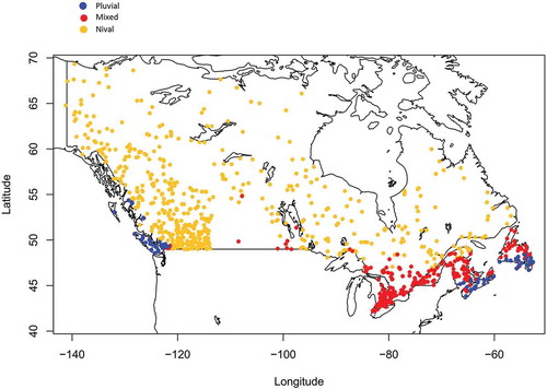
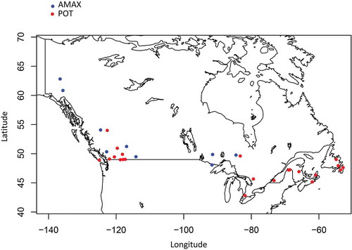
The suggested approach in this research is illustrated using flow records from a collection of hydrometric gauges, with unregulated flows, located across Canada. Trends in AMAX series were initially examined for the available dataset; removing 224 stations with trends in the AMAX data reduced the dataset to 919 stations. Figure 1 shows the locations of these gauges. The large diversity of geographical, meteorological, and hydro-climatic conditions in Canada is an inevitable challenge for such a vast database.

Figure 1. Location of hydrometric stations with different hydrological regimes.

3.1.1 POT flow series

Following Burn and Whitfield (2016), the collection of sites was reviewed to identify the dominant hydrological regime using the mean date of occurrence of flood events in the seasonality space. For more information please refer to Burn and Whitfield (2016). Figure 1 illustrates the locations of the stations with nival, mixed and pluvial regimes in geographical space. Stations displaying pluvial and mixed flood response are mostly located on the east and west coasts of Canada, and some in southern Ontario. Central parts of Canada and higher latitudes mostly correspond to the nival regime. Initially the average number of peaks to be extracted per year (PPY) was bounded between 1 and 5. In light of the nature of catchment flows in Canada and the existence of different hydrological regimes dominated by snowmelt, rainfall or mixed events, assembling up to 5 PPY was considered to provide sufficient extreme event information when using POT series rather than AMAX (PPY = 1). Next, the hybrid threshold selection method was applied to the dataset and, based on the algorithm of the adopted threshold selection method, the best threshold was identified from the set of initial thresholds yielding 1–5 PPY for each station. For gauges with the nival hydrological regime, for which flood events correspond to snowmelt response, the maximum of 5 PPY was considered to be too high a value. For the case of stations having a mostly nival regime, the upper bound of 2.5 PPY was considered for identifying the best threshold. For each station, based on the discussed criteria, a threshold was identified, and POT series were extracted. The maximum likelihood parameter estimation technique within the hybrid threshold selection method was unable to fit a GP distribution to the POT series of 25 stations. Thus, they were removed from the rest of the analysis. Figure 2 provides the frequency of identified PPY for the stations.

Figure 2. Histogram of range of peaks per year (PPY) selected for the hydrometric stations.

The next step of data screening involves trend analysis. For the set of POT series obtained, trends in both exceedence magnitudes and number of events per year over time for individual stations were examined at 5% significance level. Table 2 provides a summary of the trend test analysis. For a larger number of stations, a significant trend in number of events per year was identified rather than trend in exceedence magnitudes. Increasing trend in number of events per year was shown by 14.88% of sites, while only 4.47% had decreasing trend. There were fewer stations (52) with significant trends in exceedence magnitudes, 1.57% of total number of stations exhibiting increasing and 4.25% of stations decreasing trend. For the rest of the analysis, sites having trend in either the magnitude of exceedences or the number of events per year were excluded, with 684 stations remaining in the dataset.

Table 2. Summary of trend analysis of POT data for 894 hydrometric stations.

	Increasing	Decreasing
Trend in exceedence magnitude	14 (1.57%)	38 (4.25%)
Trend in number of events per year	133 (14.88%)	40 (4.47%)

3.1.2 AMAX flow series

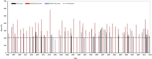
The AMAX series representing the highest flow value in each year was also extracted for the same set of data. Both POT and AMAX contain some of the highest extreme values, while lesser magnitude extreme flows might only appear in the POT series or only in the AMAX series, as can be seen from Figure 3, which provides an example of differences in the amount of data acquired with AMAX and POT series.

Figure 3. Example of data obtained from AMAX and POT series for a hydrometric station.

3.1.3 Super regions

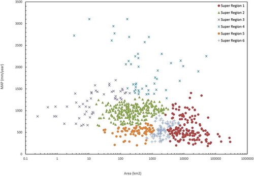
As was proposed in the Methodology section, drainage area and MAP are used to group the catchments into subsets (super regions) that represent similar properties in the size of drainage area and amount of annual precipitation. Following Mostofi Zadeh and Burn (2019), agglomerative hierarchical clustering is used to form super regions. For the dataset of catchments under study, six super regions were identified after preliminary trials as they enhance the representation of variation in drainage area and precipitation. Figure 4 plots MAP against drainage area for the catchments under study; the six super regions are also presented in this figure.

Figure 4. Super regions based on characteristics of hydrometric stations.

3.2 Results and discussion

3.2.1 Analysis of POT-based pooling groups

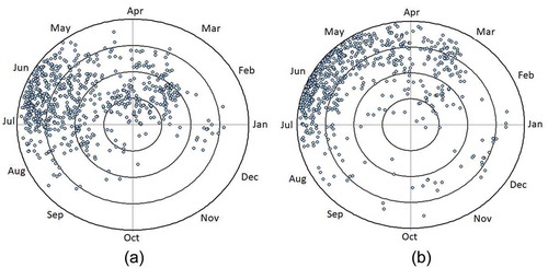
Figure 5(a) plots the catchments in unweighted seasonality space, based on POT events, for the dataset under study. Within each super region, the seasonality statistics, $\bar{x}$ and $\bar{y}$, and also their weighted modifications, were employed in the definition of between-site dissimilarity using Euclidean distance in the seasonality space. Table 3 provides the summary of average homogeneity test results for the identified pooling groups in all the super regions. A considerable number of the pooling groups formed using POT series (PP) were classified as homogeneous (>87.1%) and a small percentage (<12.9%) as possibly homogeneous. Hosking and Wallis (1997) indicate that moderately heterogeneous regions may still offer valuable information concerning quantile estimates for extreme events. Constructing pooling groups with different seasonality measures does not result in a substantive change in homogeneity, as can be seen by comparing the rows in Table 3. Adopting the methodology described in Section 2.2.6, flood quantiles were estimated for different return periods, for both cases of considering only at-site data and using pooling groups.

Table 3. Summary of the homogeneity tests for pooling groups formed by POT statistics.

	$H<1$	$1\le H<2$	$H\ge 2$
	Homogeneous	Possibly homogeneous	Heterogeneous
POT series (PP)
$\bar{x}$ and $\bar{y}$	89.9%	10.1%	0%
Weighted $\bar{x}$ and weighted $\bar{y}$	87.1%	12.9%	0%
AMAX series(PA)
$\bar{x}$ and $\bar{y}$	87.3%	13.6%	1.8%
Weighted $\bar{x}$ and weighted $\bar{y}$	83.3%	12.9%	3.8%

Figure 5. Mean flood date in unweighted seasonality space for (a) POT series and (b) AMAX series.

The approach discussed in Section 2.4 was employed to compare the performance of pooling groups containing POT or AMAX series. The homogeneity of the pooling groups using AMAX data (PA) was also examined; the results are provided in the two bottom lines of Table 3. Similar to the case of POT pooling groups (PP), the approach taken resulted in a large number of homogeneous pooling groups. Next, following the methodology of Hosking and Wallis (1997), the frequency distribution with best fit to each pooling group was identified. This was followed by quantile estimations using both pooled and at-site data.

3.2.2 Analysis of AMAX-based pooling groups

In the same manner as with POT series, this time AMAX statistics were employed to construct pooling groups. Seasonality statistics were estimated using AMAX data. Figure 5(b) plots the catchments in unweighted seasonality space, based on AMAX events. By comparing Figure 5(a) and 5(b) one can conclude that AMAX events are more regular ($\bar{r}$ closer to 1), especially for sites having snowmelt events with mean flood date between mid-spring and mid-summer (nival regime). Lower regularity in the POT series is inevitable since there is more than one extreme flow event per year and these events have different occurrence times.

Table 4 provides a summary of the homogeneity test for pooling groups formed using AMAX data (AA). Again, for a large portion of stations (>85.4%) homogeneous pooling groups, for a small percentage (<11.8%) possibly homogeneous pooling groups, and for a few (<2.8%) heterogeneous pooling groups were identified. No substantive differences are noted when employing the two different seasonality measures, namely the one based on the unweighted statistics of Equation (2) and the other based on the weighted statistics of Equation (5). The best-fit distribution to the pooled data was determined and flood quantiles were estimated for different return periods, for both at-site data and using pooling groups.

Table 4. Summary of the homogeneity tests for pooling groups formed by AMAX statistics.

	$H<1$	$1\le H<2$	$H\ge 2$
	Homogeneous	Possibly homogeneous	Heterogeneous
AMAX series (AA)
$\bar{x}$ and $\bar{y}$	85.4%	11.8%	2.8%
Weighted $\bar{x}$ and weighted $\bar{y}$	87.1%	11.4%	1.5%
POT series (AP)
$\bar{x}$ and $\bar{y}$	85.5%	14.5%	0%
Weighted $\bar{x}$ and weighted $\bar{y}$	86%	14%	0%

The approach discussed in Section 2.4 was employed to facilitate the performance comparison of pooling groups containing AMAX or POT series. In this experiment, additional information (POT events) was introduced in the pooling groups (AP). The pooling groups including new data were also inspected for their homogeneity. The results are provided in the bottom two lines of Table 4 and reveal a high percentage of pooling groups (>85.5%) that can be considered homogeneous. Likewise, at-site and pooled quantile estimates for the new pooling groups containing POT series were estimated.

3.2.3 POT and AMAX pooling group comparison

3.2.3.1 Error in quantile estimates

The $\mathrm{R}\mathrm{M}\mathrm{S}{\mathrm{E}}_T$ described in Equation (16) was studied for four types of pooling groups: those formed by POT seasonality measures (either PP or PA), and those formed by their AMAX counterparts (AA, AP). A total of $\left(N_{\mathrm{l}\mathrm{o}\mathrm{n}\mathrm{g}}=\right)$32 stations, with AMAX series longer than 60 years, were considered for this analysis.

Table 5 (left half) lists the $\mathrm{R}\mathrm{M}\mathrm{S}{\mathrm{E}}_T$ estimates for pooling groups formed by POT seasonality measures using both the POT series (PP) and the AMAX series (PA) in the pooling group. Investigating Table 5 reveals that, regardless of the seasonality measures used to construct the pooling groups, PP groups to estimate the quantiles have lower RMSE compared with the PA pooling groups. The POT series benefited from using larger amounts of pooled information and therefore higher accuracy quantile estimates were obtained. By looking at these results one can conclude that, for PP, pooling groups formed using weighted $\bar{x}$ and $\bar{y}$ seasonality measures resulted in the lowest $\mathrm{R}\mathrm{M}\mathrm{S}{\mathrm{E}}_T$, while for the PA method, pooling groups formed using $\bar{x}$ and $\bar{y}$ seasonality measures resulted in the lowest $\mathrm{R}\mathrm{M}\mathrm{S}{\mathrm{E}}_T$.

Table 5. Summary of $\mathrm{R}\mathrm{M}\mathrm{S}{\mathrm{E}}_T$ of different pooling techniques using POT (AMAX) series. Bold indicates best result in each row.

	PP(PA)				AP(AA)
Return period	$\bar{x}$ and $\bar{y}$		Weighted $\bar{x}$ and $\bar{y}$		$\bar{x}$ and $\bar{y}$		Weighted $\bar{x}$ and $\bar{y}$
2	0.025	(0.050)	0.023	(0.058)	0.025	(0.051)	0.024	(0.048)
5	0.030	(0.038)	0.031	(0.048)	0.029	(0.041)	0.030	(0.037)
10	0.059	(0.078)	0.058	(0.100)	0.058	(0.083)	0.056	(0.072)
20	0.094	(0.122)	0.098	(0.152)	0.092	(0.130)	0.088	(0.113)
50	0.144	(0.182)	0.136	(0.218)	0.140	(0.193)	0.133	(0.171)

The right half of Table 5 depicts the $\mathrm{R}\mathrm{M}\mathrm{S}{\mathrm{E}}_T$ estimates for pooling groups formed by AMAX statistics using both AMAX series (AA) and POT series (AP) in the pooling group. The AP pooling groups are seen here to produce lower $\mathrm{R}\mathrm{M}\mathrm{S}{\mathrm{E}}_T$ than the AA pooling groups. Greater improvements can be seen for longer return periods. It can be inferred from Table 5 that employing the weighted $\bar{x}$ and $\bar{y}$ seasonality measure produced the lowest $\mathrm{R}\mathrm{M}\mathrm{S}{\mathrm{E}}_T$ among AP pooling groups (bold numbers), and also AA pooling groups.

A parallel comparison of the left and right divisions of Table 5 concludes that pooling groups formed with the AMAX seasonality statistics (either AA or AP) are superior to those formed by their POT-based counterparts (either PP or PA). To point out the best performing quantile estimation method, one can select the weighted $\bar{x}$ and $\bar{y}$ seasonality measure of AMAX data to identify similar stations as inputs in pooling groups. Using the AA pooling method and the AP pooling method in this pooling scheme results in the lowest $\mathrm{R}\mathrm{M}\mathrm{S}{\mathrm{E}}_T$ for AMAX and POT flow series, respectively. For the rest of the analysis only these two combinations were examined further.

To better indicate the merits of employing super regions as an initial step in the proposed pooling scheme, another experiment was conducted without using super regions. The dataset was treated as a whole and best pooling groups were identified with similar approaches as discussed before. Table 6 summarizes the parallel comparison of $\mathrm{R}\mathrm{M}\mathrm{S}{\mathrm{E}}_T$ for the best identified AMAX and POT pooling technique, AA and AP, respectively, with and without using super regions. Employing the super region approach was found to improve $\mathrm{R}\mathrm{M}\mathrm{S}{\mathrm{E}}_T$ in both AMAX (AA) and POT (AP) pooling groups formation.

Table 6. Summary of $\mathrm{R}\mathrm{M}\mathrm{S}{\mathrm{E}}_T$ with or without employing super regions. Bold indicates best result in each row.

	With super regions		Without super regions
Return period	AP	AA	AP	AA
2	0.024	0.048	0.056	0.076
5	0.030	0.037	0.064	0.068
10	0.056	0.072	0.086	0.090
20	0.088	0.113	0.112	0.119
50	0.133	0.171	0.145	0.178

In addition to $\mathrm{R}\mathrm{M}\mathrm{S}{\mathrm{E}}_T$ for different return periods, $\mathrm{R}\mathrm{M}\mathrm{S}{\mathrm{E}}_F$ as defined in Equation (17) was also examined to compare the entire at-site and pooled frequency distribution. Table 7 lists the $\mathrm{R}\mathrm{M}\mathrm{S}{\mathrm{E}}_F$ of long-record sites with pooling groups formed based on best performing POT (AP) and AMAX (AA) pooling techniques. Investigating Table 7 reveals that using the AP pooling technique will generally result in lowering the $\mathrm{R}\mathrm{M}\mathrm{S}{\mathrm{E}}_F$, although some stations do not follow this general pattern. Figure 6 shows the location of long-record stations where $\mathrm{R}\mathrm{M}\mathrm{S}{\mathrm{E}}_F$ of AMAX (AA) or POT (AP) pooling groups are superior. The AP pooling technique surpasses the AA approach for the majority (69%) of long-record stations. These stations are located mostly in coastal areas and the southeastern part of the country. Table 8 summarizes the information about the stations where AA quantile estimation was superior. Instances where the AA pooling approach improved the quantile estimation were associated with hydrometric stations belonging to regions identified with the nival regime and mostly snowmelt events. This implies that stations with the nival regime and smaller PPY may benefit less from the POT approach.

Table 7. Comparison of $\mathrm{R}\mathrm{M}\mathrm{S}{\mathrm{E}}_F$ for two pooling techniques. Bold indicates winning pooling technique for each site.

Station	AP pooling group	AA pooling group	Station	AP pooling group	AA pooling group
01AD002	0.0280	0.0393	05QA002	0.9487	0.1188
01AD003	0.0124	0.0984	08HB014	0.0706	0.0714
01BP001	0.0129	0.2378	08JB003	0.3885	0.1568
01EO001	0.0904	0.0907	08KB001	0.4436	0.6610
01FB001	0.0287	0.0298	08LD001	0.6496	1.0306
02EA005	0.0363	0.3407	08MG005	0.9526	0.3423
02GG002	0.0863	0.1159	08MH001	0.0451	0.4076
02OJ007	0.1451	2.6004	08NA002	3.5211	0.8336
02YQ001	0.1353	0.3982	08NE039	0.3555	1.3179
02ZH001	0.0529	0.1479	08NE074	0.8281	1.4742
02ZK001	0.0670	0.1573	08NE077	0.1150	0.1336
02ZM006	0.0335	0.1981	08NL007	0.8993	0.6720
04JC002	0.2235	0.0235	08NL024	0.2917	1.0311
04LJ001	0.0148	0.1350	08NN013	0.1382	2.1737
05AA022	0.4182	0.2596	09AC001	0.1654	0.1653
05PA012	0.0570	0.0132	09BC001	0.2068	0.1469

Table 8. Stations where AMAX quantile estimation was superior. Regime N: nival (M: mixed and P: pluvial).

Station	Regime	Record length (years)	Drainage area (km^2)
04JC002	N	65	2180
05AA022	N	62	821
05PA012	N	75	4510
05QA002	N	79	6230
08JB003	N	60	6030
08MG005	N	69	2100
08NA002	N	93	6660
08NL007	N	71	1810
09AC001	N	61	7050
09BC001	N	60	48900

Figure 6. Locations of sites where AA or AP analysis provides the lower $\mathrm{R}\mathrm{M}\mathrm{S}{\mathrm{E}}_F$.

3.2.3.2 Confidence-interval ratio

Uncertainty in the pooled quantile estimates was utilized as the second method of evaluation of pooling groups. The same long-record sites were again chosen for this analysis. The ratios of confidence-interval width to quantile estimates were quantified for pooling groups formed using best identified techniques for POT (AP) and AMAX (AA) series. Figure 7 provides a box plot of the confidence-interval width to estimated quantile ratio for the pooling groups of long-record sites, formed by AP data and also AA series. In both pooling groups, the ratio increases as the return period increases. Parallel comparison of different return periods strongly indicates the advantage of quantile estimation using AP flood data over AA. This implies less uncertainty when flood quantiles are estimated with the use of the AP pooling technique.

Figure 7. Ratio of confidence-interval width to quantile estimates for pooling groups formed by AA and AP.

4 Conclusions

This study has established a set of coherent guidelines to contribute to promoting the use of the POT model in pooled frequency analysis. This research aimed to provide a general framework to perform pooled frequency analysis for both AMAX and POT data series. An effective process to form pooling groups was introduced. A systematic approach was employed to compare and analyse the quantile estimates obtained based on these two types of models.

An application of the methodology was illustrated on a large dataset of 684 hydrometric stations in Canada. The focused pooling approach was employed to form four combinations of pooling groups based on both AMAX and POT series and based on different between-site similarity measures. Using the proposed pooling techniques a promising number of homogeneous pooling groups were formed for each considered pooling technique. Pooled and at-site quantile estimates were obtained for both POT- and AMAX-based pooling groups. Quantile estimates were also examined while altering the seasonality statistics used to identify the closest sites in seasonality space.

The accuracy of T-year event estimates of pooled and at-site quantiles for long-record sites was investigated. Groups formed using AMAX distance statistics while using POT series (AP) have lower $\mathrm{R}\mathrm{M}\mathrm{S}{\mathrm{E}}_T$ compared to using AMAX series (AA), especially for longer return periods. The best pooling groups for using AMAX and POT series are formed with the weighted $\bar{x}$ and $\bar{y}$ seasonality of AMAX-based data, identified as AA and AP, respectively. Moreover, pooled and at-site quantiles for entire frequency distributions were compared for the long-record sites. It was concluded that using AP to form pooling groups in the super region context will generally result in more compatibility between at-site and pooled quantiles. Less benefit may be obtained by employing the AP method for stations with the nival hydrological regime and a smaller number of peaks per year.

The ratio of the width of confidence interval to quantile estimate revealed that there is less uncertainty associated with pooled quantiles obtained using POT (AP) series than AMAX (AA) series. The final conclusion of this research is that POT pooling groups generally provide improved pooled quantile estimation over AMAX pooling groups. The former have smaller uncertainties in the quantile estimations as well. The proposed framework can certainly be applied in other parts of the world to improve pooled flood quantile estimation.

Disclosure statement

No potential conflict of interest was reported by the authors.

Additional information

Funding

This work was supported by the Natural Sciences and Engineering Research Council (NSERC) Canadian FloodNet (Grant number: NETGP 451456). This work is part of FloodNet NSERC, a collaborative nationwide effort to enhance flood forecasting and management capacity in Canada.

References

- Ashkar, F. and Rousselle, J., 1987. Partial duration series modelling under the assumption of a Poissonian flood count. Journal of Hydrology, 90 (1), 135–144. doi:10.1016/0022-1694(87)90176-4
- Bačová-Mitková, V. and Onderka, M., 2010. Analysis of extreme hydrological events on The Danube using the peak over threshold method. Journal of Hydrology and Hydromechanics, 58 (2), 88–101. doi:10.2478/v10098-010-0009-x
- Bayliss, A.C. and Jones, R.C., 1993. Peaks-over-threshold database: summary statistics and seasonality. Wallingford, UK: Institute of Hydrology, IH Report no. 121.
- Bezak, N., Brilly, M., and Šraj, M., 2014. Comparison between the peaks-over-threshold method and the annual maximum method for flood frequency analysis. Hydrological Sciences Journal, 59 (5), 959–977. doi:10.1080/02626667.2013.831174
- Bhunya, P.K., et al., 2012. Flood analysis using generalized logistic models in partial duration series. Journal of Hydrology, 420–421, 59–71. doi:10.1016/j.jhydrol.2011.11.037
- Burn, D., Zrinji, Z., and Kowalchuk, M., 1997. Regionalization of catchments for regional flood frequency analysis. Journal of Hydrologic Engineering, 2 (2), 76–82. doi:10.1061/(ASCE)1084-0699(1997)2:2(76)
- Burn, D.H., 1997. Catchment similarity for regional flood frequency analysis using seasonality measures. Journal of Hydrology, 202 (1–4), 212–230. doi:10.1016/S0022-1694(97)00068-1
- Burn, D.H. and Goel, N.K., 2000. The formation of groups for regional flood frequency analysis. Hydrological Sciences Journal, 45 (1), 97–112. doi:10.1080/02626660009492308
- Burn, D.H. and Whitfield, P.H., 2016. Changes in floods and flood regimes in Canada. Canadian Water Resources Journal/Revue Canadienne Des Resssources Hydriques, 41, 139–150. doi:10.1080/07011784.2015.1026844
- Burn, D.H., Whitfield, P.H., and Sharif, M., 2016. Identification of changes in floods and flood regimes in Canada using a peaks over threshold approach. Hydrological Processes, 39, 3303–3314. doi:10.1002/hyp.10861
- Castellarin, A., Burn, D.H., and Brath, A., 2001. Assessing the effectiveness of hydrological similarity measures for flood frequency analysis. Journal of Hydrology, 241 (3–4), 270–285. doi:10.1016/S0022-1694(00)00383-8
- Chen, L., et al., 2013. A new method for identification of flood seasons using directional statistics. Hydrological Sciences Journal, 58 (1), 28–40. doi:10.1080/02626667.2012.743661
- Coles, S., 2001. An introduction to statistical modelling of extreme values. London, UK: Springer, 208.
- Cunderlik, J.M., Ouarda, T.B.M.J., and Bobée, B., 2004. Determination of flood seasonality from hydrological records. Hydrological Science Journal, 49 (3), 511–526. doi:10.1623/hysj.49.3.511.54351
- Cunnane, C., 1973. A particular comparison of annual maxima and partial duration series methods of flood frequency prediction. Journal of Hydrology, 18 (3), 257–271. doi:10.1016/0022-1694(73)90051-6
- Cunnane, C., 1979. A note on the Poisson assumption in partial duration series models. Water Resources Research, 15 (2), 489–494. doi:10.1029/WR015i002p00489
- Dalrymple, T., 1960. Flood frequency analysis. US Geological Survey Water-Supply Paper Bi, 1543-A, 80.
- Das, S. and Cunnane, C., 2011. Examination of homogeneity of selected Irish pooling groups. Hydrology and Earth System Sciences, 15 (3), 819–830. doi:10.5194/hess-15-819-2011
- Durocher, M., et al., 2018. Comparison of automatic procedures for selecting flood peaks over threshold based on goodness‐of‐fit tests. Hydrological Processes, 32, 2874–2887. doi:10.1002/hyp.13223
- Eng, K., Tasker, G.D., and Milly, P.C.D., 2005. An analysis of region-of-influence methods for flood regionalization in the Gulf-Atlantic Rolling plains. Journal of the American Water Resources Association, 41 (1), 135–143. doi:10.1111/j.1752-1688.2005.tb03723.x
- FEH, 1999. Flood estimation handbook. Wallingford, UK: Centre for Ecology and Hydrology. Available from: https://www.ceh.ac.uk/services/flood-estimation-handbook
- Frei, C. and Schär, C., 2001. Detection probability of trends in rare events: theory and application to heavy precipitation in the Alpine region. Journal of Climate, 14, 1568–1584. doi:10.1175/1520-0442(2001)014<1568:DPOTIR>2.0.CO;2
- Gottschalk, L. and Krasovskaia, I., 2002. L-moment estimation using annual maximum (AM) and peak over threshold (POT) series in regional analysis of flood frequencies. Norsk Geografisk Tidsskrift – Norwegian Journal of Geography, 56 (2), 179–187. doi:10.1080/002919502760056512
- Grover, P.L., Burn, D.H., and Cunderlik, J.M., 2002. A comparison of index flood estimation procedures for ungauged catchments. Canadian Journal of Civil Engineering, 29 (5), 734–741. doi:10.1139/l02-065
- Hosking, J.R.M., 1990. L-moments: analysis and estimation of distributions using linear combinations of order statistics. Journal of the Royal Statistical Society, 52 (1), 105–124.
- Hosking, J.R.M., 2013. Regional frequency analysis using L-moments. R package, version 3.0. Available from: https://cran.r-project.org/web/packages/lmomRFA/index.html [Accessed 2 February 2019].
- Hosking, J.R.M. and Wallis, J.R., 1993. Some statistics useful in regional frequency analysis. Water Resources Research, 29 (2), 271–281. doi:10.1029/92WR01980
- Hosking, J.R.M. and Wallis, J.R., 1997. Regional frequency analysis: an approach based on L-moments. Cambridge, UK: Cambridge University Press.
- Irvine, K.N. and Waylen, P.R., 1986. Partial series analysis of high flows in Canadian Rivers. Canadian Water Resources Journal/Revue Canadienne Des Ressources Hydriques, 11 (2), 83–91. doi:10.4296/cwrj1102083
- Kendall, M.G., 1975. Rank correlation methods. London: Griffin.
- Konecny, F. and Nachtnebel, H.P., 1985. Extreme value processes and the evaluation of risk in flood analysis. Applied Mathematical Modelling, 9 (1), 11–15. doi:10.1016/0307-904X(85)90135-0
- Lance, G.N. and Williams, W.T., 1966. Computer programs for hierarchical polythetic classification (“similarity analyses”). The Computer Journal, 9 (1), 60–64. doi:10.1093/comjnl/9.1.60
- Lang, M., Ouarda, T.B.M.J., and Bobée, B., 1999. Towards operational guidelines for over-threshold modelling. Journal of Hydrology, 225 (3–4), 103–117. doi:10.1016/S0022-1694(99)00167-5
- Langbein, W.B., 1949. Annual floods and the partial-duration flood series. Eos, Transactions of the American Geophysical Union, 30 (6), 879–881. doi:10.1029/TR030i006p00879
- Latraverse, M., Rasmussen, P.F., and Bobée, B., 2002. Regional estimation of flood quantiles: parametric versus nonparametric regression models. Water Resources Research, 38 (6), 1–11. doi:10.1029/2001WR000677
- Madsen, H., Pearson, C.P., and Rosbjerg, D., 1997a. Comparison of annual maximum series and partial duration series methods for modelling extreme hydrologic events: 2. Regional modelling. Water Resources Research, 33 (4), 759–769. doi:10.1029/96WR03849
- Madsen, H., Rasmussen, P.F., and Rosbjerg, D., 1997b. Comparison of annual maximum series and partial duration series methods for modelling extreme hydrologic events: 1. At-site modelling. Water Resources Research, 33 (4), 747–757. doi:10.1029/96WR03848
- Madsen, H. and Rosbjerg, D., 1997. Generalized least squares and empirical Bayes estimation in regional partial duration series index-flood modelling. Water Resources Research, 33 (4), 771–781. doi:10.1029/96WR03850
- Mann, H.B., 1945. Nonparametric tests against trend. Econometrica, 13 (3), 245–259. doi:10.2307/1907187
- Merz, R. and Blöschl, G., 2005. Flood frequency regionalisation—spatial proximity vs. catchment attributes. Journal of Hydrology, 302 (1–4), 283–306. doi:10.1016/j.jhydrol.2004.07.018
- Micevski, T., et al., 2015. Regionalisation of the parameters of the log-Pearson 3 distribution: a case study for New South Wales, Australia. Hydrological Processes, 29 (2), 250–260. doi:10.1002/hyp.10147
- Mostofi Zadeh, S. and Burn, D.H., 2019. A super region approach to improve pooled flood frequency analysis. Canadian Water Resources Journal. doi:10.1080/07011784.2018.1548946
- Noto, L. and La Loggia, G., 2009. Use of L-moments approach for regional flood frequency analysis in Sicily, Italy. Water Resources Management, 23 (11), 2207–2229. doi:10.1007/s11269-008-9378-x
- O’Brien, N.L. and Burn, D.H., 2014. A nonstationary index-flood technique for estimating extreme quantiles for annual maximum streamflow. Journal of Hydrology, 519, Part B, 2040–2048. doi:10.1016/j.jhydrol.2014.09.041
- Önöz, B. and Bayazit, M., 2012. Block bootstrap for Mann-Kendall trend test of serially dependent data. Hydrological Processes, 26 (23), 3552–3560. doi:10.1002/hyp.8438
- Önöz, B., and Bayazit, M., 2001. Effect of the occurrence process of the peaks over threshold on the flood estimates. Journal of Hydrology, 244 (1–2), 86–96. doi:10.1016/S0022-1694(01)00330-4
- Ouarda, T.B.M.J., et al., 2006. Data-based comparison of seasonality-based regional flood frequency methods. Journal of Hydrology, 330 (1–2), 329–339. doi:10.1016/j.jhydrol.2006.03.023
- Reed, D.W., et al., 1999. Regional frequency analysis a new vocabulary. In: L. Gottschalk, et al., ed. Hydrological extremes: understanding, predicting, mitigating (Proc. Birmingham Symp., July 1999). Wallingford, UK: International Association of Hydrological Sciences, IAHS Publ. no. 255, 237–243.
- Rosbjerg, D., Madsen, H., and Rasmussen, P.F., 1992. Prediction in partial duration series with generalized pareto-distributed exceedances. Water Resources Research, 28 (11), 3001–3010. doi:10.1029/92WR01750
- Saf, B., 2009. Regional flood frequency analysis using L-moments for the west Mediterranean region of Turkey. Water Resources Management, 23 (3), 531–551. doi:10.1007/s11269-008-9287-z
- Salinas, J.L., et al., 2014. Regional parent flood frequency distributions in Europe – part 2: climate and scale controls. Hydrology and Earth System Sciences, 18, 4391–4401. doi:10.5194/hess-18-4391-2014
- Shu, C. and Ouarda, T.B.M.J., 2008. Regional flood frequency analysis at ungauged sites using the adaptive neuro-fuzzy inference system. Journal of Hydrology, 349 (1–2), 31–43. doi:10.1016/j.jhydrol.2007.10.050
- Solari, S. and Losada, M.A., 2012. A unified statistical model for hydrological variables including the selection of threshold for the peak over threshold method. Water Resources Research, 48 (10). doi:10.1029/2011WR011475
- Solari, S., et al., 2017. Peaks Over Threshold (pot): a methodology for automatic threshold estimation using goodness of fit p-value. Water Resources Research, 53, 2833–2849. doi:10.1002/2016WR019426
- Taesombut, V. and Yevjevich, V., 1978. Use of partial duration series for estimating the distribution of maximum annual flood peaks. Fort Collins, CO: Colorado State University, Hydrology Paper no. 97, 71.
- Tasker, G.D., Hodge, S.A., and Barks, C.S., 1996. Region of influence regression for estimating the 50-year flood at ungaged sites 1. Journal of the American Water Resources Association, 32 (1), 163–170. doi:10.1111/j.1752-1688.1996.tb03444.x
- Tavares, L.V. and Da Silva, J.E., 1983. Partial duration series method revisited. Journal of Hydrology, 64 (1), 1–14. doi:10.1016/0022-1694(83)90056-2
- USWRC (US Water Resources Council), 1976. Guidelines for determining flood flow frequency. Washington, DC: United States Water Resources Council, Bull. 17, Hydrological Communication, 73.
- Van Montfort, M.A.J. and Witter, J.V., 1985. Testing exponentiality against generalized Pareto distribution. Journal of Hydrology, 78 (3), 305–315. doi:10.1016/0022-1694(85)90108-8
- Wang, W., et al., 2015. Variance correction prewhitening method for trend detection in autocorrected data. Journal of Hydrologic Engineering, 20 (12), 04015033. doi:10.1061/(ASCE)HE.1943-5584.0001234
- Waylen, P. and Woo, M., 1982. Prediction of annual floods generated by mixed processes. Water Resources Research, 18 (4), 1283–1286. doi:10.1029/WR018i004p01283
- Webster, R. and Burrough, P.A., 1972. Computer-based soil mapping of small areas from sample data. Journal of Soil Science, 23 (2), 210–221. doi:10.1111/ejs.1972.23.issue-2
- Zrinji, Z. and Burn, D., 1996. Regional flood frequency with hierarchical region of influence. Journal of Water Resources Planning and Management, 122 (4), 245–252. doi:10.1061/(ASCE)0733-9496(1996)122:4(245)
- Zrinji, Z. and Burn, D.H., 1994. Flood frequency analysis for ungauged sites using a region of influence approach. Journal of Hydrology, 153 (1), 1–21. doi:10.1016/0022-1694(94)90184-8