High-resolution flood hazard mapping based on nonstationary frequency analysis: case study of Ho Chi Minh City, Vietnam

ABSTRACT

Flood modelling inputs used to create flood hazard maps are normally based on the assumption of data stationarity for flood frequency analysis. However, changes in the behaviour of climate systems can lead to nonstationarity in flood series. Here, we develop flood hazard maps for Ho Chi Minh City, Vietnam, under nonstationary conditions using extreme value analysis, a coupled 1D–2D model and high-resolution topographical data derived from LiDAR (Light Detection and Ranging) data. Our findings indicate that ENSO (El Niño Southern Oscillation) and PDO (Pacific Decadal Oscillation) influence the magnitude and frequency of extreme rainfall, while global sea-level rise causes nonstationarity in local sea levels, having an impact on flood risk. The detailed flood hazard maps show that areas of high flood potential are located along river banks, with 0.60 km² of the study area being unsafe for people, vehicles and buildings (H5 zone) under a 100-year return period scenario.

KEYWORDS:

• flood hazard
• Ho Chi Minh City
• LiDAR
• nonstationarity
• GEV model

Editor A. Castellarin; Associate editor S. Vorogushyn

1 Introduction

Floods may be considered as among the most devastating natural disasters, impacting millions of people every year across the world (Jongman et al. 2012, Hallegatte et al. 2013, Lasage et al. 2014, Karamouz et al. 2017). In the past few decades, the effects of climatic change and sea-level rise have been creating additional pressures, which could increase flood vulnerability by affecting the magnitude and frequency of floods (Bates et al. 2005, Purvis et al. 2008, Nicholls and Cazenave 2010, Karamouz et al. 2017). In terms of reducing damages and losses, flood hazard mapping has become a priority, since the information significantly contributes to flood warning systems, as well as flood risk management schemes.

Traditionally, flood control structures have been built based on the assumption of data stationarity for flood frequency analysis (Mudersbach and Jensen 2010, Katz 2013, Salas and Obeysekera 2013, Šraj et al. 2016, Yilmaz et al. 2016). However, flood series, as recently suggested by many researchers, have a nonstationary nature due to climate variability (e.g. Milly et al. 2008, Gilroy and Mccuen 2012, Ishak et al. 2013). Thus, stationary conditions may no longer be appropriate, and the concept of nonstationarity has been improved and used more frequently in analysing flood events in lowland areas (Delgado et al. 2010, López and Francés 2013, Li et al. 2015, Prosdocimi et al. 2015, Šraj et al. 2016). As such, flood frequency analysis can be performed by taking nonstationarity into account.

Unlike the stationary approach, in nonstationary flood frequency analysis, the parameters of the chosen distribution functions are commonly expressed as a function of covariates. Previous studies have commonly used time as a covariate (e.g. Salas and Obeysekera 2013, Šraj et al. 2016). Some other studies have shown that the parameters could vary with several climatological variables, such as El Niño Southern Oscillation (ENSO), North Atlantic Oscillation (NAO), Arctic Oscillation (AO), Pacific Decadal Oscillation (PDO), North Pacific Oscillation (NPO) and human-induced environmental factors (Gilroy and Mccuen 2012, López and Francés 2013, Li et al. 2015, Machado et al. 2015, Zhang et al. 2015). Overall, it can be suggested that the covariates selected for nonstationary modelling should have strong physical associations with the process of flood events and should be able to provide reliable future predictions (Agilan and Umamahesh 2016, Yan et al. 2017, Binh et al. 2018).

As the biggest economic centre in the south of Vietnam, Ho Chi Minh City (HCMC) is a typical example of an emerging coastal city which is facing increases in exposure to climate risks (Storch and Downes 2011). The city appeared amongst the top 10 most at-risk cities in terms of exposure to the population (Nicholls et al. 2008, ADB, 2010, World Bank 2010, Dasgupta et al. 2011, Storch and Downes 2011, Hallegatte et al. 2013, Lasage et al. 2014). By 2070, this flood-prone city is estimated to be in the top five cities affected by coastal flooding (Hanson et al. 2011, Storch and Downes 2011). The city is located in the lowland area of the Sai Gon–Dong Nai River basin. The upper watershed of the Sai Gon–Dong Nai River is well regulated with dams and reservoirs. These reservoirs are the main sources of energy and water supply for HCMC and surrounding areas (Minh et al. 2007, World Bank 2010). Outflows from these reservoirs are connected to urban canals and are considered as a factor of floods in HCMC (World Bank 2010). In the past few decades, this city has been facing climate problems, such as increases in frequency and magnitude of extreme rainfall events (ADB (Asian Development Bank) 2010), which have resulted in increasingly severe floods and inundation. In addition, sea-level rise is likely to have an important influence on the inland reach of tidal flooding, which is expected to be more severe in HCMC in the future (ADB (Asian Development Bank) 2010; World Bank 2010). However, in most of the studies on flood forecasting in HCMC, rainfall and sea-level rise have not been analysed and assessed thoroughly before being entered into flood simulation models as initial inputs. In other words, they did not use a nonstationary approach to modelling rainfall and sea levels that significantly impact on flooding in HCMC. Therefore, without proper assessment of the causes of floods, it is difficult to investigate the best information on flood hazards, which becomes a problematic challenge for local governments as the flood risks in HCMC are increasing continuously.

To date, various models have been developed for providing flood information. Among these, the one-dimensional (1D) hydrodynamic model is the most widespread approach, due to its numerical stability and computational efficiency (Moore 2011, Ghostine et al. 2015, Papaioannou et al. 2016). However, it may not come up with an accurate result for a complex topography and depends largely on the correct placement of cross-sections (Moore 2011). In contrast, the two-dimensional (2D) hydrodynamic model can accurately model complex topography, geomorphological and sedimentological processes, and has become a standard in flood prediction (Timbadiya et al. 2014, Shen et al. 2015). Nevertheless, the 2D model is not computationally efficient and may not be suitable for a large area in the case of urgent need (Timbadiya et al. 2014). To combine the advantages of the 1D and 2D hydrodynamic models, an alternative approach has been developed by coupling these models. The 1D–2D coupled hydrodynamic models with their advantages have been widely applied in flood inundation mapping or flood risk estimation (e.g. Leandro et al. 2009, Yin et al. 2013, Timbadiya et al. 2014, Papaioannou et al. 2016).

Furthermore, the flow structure is quite complex in populated areas; therefore, the flow simulation results greatly depend on accurate and high-resolution topographical data (Tsubaki and Fujita 2010). Among new techniques developed in recent years, the airborne Light Detection and Ranging (LiDAR) technique could improve the accuracy of the digital elevation model (DEM) for use as model input. The application of high-resolution LiDAR-derived DEM data in flood and inundation simulation can be found in several papers (e.g. Moore 2011, Sampson et al. 2012, Shen et al. 2015, Papaioannou et al. 2016).

The main objective of this study is to address the following issues: (i) modelling the extreme value frequency analysis (i.e. rainfall, sea levels and discharge) under nonstationary conditions by considering global and local processes and their possible combinations as covariates; (ii) developing an appropriate flood simulation model based on a coupled 1D–2D hydrodynamic model with high-resolution topography data; (iii) establishing flood hazard maps for different scenarios in a selected area within HCMC, and classifying them based on a combination of flood depth and flood velocity; and (iv) comparison of floodplain extent between the stationary case and the nonstationary case.

2 Study area

As one of the largest river basins in the South of Vietnam, the Sai Gon–Dong Nai River basin provides important sources of water for people in the catchment areas in general and HCMC in particular. The total catchment covers an area of 48 471 km², with a mean water discharge of approx. 47.065 × 10⁹ m³/year (Ringler et al. 2006). The annual average rainfall is 2000 mm, and the rainy season (April–November) receives 85% of the total annual rainfall. The Sai Gon–Dong Nai River system contains five main rivers: the Dong Nai, Sai Gon, Be, Vam Co Dong and Vam Co Tay. The river system drains HCMC before emptying into the South China Sea. The hydrological regime of the Sai Gon–Dong Nai River basin is influenced by a semi-diurnal tide, rainfall and outflows from upstream reservoirs.

2.1 Rainfall, sea levels and discharge

To estimate the values of extreme rainfall, as well as sea levels for different flood scenarios, rainfall and sea-level data for the period 1980–2014 were collected from 22 rainfall stations which cover the entire catchment area, and one sea-level station. In particular, the daily rainfall data were recorded at eight stations located within HCMC and 14 stations outside HCMC (belonging to Binh Duong, Dong Nai, Ba Ria Vung Tau, Long An and Tay Ninh provinces). The hourly observed sea-level data were recorded at Vung Tau station. These observed data were provided by the National Hydro-Meteorological Service (NHMS) of Vietnam and are not publicly available. The estimates of extreme rainfall and sea level for different return periods were used, respectively, as input data for the hydrological model and as downstream boundary conditions for the hydrodynamic model. The locations of the selected gauging stations are shown in Figure 1.

Figure 1. Location of the gauging stations in the Sai Gon–Dong Nai River basin and the wider study area

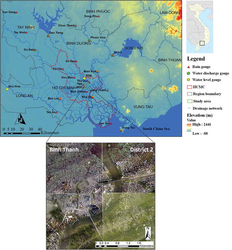
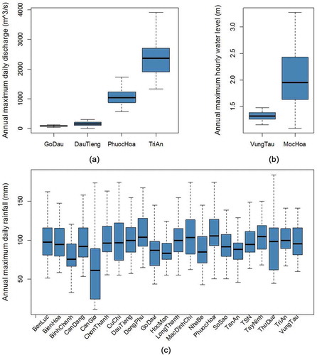
In addition, water discharge data from upstream areas was also collected and used in the frequency analysis. The daily water discharge data from Go Dau gauging station and three upstream reservoirs, i.e. Tri An, Dau Tieng and Phuoc Hoa, was provided by Trian Hydropower Joint Stock Company and Dau Tieng-Phuoc Hoa Limited Company for the period 1 January 1980 to 31 December 2014. For the Moc Hoa station, discharge data are not available; therefore, hourly water-level data provided by NHMS were used in this study. These data (i.e. water discharge and water level) were used for statistical analysis and to estimate return levels before being entered into the hydrodynamic model as upstream boundary conditions. Figure 2 shows the annual maximum daily discharge, annual maximum hourly water level and annual maximum daily rainfall at selected gauges in the Sai Gon–Dong Nai River basin.

Figure 2. Box plot of (a) annual maximum daily discharge, (b) annual maximum hourly water level and (c) annual maximum daily rainfall at selected gauges

2.2 Data for covariates

In this study, five physical covariates, namely ENSO, PDO, local mean temperature, global warming and global mean sea-level rise, were considered, to show the impacts of global and local processes on the nonstationarity of extreme events (i.e. rainfall, sea levels).

The ENSO cycle has had a significant impact at local and regional scales through teleconnections influencing the coupled ocean–atmosphere and land systems (Wang et al. 2006). The influences of this pattern on extreme rainfall and flooding have also been indicated in many parts of the world (e.g. Ishak et al. 2013, Li et al. 2015, Mondal and Mujumdar 2015, Villafuerte et al. 2015, Agilan and Umamahesh 2016, Gobin et al. 2016). In Vietnam, ENSO has been proven to play an important role in climate and to contribute to the inter-annual variation in rainfall in many regions (e.g. Yen et al. 2011, Nguyen et al. 2014, Gobin et al. 2016). In this study, monthly sea-surface temperature (SST) anomaly series over the Niño 3.4 region were used as ENSO indicator; these were obtained from the US National Oceanic and Atmospheric Administration (NOAA) Earth System Research Laboratory (ESRL).¹

The PDO, a pattern of Pacific climate variability, has been shown to have significant climatic and environmental impacts across the Pacific Basin (Deng et al. 2013). Together with ENSO, PDO has been investigated by many authors and found to have an influence on the East Asian monsoon, as well as seasonal rainfall patterns (Chan and Zhou 2005, Chen et al. 2013, Wu 2013). The PDO index was also extracted from NOAA ESRL,² and is used in the nonstationary frequency analysis as a covariate.

Increases in extreme rainfall have been documented in many regions across the world (IPCC, 2012) and human-influenced global warming may be partly responsible (Min et al. 2011). Kunkel et al. (2013) indicated that rising temperatures and subsequent rises in atmospheric moisture content might increase the probable maximum precipitation values. Nevertheless, the physical mechanisms linking local temperatures with rainfall may not be the same as those linking global warming to extreme rainfall changes (Trenberth 2011, Mondal and Mujumdar 2015). Therefore, global temperature and local temperatures are chosen as separate covariates for analysing the extreme rainfall characteristic in this study.

The HadCRUT4 annually observed global average surface air temperature anomaly series³ with respect to the 1961–1990 mean was used as an indicator of global warming. The yearly mean temperature data for the period 1980–2014 were provided by the Southern Institute for Water Resources Planning. These data were recorded at four stations located in HCMC: Tan Son Nhat (TSN), Bien Hoa, Dong Phu, Vung Tau, and three in adjacent regions (Fig. 1). The yearly mean temperature anomaly series based on the 1980–2014 mean was calculated and considered as a covariate.

In recent decades, extreme sea levels have been found to have increased in various regions worldwide (Woodworth et al. 2011). Many studies have reported that long-term changes in extreme sea levels are generally associated with corresponding increases in mean sea levels (Letetrel et al. 2010, Lowe et al. 2010, Feng and Tsimplis 2014, Weisse et al. 2014). As a coastal city, HCMC is expected to be severely influenced by sea-level rise. Hence, using global mean sea level as a covariate in extreme sea-level statistical analysis is reasonable. The global mean sea-level (GMSL) data used in this study are the up-to-date version of reconstructed GMSL from Church and White (2011) for the period 1980–2014.⁴

2.3 Soil, land use and DEM

Land use and land cover (LULC) maps, soil maps and 1-m resolution LiDAR data were used as input in the hydrological and hydrodynamic models. These data were provided by Ho Chi Minh City Department of Science and Technology and are not publicly available. The main types of soils in the Sai Gon Dong Nai River basin are alluvial, basalt, grey, black and soft soil. The main types of LULC in the study area are built-up areas, vegetation, bare soil and wetland. These data were used to estimate the parameters in the hydrological and hydrodynamic models.

3 Methodology

A flowchart of the proposed methodology for developing flood hazard maps is shown in Figure 3. The flowchart consists of four main sections. Apart from data preparation mentioned in Section 2, the three remaining sections are described as follows:

1. Annual maximum daily rainfall and hourly sea-level time series were used for frequency analysis. The generalized extreme value (GEV) distribution was chosen with the assumption of stationarity and nonstationarity in the time series. The magnitude of extreme rainfall from the best GEV model was used as input data for the hydrological model and, similarly, extreme sea level was used as the downstream boundary condition for the hydrodynamic model. Meanwhile, the values of upstream water level and discharge from the stationary GEV model were used as the upstream boundary conditions in the hydrodynamic model.

2. Estimation of runoff from sub-basins is based on the lumped conceptual rainfall–runoff model. The result from the rainfall–runoff model was used in 1D flow simulation.

3. Development of the 1D flow model, the 2D flow model and coupling of the 1D–2D models for the river system and identification of the spatial variation of flood hazards corresponding to three flood scenarios derived from a combination of extreme rainfall, sea levels and discharge for different return periods (i.e. 25, 50 and 100 years).

Figure 3. Proposed methodology flowchart for developing flood hazard maps

3.1 The generalized extreme value model

In this study, the GEV distribution, which has become a widely used method for block maxima, was used for the frequency analysis of extreme events. The cumulative distribution of the GEV is given by (Coles 2001, Katz 2013):

(1) $F\left(x;\mu ,\sigma ,\xi \right)=\left\{\begin{array}{c}\mathrm{e}\mathrm{x}\mathrm{p}\left\{-{\left[1+\xi \left(\frac{x-\mu }{\sigma }\right)\right]}^{-1/\xi }\right\},1+\xi \left(\frac{x-\mu }{\sigma }\right)>0,\sigma >0,\xi \ne 0\\ \mathrm{e}\mathrm{x}\mathrm{p}\left\{-\mathrm{e}\mathrm{x}\mathrm{p}\left[-\left(\frac{x-\mu }{\sigma }\right)\right]\right\},\sigma >0,\xi =0\end{array}\right.$(1)

where x is the independent value (e.g. rainfall, water level, discharge), while μ, σ and ζ are, respectively, the location, scale and shape parameters of the GEV distribution. Here, the nonstationarity is introduced in the location and scale parameters, whilst the shape parameter is kept constant because precise estimation of ξ is difficult, and it is unrealistic to assume that it is a smooth function of time (Coles 2001).

In the nonstationary setting, the parameters are expressed as a function of covariates in the general form:

Case 1: For extreme rainfall analysis

(2) $\begin{array}{c}\mu \left(t\right)={\mu }_0+{\mu }_{1}C\\ \sigma \left(t\right)=\mathrm{e}\mathrm{x}\mathrm{p}\left({\sigma }_0+{\sigma }_{1}C\right)\end{array}$(2)

Case 2: For extreme sea-level analysis

(3) $\begin{array}{c}\mu \left(t\right)={\mu }_0+{\mu }_{1}C\\ \sigma \left(t\right)=\mathrm{e}\mathrm{x}\mathrm{p}\left({\sigma }_0+{\sigma }_{1}C\right)\end{array}$(3)

Case 3: For extreme discharge and water-level analysis

(4) $\begin{array}{c}\mu \left(t\right)={\mu }_0\\ \sigma \left(t\right)={\sigma }_0\end{array}$(4)

where C represents any physical covariate, i.e. the ENSO cycle (E), PDO cycle (P), mean temperature anomaly (GT), local temperature (LT) or global sea-level rise (GS). In the stationary model (GEV-0), the values of C equal zero. The exponential in Equations (2)(2) $\begin{array}{c}\mu \left(t\right)={\mu }_0+{\mu }_{1}C\\ \sigma \left(t\right)=\mathrm{e}\mathrm{x}\mathrm{p}\left({\sigma }_0+{\sigma }_{1}C\right)\end{array}$(2) and (3(3) $\begin{array}{c}\mu \left(t\right)={\mu }_0+{\mu }_{1}C\\ \sigma \left(t\right)=\mathrm{e}\mathrm{x}\mathrm{p}\left({\sigma }_0+{\sigma }_{1}C\right)\end{array}$(3) ) is taken to ensure positive values of the scale parameter. Based on four covariates and their combinations, 25 nonstationary models were constructed for each raingauge in the extreme rainfall statistical analysis (details are given in the Supplementary material, Table S1). For extreme sea-level analysis 13 nonstationary models were constructed based on three covariates and their combinations (for only Vung Tau station) (details provided in Table S2). Based on these models, individual covariates or combinations that had significant impacts on the extreme rainfall and extreme sea levels in the study area were derived. In the case of extreme discharge and extreme water level from upstream, only the stationary condition was used for statistical analysis in this study (Equation (4)(4) $\begin{array}{c}\mu \left(t\right)={\mu }_0\\ \sigma \left(t\right)={\sigma }_0\end{array}$(4) ).

The method of maximum-likelihood was used for estimating the parameters of the GEV model in this study because it can easily be extended to the nonstationary case (Coles 2001). Let x₁, x₂, …, x_n be an annual maximum series of n years, with h the probability density function of the GEV distribution, and θ the vector of the parameters [θ = (µ(t), σ(t), ξ)]. The likelihood function can be written as:

(5) $L(\theta |X)={\prod }_{i=1}^{n}h\left(x_i,\theta \right)$(5)

Katz (2013) suggested that minimization of negative log-likelihood, for the purpose of optimization, could often be used to arrive at the estimates of parameters instead of maximization. Therefore, it was decided to adopt minimization of the negative log-likelihood function for estimating all parameters in this study.

Among multiple candidate models, the Akaike information criterion (AIC) has commonly been used to select appropriate models. However, Hurvich and Tsai (1995) showed that the AIC might have serious deficiencies; hence, they recommended a corrected version, namely AICc, which was developed for small samples to mitigate the bias and avoid overfitting the data. Thus, AICc was chosen for selecting the appropriate model, as given by:

(6) $\mathrm{A}\mathrm{I}\mathrm{C}\mathrm{c}=-2log\left(\mathrm{M}\mathrm{L}\right)+2m+\frac{2m\left(m+1\right)}{n-m-1}$(6)

where n is the sample size, m is the number of parameters in a given model, and −logL(θ|X) is the minimized negative log-likelihood function. In addition, Burnham and Anderson (2004) suggested a rescaled form of AICc, (denoted Δ_i), which was used for ranking the models, and is calculated as follows:

(7) ${\mathrm{\Delta }}_i=\mathrm{A}\mathrm{I}\mathrm{C}\mathrm{c}-\mathrm{A}\mathrm{I}\mathrm{C}{\mathrm{c}}_{\mathrm{m}\mathrm{i}\mathrm{n}}$(7)

where AICc_min is the smallest value of AICc, here regarding all candidate models. The model having Δ_i = 0 is considered as the best model and models that have Δ_i ≤ 2 are considered reasonable selections (Burnham and Anderson 2004).

Once the best model for extreme rainfall (or water level or discharge) is determined, the T-year return level z_T corresponding to the T-year return period can be obtained. Unlike in the stationary model, the location and scale parameters of the nonstationary model vary over time. Here we consider a low-risk approach (more conservative) suggested by Cheng et al. (2014), by taking the 95th percentiles of μ(t) and σ(t) in historical observations to calculate return levels in this study, as follows:

(8) ${\hat{\mu }}_{{ }_{95}}=Q_{95}({\hat{\mu }}_{{{ }_t}_1},{\hat{\mu }}_{{{ }_t}_2},...,{\hat{\mu }}_{{ }_{tn}})$(8)

(9) $\hat{\sigma }=Q_{95}\left({\sigma }_{{{ }_t}_1},{\sigma }_{{{ }_t}_2},...,{\sigma }_{{ }_{tn}}\right)$(9)

Estimation of the T-year return level can be given by (Coles 2001):

(10) $z_{T=}\left\{\begin{array}{c}\hat{\mu }-\frac{\hat{\sigma }}{\hat{\xi }}\left[1-{\left\{-\mathrm{l}\mathrm{o}\mathrm{g}\left(1-\frac{1}{T}\right)\right\}}^{-\hat{\xi }}\right]\mathrm{f}\mathrm{o}\mathrm{r}\hat{\xi }\ne 0\\ \hat{\mu }-\hat{\sigma }\mathrm{l}\mathrm{o}\mathrm{g}\left\{-\mathrm{l}\mathrm{o}\mathrm{g}\left(1-\frac{1}{T}\right)\right\}\mathrm{f}\mathrm{o}\mathrm{r}\hat{\xi }=0\end{array}\right.$(10)

By substituting the values of estimated parameters into Equation (10)(10) $z_{T=}\left\{\begin{array}{c}\hat{\mu }-\frac{\hat{\sigma }}{\hat{\xi }}\left[1-{\left\{-\mathrm{l}\mathrm{o}\mathrm{g}\left(1-\frac{1}{T}\right)\right\}}^{-\hat{\xi }}\right]\mathrm{f}\mathrm{o}\mathrm{r}\hat{\xi }\ne 0\\ \hat{\mu }-\hat{\sigma }\mathrm{l}\mathrm{o}\mathrm{g}\left\{-\mathrm{l}\mathrm{o}\mathrm{g}\left(1-\frac{1}{T}\right)\right\}\mathrm{f}\mathrm{o}\mathrm{r}\hat{\xi }=0\end{array}\right.$(10) , we obtained the estimates of the return levels.

3.2 Hydrological model

The lumped conceptual rainfall–runoff model is developed by conceptualizing the catchment as a number of interconnected storages, with a set of mathematical equations used to describe the process of the water flow lumped over them (Chiew 2010). Due to its simplicity, the lumped conceptual rainfall–runoff model has been widely used in previous studies to mimic hydrological processes in catchments (e.g. Madsen 2000, Anh et al. 2008, Brirhet and Benaabidate 2016). In this study, to estimate the generated runoff in the whole Sai Gon–Dong Nai River basin, it was divided into 216 sub-basins based on land topography. With 22 raingauges scattered throughout the sub-basins, the Thiessen polygons method was used as an interpolation method to calculate the average depth of rainfall on the area of these sub-basins. The storm runoff was estimated by the Soil Conservation Service (SCS) method (Hjelmfelt 1991), which is available in the MIKE 11 Unit Hydrograph Model (UHM) developed by the Danish Hydraulic Institute (DHI, 2003). The MIKE 11 UHM is a lumped conceptual rainfall–runoff model that simulates the runoff from a single rainstorm by using the unit hydrograph technique. The model runs on 24-h rainfall records and potential evaporation. For the flood scenarios, once the extreme rainfall is calculated through the best (non)stationary model for each station, this value is assumed to be uniformly distributed and used as input data for the rainfall–runoff model. The output from the rainfall–runoff model can be used as lateral inflow for the 1D hydrodynamic model.

3.3 Hydrodynamic model

In this study, the coupled 1D–2D model MIKE FLOOD was used to simulate the flood inundation for HCMC in the Sai Gon–Dong Nai River basin. The model was developed by the Danish Hydraulic Institute (DHI, 2007). To set up the 1D hydrodynamic model that represents the entire river system of the Sai Gon–Dong Nai River basin, the input data included cross-sections, Manning’s n roughness coefficients and boundary conditions. There are six boundaries. The hourly sea-level data (Vung Tau station) were used as the downstream boundary condition, while daily discharge time series from Tri An, Dau Tieng and Phuoc Hoa reservoirs, daily discharge data from Go Dau streamflow gauge located in the Vam Co Tay River, and hourly water level data from Moc Hoa water level gauge located in the Vam Co Dong River were used as upstream boundary conditions. Also, the five main rivers, i.e. Dong Nai, Sai Gon, Be, Vam Co Tay and Vam Co Dong, together with 251 small streams were established, and the details of 300 observed cross-sections were used in this study.

The 1D model (MIKE 11) was calibrated for the year 2012 and validated for the year 2011. In the calibration procedure, Manning’s roughness coefficient values were adjusted manually to produce the smallest deviations between the observed and modelled values. The initial Manning’s n values for channels were chosen from the study of Te Chow (1959). Ritter and Muñoz-Carpena (2013) suggested that, in the model performance assessment, one should include at least one absolute value error indicator, one dimensionless index and a graphical technique, which provide a visual comparison between observed data and model-calculated values.

In this study, the following statistical criteria were used to assess model performance: the coefficient of determination (R²), the ratio of root mean square error to standard deviation observations (RSR), the Nash-Sutcliffe efficiency (NSE; Nash and Sutcliffe 1970), and a graphical representation of the relationship between observations and model estimates. The R² describes the proportion of the variance in measured data explained by the model, where R² = 1 is considered as the perfect match, and values greater than 0.5 are acceptable (Moriasi et al. 2007, Jeong et al. 2010). The RSR incorporates the benefits of error index statistics and includes a normalization factor, so that the resulting statistic can apply to various constituents (Moriasi et al. 2007). Values of RSR range from the optimal value of 0 to a large positive value. The NSE, ranging between $-\mathrm{\infty }$and 1.0, is commonly used to access the predictive power of the model (Nguyen et al. 2016). Normally, NSE of 0.65 is considered good for daily results. However, the criteria may be lower for sub-daily outputs and higher for monthly and annual outputs, since performance improves as the time interval increases (Jeong et al. 2010). The RSR and NSE are calculated as follows:

(11) $\mathrm{R}\mathrm{S}\mathrm{R}=\frac{\sqrt{{\sum }_{i=1}^N{\left(X_i^{\mathrm{o}\mathrm{b}\mathrm{s}}-X_i^{\mathrm{s}\mathrm{i}\mathrm{m}}\right)}^2}}{\sqrt{{\sum }_{i=1}^N{\left(X_i^{\mathrm{o}\mathrm{b}\mathrm{s}}-X^{{ }^{\mathrm{m}\mathrm{e}\mathrm{a}\mathrm{n}}}\right)}^2}}$(11)

(12) $\mathrm{N}\mathrm{S}\mathrm{E}=1-\frac{{\sum }_{i=1}^N{\left(X_i^{\mathrm{o}\mathrm{b}\mathrm{s}}-X_i^{\mathrm{s}\mathrm{i}\mathrm{m}}\right)}^2}{{\sum }_{i=1}^N{\left(X_i^{\mathrm{o}\mathrm{b}\mathrm{s}}-X^{{ }^{\mathrm{m}\mathrm{e}\mathrm{a}\mathrm{n}}}\right)}^2}$(12)

where $X_i^{\mathrm{o}\mathrm{b}\mathrm{s}}$ and $X_i^{\mathrm{s}\mathrm{i}\mathrm{m}}$ are the ith observed and simulated data, $X^{\mathrm{m}\mathrm{e}\mathrm{a}\mathrm{n}}$ is the mean of observed data, and N is the total number of observations.

The developed 2D model comprises a flexible mesh with 686 173 elements and 343 498 nodes, which covers the study area (16 km²) mentioned in Section 3.5. Manning’s n values for floodplain areas are referred to in Timbadiya et al. (2014). In particular, Manning’s n values for the residential areas, agriculture areas and water bodies are 0.2, 0.07 and 0.03, respectively. The surface elevations for the study area were derived from 1-m resolution LiDAR data. Due to the lack of detailed historical data for inundation events, calibration and validation for the 2D model was not carried out.

3.4 Flood scenario simulations

Three sets of model simulations were carried out for different flood scenarios derived from a combination of extreme rainfall, sea levels and discharge, as shown in Table 1. For the upstream boundary conditions in each scenario, the estimated daily discharge from the frequency analysis (Tri An, Dau Tieng, Phuoc Hoa and Go Dau) was assumed to be at a constant value. Similarly, the only upstream boundary condition in the Vam Co Dong River was assigned as estimated water level (Moc Hoa), which is considered as constant. For the downstream boundary, we used hourly sea-level time series from 24 December 1999, when the highest water level station was recorded at Vung Tau. The observed hourly sea levels were then amplified until the tidal peak matched the value of extreme sea level gained from the best GEV model. The hourly sea-level time series after amplifying were used as downstream boundary conditions for the hydrodynamic model. It is to be noted that the impacts of waves were not considered.

Table 1. Initial model inputs for the three scenarios investigated (i.e. 25-, 50- and 100-year return periods)

	Return period (years)
Model simulation	Rainfall	Sea level	Discharge
Scenario 1	25	25	25
Scenario 2	50	50	50
Scenario 3	100	100	100

3.5 Case study

Located in the downstream of the Sai Gon–Dong Nai River systems, the topographical and geographical conditions of HCMC make it extremely sensitive to various flood sources. The city is subject to both regular and extreme flooding. In 2050, 61% of urban land use and 67% of industrial land use are expected to be flooded in an extreme event if the proposed flood control measures are not implemented (World Bank 2010). However, generating detailed flood hazard maps based on high-resolution topographical data for the whole of HCMC, which covers a very large area (approx. 2095 km²), requires high computational resources. Our study is limited to the area located close to the Saigon River branch, a distributary of the Sai Gon–Dong Nai River system, covering an area of 16 km². This area belongs to Binh Thanh district and District 2 (Fig. 1), and is an example of low-lying lands that are prone to frequent flooding caused by high tide, heavy rainfall and high water discharge released from the upstream reaches of the river basin. Binh Thanh district represents an urban district with a very high population density, while District 2 represents a semi-urban district, and is considered to become the most strategic metropolitan area in HCMC in the near future. District 2 and Binh Thanh district are estimated to be severely impacted by extreme floods in 2050, with approximately 94 and 82% of their area flooded, respectively (World Bank 2010). The main land use in this area is residential buildings (i.e. built-up land), intermingled with a few areas of fallow lands. The width of the Saigon River in this area varies between 250 and 350 m, while its average depth is about 20 m.

3.6 Flood hazard classification

Flood hazard maps provide essential information for flood risk management and mitigation purposes. In most flood hazard studies, flood-water depth is widely used to classify a hazard index (e.g. Alfieri et al. 2014, Garrote et al. 2016, Sharif et al. 2016, Komi et al. 2017). Nevertheless, flood hazard includes many elements, such as the stability of human bodies, buildings and vehicles in flood waters (Xia et al. 2011). Therefore, a single parameter cannot completely assess the potential damage due to flood flows on people, buildings and vehicles. In previous studies, a combination of flood depth (D) and velocity (V) has been used as a proxy for the force of flood waters to access the instability of the human body and vehicles, as well as the failure of buildings in flood waters (Kreibich et al. 2009, Xia et al. 2011, 2014). Furthermore, Smith et al. (2014) and AEMI (2014) indicated that the level of vulnerability of a community is dependent on the strength of the flood waters, which can be simply described by the depth and speed of flood waters. They also suggested that flood hazard maps may be classified using combined flood hazard curves derived from flood depth and velocity thresholds. This method provides a basis for categorizing flood hazard based on the intensity of D × V, and it was used in this study. As such, the classification of flood hazard was based on a six-grade scale, ranging from H1 to H6. The class H1 represents a very low hazard, which is generally safe for people, vehicles and buildings, whereas H6 is unsafe for people, vehicles and buildings. The flood hazard classification limits (AEMI, 2014) are presented in Table 2. For further details about flood hazard classification, the reader is referred to Smith et al. (2014) and AEMI (Australia Emergency Management Institute) (2014).

Table 2. Limits for the flood hazard classification

Hazard class	Flood depth, D(m)	Velocity, V(m/s)	Classification limit (D × V) (m^2/s)	Description
H1	0.3	2.0	≤0.3	Generally safe for vehicles, people and buildings
H2	0.5	2.0	≤0.6	Unsafe for small vehicles
H3	1.2	2.0	≤0.6	Unsafe for vehicles, children and the elderly
H4	2.0	2.0	≤ 1.0	Unsafe for vehicles and people
H5	4.0	4.0	≤4.0	Unsafe for vehicles and people; all building types vulnerable to structural damage
H6	-	-	>4.0	Unsafe for vehicles and people; all buildings types vulnerable to failure

4 Results and discussion

4.1 Frequency analysis

The best GEV models were fitted to annual maximum rainfall, annual maximum water level and annual maximum discharge for all gauging stations, and the results are presented in Table 3, which also shows the parameter values of appropriate GEV models from the results of frequency analysis. The models with lower AICc should be preferred to those with higher AICc, and the best model is identified as the model with Δ_i equal to zero.

Table 3. Results of the best GEV models and parameter estimation. The best model for each station is based on the lowest value of the AICc

Station	Model	µ0	µ1	µ2	µ3	σ0	σ1	σ2	ξ	Δi *
Rainfall
Ben Luc	GEV-2	90.98	−9.66	-	-	22.47	-	-	0.17	1.50
Bien Hoa	GEV-0	86.43	-	-	-	21.56	-	-	0.10	-
Binh Chanh	GEV-1	68.67	−12.27	-	-	17.51	-	-	0.31	3.25
Can Dang	GEV-0	85.45	-	-	-	21.86	-	-	0.05	-
Can Gio	GEV-7	44.00	−10.81	45.15	-	20.83	-	-	0.35	14.12
Chon Thanh	GEV-0	90.56	-	-	-	23.30	-	-	0.05	-
Cu Chi	GEV-1	84.78	−19.00	-	-	21.86	-	-	0.14	4.48
Dau Tieng	GEV-0	90.26	-	-	-	22.14	-	-	0.13	-
Dong Phu	GEV-0	97.41	-	-	-	25.31	-	-	0.26	-
Go Dau	GEV-4	75.88	−12.30	-	-	20.41	-	-	−0.18	0.39
Hoc Mon	GEV-0	77.74	-	-	-	22.93	-	-	−0.22	-
Long Thanh	GEV-5	92.31	16.16	-	-	23.52	-	-	0.22	2.71
Mac Dinh Chi	GEV-3	102.38	−35.12	-	-	21.43	-	-	0.02	0.02
Nha Be	GEV-20	77.85	3.65	−5.30	-	3.32	1.28	−0.79	−0.27	4.20
Phuoc Hoa	GEV-0	95.87	-	-	-	29.05	-	-	0.10	-
So Sao	GEV-0	87.15	-	-	-	21.31	-	-	−0.10	-
Tan An	GEV-23	84.12	−15.28	−21.93	-	2.88	0.72	−1.24	0.32	12.61
Tay Ninh	GEV-2	94.78	−6.91	-	-	17.86	-	-	0.28	1.31
Thu Duc	GEV-10	130.55	−174.18	59.32	-	21.34	-	-	0.26	3.33
Tri An	GEV-0	91.65	-	-	-	17.45	-	-	−0.02	-
TSN	GEV-12	88.20	15.37	−6.68	−18.58	13.17	-	-	0.34	2.83
Vung Tau	GEV-0	86.17	-	-	-	22.65	-	-	0.31	-
Water level
Vung Tau	GEV-3	1.24	0.002	-	-	0.06	-	-	−0.03	10.07
Moc Hoa	GEV-0	1.82	-	-	-	0.47	-	-	−0.16	-
Discharge
Go Dau	GEV-0	69.83	-	-	-	22.79	-	-	−0.10	-
Dau Tieng	GEV-0	113.72	-	-	-	97.73	-	-	0.18	-
Phuoc Hoa	GEV-0	949.74	-	-	-	263.06	-	-	−0.11	-
Tri An	GEV-0	2091.25	-	-	-	500.60	-	-	−0.09	-

*Denotes Δ_i between the best model and GEV-0.

The results presented in Table 3 show that the nonstationary GEV models are superior to the stationary GEV models at 12 of the 22 stations studied, while there was no evidence of nonstationarity at the remaining rainfall stations. Taking TSN station as an example, the GEV-12 model was found to be the best model for extreme rainfall based on Δ_i. In the GEV-12 model, the linear trend is represented by the location parameter with three covariates of ENSO, PDO and local temperature, with a value of Δ_i between GEV-0 and GEV-12 of 2.83.

For Vung Tau station (sea level), the GEV-3 model that considered global sea-level rise as a covariate was found to be the best model. The stationary model is ranked eight among the 15 models, and the value of Δ_i for GEV-3 was 10.07.

The discharge time series at Go Dau, Dau Tieng, Phuoc Hoa and Tri An stations and the water level time series at Moc Hoa were assumed to be under stationary conditions, and the maximum-likelihood estimates for location, scale and shape parameters in the stationary models for these stations are also given in Table 3.

Based on the best models, the estimated values of rainfall, sea/water level and discharge corresponding to return periods of 2, 5, 10, 25, 50 and 100 years are provided in Table 4. It can be seen from Table 4 that there is a huge difference in the magnitudes of extreme rainfall between gauging stations in the surveyed basin. For example, the extreme rainfall for the 100-year return period at Hoc Mon station is even lower than the 5-year return period value at Tan An station. Three flood scenarios based on the values of rainfall, sea/water level and discharge corresponding 25-, 50- and 100-year return periods, presented in Table 4, were used in flood simulation.

Table 4. Variation in return levels for different return periods

Station	Return period (years)
	2	5	10	25	50	100
Rainfall (mm)
Ben Luc	110.54	140.51	163.83	197.94	227.11	259.78
Bien Hoa	94.48	121.31	140.83	167.67	189.29	212.31
Binh Chanh	86.00	112.72	136.43	175.56	213.10	259.51
Can Dang	93.54	119.54	137.61	161.46	179.91	198.91
Can Gio	107.24	140.17	170.37	221.81	272.64	337.11
Chon Thanh	99.18	126.86	146.08	171.42	191.01	211.16
Cu Chi	110.53	138.79	160.13	190.52	215.81	243.51
Dau Tieng	98.57	126.93	148.15	178.10	202.83	229.73
Dong Phu	107.14	143.86	174.87	223.81	268.78	322.37
Go Dau	92.14	111.79	122.80	134.78	142.46	149.20
Hoc Mon	85.82	107.12	118.61	130.70	138.19	144.59
Long Thanh	116.97	149.80	176.52	217.24	253.46	295.40
Mac Dinh Chi (MDC)	110.27	135.04	151.78	173.30	189.55	205.92
Nha Be	105.61	164.81	195.11	225.54	243.57	258.37
Phuoc Hoa	106.72	142.98	169.40	205.84	235.26	266.64
So Sao	94.82	116.87	130.17	145.64	156.22	166.03
Tan An	110.23	176.09	234.99	332.99	427.69	545.52
Tay Ninh	109.59	135.98	158.69	195.12	229.14	270.24
Thu Duc	109.54	140.58	166.86	208.42	246.70	292.40
Tri An	98.02	117.37	129.91	145.44	156.74	167.78
TSN	106.87	127.42	146.02	177.33	207.91	246.32
Vung Tau	94.96	129.51	160.11	210.59	258.97	318.75
Water level (m)
Vung Tau	1.40	1.47	1.51	1.56	1.60	1.64
Moc Hoa	1.99	2.45	2.72	3.01	3.20	3.37
Discharge (m^3/s)
Go Dau	78.03	101.55	115.71	132.14	143.35	153.72
Dau Tieng	150.74	281.86	384.51	535.57	665.41	811.51
Phuoc Hoa	1044.26	1313.85	1474.94	1660.57	1786.44	1902.23
Tri An	2271.68	2792.79	3109.19	3479.07	3733.43	3970.20

4.2 Model calibration and validation

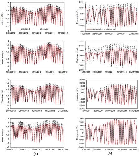
The hourly water level data for the rainy period (1–24 September 2012) at four gauging stations (Ben Luc, Bien Hoa, Nha Be, TDM) were used to calibrate the hydrodynamic model. The results of the simulations are presented in Table 5. It may be seen that the RSR for hourly water levels varies from 0.32 to 0.66, while R² values vary from 0.88 to 0.97. The hourly NSE values range between 0.61 and 0.89, with an average value of 0.71.

Table 5. Calibration and validation results: 1D model

Station	Calibration (hourly water level)			Validation (hourly water discharge)
	R^2	RSR	NSE	R^2	RSR	NSE
Ben Luc	0.97	0.55	0.7	0.91	0.4	0.84
Bien Hoa	0.88	0.66	0.61	0.77	0.7	0.51
Nha Be	0.96	0.32	0.89	0.81	0.65	0.58
TDM	0.97	0.59	0.65	0.93	0.42	0.82

Validation of the model was performed using hourly discharge data for the period 19 September to 4 October 2011. The model performance at Ben Luc and TDM stations was good, with NSE values of 0.84 and 0.82, respectively (Table 5), while the NSE values for Bien Hoa and Nha Be were much lower (0.51 and 0.58, respectively).

Figure 4 shows the comparison of observed and simulated hourly water levels under calibration (Fig. 4(a)) as well as hourly discharge under validation (Fig. 4(b)). There is a good level of agreement between the observed and simulated water levels and discharges at all the gauging stations. Therefore, the model can be used appropriately for the subsequent simulation.

Figure 4. Results of (a) calibration and (b) validation of the flood simulation model at, from top to bottom, Ben Luc, Bien Hoa, Nha Be and TDM stations

4.3 Flood hazard map

Based on the developed model, the flood hazard maps derived from the combination of extreme rainfall, water levels and upstream outflows are presented in Figure 5. The maps represent three different scenarios, 1, 2 and 3 for 25-, 50- and 100-year return periods, respectively. The enlarged views are shown in Figure 6(a)–(c), focusing on the large flooded areas (denoted by A1, A2 and A3). It can be seen that areas where the river is surrounded by houses and buildings, or where the riverbed is narrow, the flood inundation extent is wider. Taking a closer look at areas A1, A2 and A3, the flood water flows freely over the riverbank along roads and alleyways.

Figure 5. Comparison of flood hazard maps between flood scenarios, with return periods of (a) 25, (b) 50 and (c) 100 years. Flood hazard is classified by considering the combination of flood depth and velocity, ranging from H1 to H6 (see Table 2)

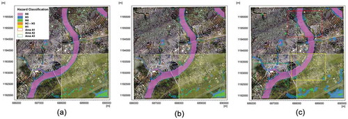
Figure 6. Enlarged view of areas A1, A2 and A3 (Fig. 5) for different flood scenarios, with return periods of (a) 25, (b) 50 and (c) 100 years. (d) Area of each flood hazard zone corresponding to each flood scenario

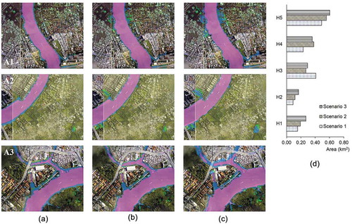
The flood hazard is classified based on six levels (Section 3.6, Table 2), and the area of each flood hazard zone in relation to the entire study area is presented in Figure 6(d). However, as the area of the H6 flood hazard zone mostly covers the main river surface, it is not shown in Figure 6(d). It is clear that the total flooded area increases corresponding to flood events. In particular, the H1 flood hazard zone, which is generally safe for all people, vehicles and infrastructure, covers areas of 0.15, 0.19 and 0.27 km² under scenarios 1, 2 and 3, respectively. The cumulative area of the H2, H3 and H4 flood hazard zones, where the water depth varies from 0.5 to 2.0 m under Scenario 1, is 0.73 km², while for scenarios 2 and 3, the corresponding areas are 0.77 and 0.82 km², respectively. Finally, the H5 flood hazard zone, which is unsafe for people, vehicles and buildings, covers 0.49, 0.56 and 0.60 km² under scenarios 1, 2 and 3, respectively.

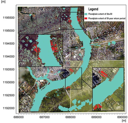
Furthermore, a floodplain map based on the combination of 50-year extreme rainfall, extreme sea level and extreme discharge under stationary conditions (denoted Sta-50) was developed for comparison purposes and is shown in Figure 7. It can be seen that the flood extent under nonstationary conditions is larger than under stationary conditions. The flooded area under Scenario 2 is 0.29 km² larger than that under Sta-50. The enlarged views (Fig. 7(a) and (b)) show two areas in which the difference in flooded area between the two scenarios (Scenario 2 and Sta-50) is particularly remarkable.

Figure 7. Comparison of floodplain extents of 50-year return period and Sta-50, with (a) and (b) showing zoomed-in images of the flooded areas. Sta-50: 50-year extreme rainfall, extreme sea level and extreme discharge under stationary conditions

The results demonstrate how flood potential can influence human settlements in the study area. Compared to the flood simulation methods used in previous studies (Lasage et al. 2014, Dang and Kumar 2017), the current method has applicability in flood simulation when considering the nonstationary behaviour in time series of extreme events. In comparison with Storch and Downes (2011), ADB (2010) and (World Bank 2010), our results show that the flooded areas are discrete and concentrated mainly on both sides of the Saigon River rather than covering the entire study area. More importantly, the high-resolution images from our study provide a clear and detailed view of the flooded area, which can contribute to efficient flood risk management, as well as provision of mitigation strategies by local government.

5 Summary and conclusions

One of the key factors in preventing and reducing flood damage and the number of lives lost is the provision of flood risk assessment information through flood hazard maps. In HCMC, extreme rainfall and extreme sea levels are considered as the main factors impacting significantly on floodplain extent. These factors are currently proven to have nonstationarity in their time series. We believe that ours is the first study to develop a flood simulation model considering nonstationarity in two time series of flood components, i.e. extreme rainfall and extreme sea levels; this is different from other research on flooding in HCMC. Moreover, the effect of upstream outflows on flood inundation in HCMC was also considered, which contributed to the model development process. For this purpose, climate indices (ENSO, PDO), global and local temperature, and global mean sea level were used for frequency analysis to investigate the nonstationarity in the extreme rainfall and sea levels. The covariates in the best statistical model were attributed as the most significant physical processes causing nonstationarity in the time series. The results of frequency analysis show that ENSO and PDO are present in the best nonstationary models, hence they can be considered as the main causes of nonstationary behaviour in extreme rainfall in the study area. Another finding indicates that global sea-level rise has a significant effect on nonstationarity in extreme sea levels at Vung Tau station.

Flood scenarios were developed based on the results of frequency analysis corresponding to 25-, 50- and 100-year return periods. The calibration and validation results of the MIKE FLOOD model show that the model performs satisfactorily in simulating water flow for the study area. Another notable highlight in this paper is the use of high-resolution data (LiDAR) in developing the flood hazard maps of HCMC, which has not been done in previous studies. In this way, floodplain extent can be defined, and the passage of flood water can be detected clearly, even at the scale of street networks. The results from the spatial variation of flood hazards indicate that locations along both riverbanks are expected to experience a significant increase in flooded area, with the intensity of DV reaching 4.0 m²/s. The percentages of flooded area classified as zones H1–H5 are 8.54, 9.43 and 10.51% for scenarios 1, 2 and 3, respectively. It is also to be noted that the floodplain extent is larger when based on the assumption of nonstationarity.

Considering the important role of flood hazard mapping and estimating floodplain extent in decision making, or establishing flood warning systems, it is suggested that the flood components (e.g. rainfall, water level, upstream outflow, sea-level rise) are analysed under both stationary and nonstationary conditions before being used as initial inputs of hydrological and hydrodynamic models, since the global climate is continuously changing and unpredictable. The present work has successfully introduced nonstationarity into flood frequency analysis, thereby influencing the appearance of flood hazard maps. Nevertheless, several limitations have to be acknowledged. First, the use of 35 years of data might raise concerns about the uncertainty associated with parameter estimation, hence impacts on the extreme value estimates. Second, the missing calibration and validation of the 2D model might lead to an imperfect flood simulation model. However, it could be a suitable option for flood simulation in HCMC, since data are not available for a longer duration in this large river basin. The study provides a new approach for flood simulation in HCMC that can be referred to by managers and decision makers, especially for purposes relating to the construction of buildings and infrastructure in flood hazard areas. Moreover, the proposed flood simulation model may be used not only for HCMC but also for other practical cases within the Sai Gon–Dong Nai River basin, where insufficient attention has been paid to detailed flood maps.

Uncertainty analysis is considered as an important part of the flood modelling process. In the literature, sources of uncertainty are described as consisting of natural and epistemic uncertainty (Merz and Thieken 2005). Natural uncertainty is due to the variability of the underlying stochastic process, while epistemic uncertainty is related to lack of knowledge, subjective uncertainty, measurement errors, sampling variability and model errors. Identifying and quantifying uncertainty was not within the scope of this study, but this may be pursued in future work.

Acknowledgments

The authors are grateful to the National Hydro-Meteorological Service (NHMS) of Vietnam, Ho Chi Minh City Department of Science and Technology, Trian Hydropower Joint Stock Company and Dau Tieng–Phuoc Hoa Limited Company for providing long-term rainfall, water-level, sea-level and discharge data, soil maps, land use and land cover maps, and LiDAR data for this study.

Disclosure statement

No potential conflict of interest was reported by the authors.

Supplementary material

Supplemental data for this article can be accessed here.

Notes

¹ https://www.esrl.noaa.gov/psd/gcos_wgsp/Timeseries/Nino34/.

² https://www.esrl.noaa.gov/psd/data/climateindices/list/.

³ http://www.metoffice.gov.uk/hadobs/hadcrut4/.

⁴ http://www.cmar.csiro.au/sealevel/sl_data_cmar.html.

References

- ADB (Asian Development Bank), 2010. Ho Chi Minh City Adaptation to Climate Change: summary report [Online]. Asian Development Bank. Available from: https://www.adb.org/publications/ho-chi-minh-city-adaptation-climate-change-summary-report [ Accessed 19 Dec 2016].
- AEMI (Australia Emergency Management Institute), 2014. Technical flood risk management guideline: flood hazard. Australia: Australia Emergency Management Institute.
- Agilan, V. and Umamahesh, N., 2016. What are the best covariates for developing non-stationary rainfall intensity-duration-frequency Relationship?. Advances in Water Resources, 101, 11–22.
- Alfieri, L., et al., 2014. Advances in pan-European flood hazard mapping. Hydrological Processes, 28, 4067–4077. doi:10.1002/hyp.v28.13
- Anh, N.L., et al., 2008. An evaluation of three lumped conceptual rainfall–runoff models at catchment scale. Sheffield, UK: The 13th World Water Congress.
- Bates, P.D., et al., 2005. Simplified two-dimensional numerical modelling of coastal flooding and example applications. Coastal Engineering, 52, 793–810. doi:10.1016/j.coastaleng.2005.06.001
- Binh, L.T.H., et al., 2018. Modeling Nonstationary Extreme Water Levels Considering Local Covariates in Ho Chi Minh City, Vietnam. Journal of Hydrologic Engineering, 23, 04018042. doi:10.1061/(ASCE)HE.1943-5584.0001697
- Brirhet, H. and Benaabidate, L., 2016. Comparison Of Two Hydrological Models (Lumped And Distributed) Over A Pilot Area Of The Issen Watershed In The Souss Basin, Morocco. European Scientific Journal, ESJ, 12. doi:10.19044/esj.2016.v12n18p347
- Burnham, K.P. and Anderson, D.R., 2004. Multimodel inference understanding AIC and BIC in model selection. Sociological Methods & Research, 33, 261–304. doi:10.1177/0049124104268644
- Chan, J.C. and Zhou, W., 2005. PDO, ENSO and the early summer monsoon rainfall over south China. Geophysical Research Letters, 32. doi:10.1029/2004GL022015
- Chen, W., Feng, J., and Wu, R., 2013. Roles of ENSO and PDO in the link of the East Asian winter monsoon to the following summer monsoon. Journal of Climate, 26, 622–635. doi:10.1175/JCLI-D-12-00021.1
- Cheng, L., et al., 2014. Non-stationary extreme value analysis in a changing climate. Climatic Change, 127, 353–369. doi:10.1007/s10584-014-1254-5
- Chiew, F.H., 2010. Lumped conceptual rainfall–runoff models and simple water balance methods: overview and applications in ungauged and data limited regions. Geography Compass, 4, 206–225. doi:10.1111/j.1749-8198.2009.00318.x
- Church, J.A. and White, N.J., 2011. Sea-level rise from the late 19th to the early 21st century. Surveys in Geophysics, 32, 585–602. doi:10.1007/s10712-011-9119-1
- Coles, S., 2001. An introduction to statistical modeling of extreme values. London: Springer.
- Dang, A.T.N. and Kumar, L., 2017. Application of remote sensing and GIS-based hydrological modelling for flood risk analysis: a case study of District 8, Ho Chi Minh city, Vietnam. Geomatics, Natural Hazards and Risk, 8 (2), 1792–1811. doi:10.1080/19475705.2017.1388853
- Dasgupta, S., et al., 2011. Exposure of developing countries to sea-level rise and storm surges. Climatic Change, 106, 567–579. doi:10.1007/s10584-010-9959-6
- Delgado, J.M., Apel, H., and Merz, B., 2010. Flood trends and variability in the Mekong river. Hydrology and Earth System Sciences, 14, 407–418. doi:10.5194/hess-14-407-2010
- Deng, W., et al., 2013. Variations in the Pacific Decadal Oscillation since 1853 in a coral record from the northern South China Sea. Journal of Geophysical Research: Oceans, 118, 2358–2366.
- DHI (Danish Hydraulic Institute), 2003. MIKE11-A modelling system for Rivers and Channels. Denmark: Danish Hydraulic Institute.
- DHI (Danish Hydraulic Institute), 2007. MIKE FLOOD. Denmark: Danish Hydraulic Institute.
- Feng, X. and Tsimplis, M.N., 2014. Sea level extremes at the coasts of China. Journal of Geophysical Research: Oceans, 119, 1593–1608.
- Garrote, J., Alvarenga, F., and Díez-Herrero, A., 2016. Quantification of flash flood economic risk using ultra-detailed stage–damage functions and 2-D hydraulic models. Journal of Hydrology, 541, 611–625. doi:10.1016/j.jhydrol.2016.02.006
- Ghostine, R., et al., 2015. Comparison between a coupled 1D-2D model and a fully 2D model for supercritical flow simulation in crossroads. Journal of Hydraulic Research, 53, 274–281. doi:10.1080/00221686.2014.974081
- Gilroy, K.L. and Mccuen, R.H., 2012. A nonstationary flood frequency analysis method to adjust for future climate change and urbanization. Journal of Hydrology, 414-415, 40–48. doi:10.1016/j.jhydrol.2011.10.009
- Gobin, A., et al., 2016. Heavy rainfall patterns in Vietnam and their relation with ENSO cycles. International Journal of Climatology, 36, 1686–1699. doi:10.1002/joc.2016.36.issue-4
- Hallegatte, S., et al., 2013. Future flood losses in major coastal cities. Nature Climate Change, 3, 802–806. doi:10.1038/nclimate1979
- Hanson, S., et al., 2011. A global ranking of port cities with high exposure to climate extremes. Climatic Change, 104, 89–111. doi:10.1007/s10584-010-9977-4
- Hjelmfelt, A.T., Jr., 1991. Investigation of curve number procedure. Journal of Hydraulic Engineering, 117, 725–737. doi:10.1061/(ASCE)0733-9429(1991)117:6(725)
- Hurvich, C.M. and Tsai, C.-L., 1995. Model selection for extended quasi-likelihood models in small samples. Biometrics, 51, 1077–1084. doi:10.2307/2533006
- IPCC (Intergovernmental Panel on Climate Change), 2012. Managing the risks of extreme events and disasters to advance climate change adaptation. Special report of the Intergovernmental Panel on Climate Change. Cambridge, UK: Cambridge University Press.
- Ishak, E., et al., 2013. Evaluating the non-stationarity of Australian annual maximum flood. Journal of Hydrology, 494, 134–145. doi:10.1016/j.jhydrol.2013.04.021
- Jeong, J., et al., 2010. Development and integration of sub-hourly rainfall–runoff modeling capability within a watershed model. Water Resources Management, 24, 4505–4527. doi:10.1007/s11269-010-9670-4
- Jongman, B., Ward, P.J., and Aerts, J.C., 2012. Global exposure to river and coastal flooding: long term trends and changes. Global Environmental Change, 22, 823–835. doi:10.1016/j.gloenvcha.2012.07.004
- Karamouz, M., Ahmadvand, F., and Zahmatkesh, Z., 2017. Distributed Hydrologic Modeling of Coastal Flood Inundation and Damage: nonstationary Approach. Journal of Irrigation and Drainage Engineering, 143, 04017019. doi:10.1061/(ASCE)IR.1943-4774.0001173
- Katz, R.W., 2013. Statistical methods for nonstationary extremes. Extremes in a Changing Climate. Dordrecht: Springer.
- Komi, K., et al., 2017. Modelling of flood hazard extent in data sparse areas: a case study of the Oti River basin, West Africa. Journal of Hydrology: Regional Studies, 10, 122–132.
- Kreibich, H., et al., 2009. Is flow velocity a significant parameter in flood damage modelling?. Natural Hazards and Earth System Sciences, 9, 1679–1692. doi:10.5194/nhess-9-1679-2009
- Kunkel, K.E., et al., 2013. Probable maximum precipitation and climate change. Geophysical Research Letters, 40, 1402–1408. doi:10.1002/grl.50334
- Lasage, R., et al., 2014. Assessment of the effectiveness of flood adaptation strategies for HCMC. Natural Hazards and Earth System Sciences, 14, 1441–1457. doi:10.5194/nhess-14-1441-2014
- Leandro, J., et al., 2009. Comparison of 1D/1D and 1D/2D coupled (sewer/surface) hydraulic models for urban flood simulation. Journal of Hydraulic Engineering, 135, 495–504. doi:10.1061/(ASCE)HY.1943-7900.0000037
- Letetrel, C., et al., 2010. Sea level extremes in Marseille (NW Mediterranean) during 1885–2008. Continental Shelf Research, 30, 1267–1274. doi:10.1016/j.csr.2010.04.003
- Li, J., Liu, X., and Chen, F., 2015. Evaluation of nonstationarity in annual maximum flood series and the associations with large-scale climate patterns and human activities. Water Resources Management, 29, 1653–1668. doi:10.1007/s11269-014-0900-z
- López, J. and Francés, F., 2013. Non-stationary flood frequency analysis in continental Spanish rivers, using climate and reservoir indices as external covariates. Hydrology and Earth System Sciences, 17, 3189–3203. doi:10.5194/hess-17-3189-2013
- Lowe, J.A., et al., 2010. Past and future changes in extreme sea levels and waves. In: Church, J. A., Woodworth, P. L., Aarup, T. & Wilson, W. S. eds. Understanding sea-level rise and variability. UK: Wiley-Blackwell, 326–375.
- Machado, M.J., et al., 2015. Flood frequency analysis of historical flood data under stationary and non-stationary modelling. Hydrology and Earth System Sciences, 19, 2561–2576. doi:10.5194/hess-19-2561-2015
- Madsen, H., 2000. Automatic calibration of a conceptual rainfall–runoff model using multiple objectives. Journal of Hydrology, 235, 276–288. doi:10.1016/S0022-1694(00)00279-1
- Merz, B. and Thieken, A.H., 2005. Separating natural and epistemic uncertainty in flood frequency analysis. Journal of Hydrology, 309, 114–132. doi:10.1016/j.jhydrol.2004.11.015
- Milly, P.C., et al., 2008. Stationarity is dead: whither water management?. Science, 319, 573–574. doi:10.1126/science.1151915
- Min, S.-K., et al., 2011. Human contribution to more-intense precipitation extremes. Nature, 470, 378–381. doi:10.1038/nature09763
- Minh, N.H., et al., 2007. Persistent organic pollutants in sediments from Sai Gon–dong Nai river Basin, Vietnam: levels and temporal trends. Archives of Environmental Contamination and Toxicology, 52, 458–465. doi:10.1007/s00244-006-0157-5
- Mondal, A. and Mujumdar, P.P., 2015. Modeling non-stationarity in intensity, duration and frequency of extreme rainfall over India. Journal of Hydrology, 521, 217–231. doi:10.1016/j.jhydrol.2014.11.071
- Moore, M.R., 2011. Development of a high-resolution 1D/2D coupled flood simulation of Charles City, Iowa. Master Thesis. University of Iowa.
- Moriasi, D.N., et al., 2007. Model evaluation guidelines for systematic quantification of accuracy in watershed simulations. Transactions of the ASABE, 50, 885–900. doi:10.13031/2013.23153
- Mudersbach, C. and Jensen, J., 2010. Nonstationary extreme value analysis of annual maximum water levels for designing coastal structures on the German North Sea coastline. Journal of Flood Risk Management, 3, 52–62. doi:10.1111/jfrm.2010.3.issue-1
- Nash, J. E., and Sutcliffe, J. V., 1970. River flow forecasting through conceptual models part i - a discussion of principles. Journal Of Hydrology, 10, 282-290. doi:10.1016/0022-1694(70)90255-6
- Nguyen, K.C., Katzfey, J.J., and Mcgregor, J.L., 2014. Downscaling over Vietnam using the stretched-grid CCAM: verification of the mean and interannual variability of rainfall. Climate Dynamics, 43, 861–879. doi:10.1007/s00382-013-1976-5
- Nguyen, P., et al., 2016. A high resolution coupled hydrologic–hydraulic model (HiResFlood-UCI) for flash flood modeling. Journal of Hydrology, 541, 401–420. doi:10.1016/j.jhydrol.2015.10.047
- Nicholls, R.J., et al., 2008. Ranking port cities with high exposure and vulnerability to climate extremes. Paris, France: OECD Publishing.
- Nicholls, R.J. and Cazenave, A., 2010. Sea-level rise and its impact on coastal zones. Science, 328, 1517–1520. doi:10.1126/science.1185782
- Papaioannou, G., et al., 2016. Flood inundation mapping sensitivity to riverine spatial resolution and modelling approach. Natural Hazards, 83, 117–132. doi:10.1007/s11069-016-2382-1
- Prosdocimi, I., Kjeldsen, T., and Miller, J., 2015. Detection and attribution of urbanization effect on flood extremes using nonstationary flood‐frequency models. Water Resources Research, 51, 4244–4262. doi:10.1002/2015WR017065
- Purvis, M.J., Bates, P.D., and Hayes, C.M., 2008. A probabilistic methodology to estimate future coastal flood risk due to sea level rise. Coastal Engineering, 55, 1062–1073. doi:10.1016/j.coastaleng.2008.04.008
- Ringler, C., Huy, N.V., and Msangi, S., 2006. Water allocation policy modeling for the dong nai river basin: an integrated perspective1. JAWRA Journal of the American Water Resources Association, 42, 1465–1482. doi:10.1111/jawr.2006.42.issue-6
- Ritter, A. and Muñoz-Carpena, R., 2013. Performance evaluation of hydrological models: statistical significance for reducing subjectivity in goodness-of-fit assessments. Journal of Hydrology, 480, 33–45. doi:10.1016/j.jhydrol.2012.12.004
- Salas, J.D. and Obeysekera, J., 2013. Revisiting the concepts of return period and risk for nonstationary hydrologic extreme events. Journal of Hydrologic Engineering, 19, 554–568. doi:10.1061/(ASCE)HE.1943-5584.0000820
- Sampson, C.C., et al., 2012. Use of terrestrial laser scanning data to drive decimetric resolution urban inundation models. Advances in Water Resources, 41, 1–17. doi:10.1016/j.advwatres.2012.02.010
- Sharif, H.O., et al., 2016. Flood hazards in an urbanizing watershed in Riyadh, Saudi Arabia. Geomatics, Natural Hazards and Risk, 7, 702–720. doi:10.1080/19475705.2014.945101
- Shen, D., et al., 2015. Integration of 2-D hydraulic model and high-resolution LiDAR-derived DEM for floodplain flow modeling. Hydrology and Earth System Sciences, 19, 3605–3616. doi:10.5194/hess-19-3605-2015
- Smith, G., Davey, E., and Cox, R., 2014. Flood hazard. Water Research Laboratory Technical Report, 7, 17.
- Šraj, M., et al., 2016. The influence of non-stationarity in extreme hydrological events on flood frequency estimation. Journal of Hydrology and Hydromechanics, 64, 426–437. doi:10.1515/johh-2016-0032
- Storch, H. and Downes, N.K., 2011. A scenario-based approach to assess Ho Chi Minh City’s urban development strategies against the impact of climate change. Cities, 28, 517–526. doi:10.1016/j.cities.2011.07.002
- Te Chow, V., 1959. Open-channel hydraulics. New York: McGraw-Hill.
- Timbadiya, P., Patel, P., and Porey, P., 2014. A 1D–2D coupled hydrodynamic model for river flood prediction in a coastal Urban floodplain. Journal of Hydrologic Engineering, 20, 05014017. doi:10.1061/(ASCE)HE.1943-5584.0001029
- Trenberth, K.E., 2011. Changes in precipitation with climate change. Climate Research, 47, 123–138. doi:10.3354/cr00953
- Tsubaki, R. and Fujita, I., 2010. Unstructured grid generation using LiDAR data for urban flood inundation modelling. Hydrological Processes, 24, 1404–1420. doi:10.1002/hyp.v24:11
- Villafuerte, M.Q., Matsumoto, J., and Kubota, H., 2015. Changes in extreme rainfall in the Philippines (1911–2010) linked to global mean temperature and ENSO. International Journal of Climatology, 35, 2033–2044. doi:10.1002/joc.2015.35.issue-8
- Wang, H., et al., 2006. Interannual and seasonal variation of the Huanghe (Yellow River) water discharge over the past 50 years: connections to impacts from ENSO events and dams. Global and Planetary Change, 50, 212–225. doi:10.1016/j.gloplacha.2006.01.005
- Weisse, R., et al., 2014. Changing extreme sea levels along European coasts. Coastal Engineering, 87, 4–14. doi:10.1016/j.coastaleng.2013.10.017
- Woodworth, P.L., Menéndez, M., and Gehrels, W.R., 2011. Evidence for century-timescale acceleration in mean sea levels and for recent changes in extreme sea levels. Surveys in Geophysics, 32, 603–618. doi:10.1007/s10712-011-9112-8
- World Bank, 2010. Climate risks and adaptation in Asian coastal megacities: a synthesis report [Online]. Available from: http://documents.worldbank.org/curated/en/866821468339644916/Climate-risks-and-adaptation-in-Asian-coastal-megacities-a-synthesis-report [ Accessed 20 Dec 2016].
- Wu, C.-R., 2013. Interannual modulation of the Pacific Decadal Oscillation (PDO) on the low-latitude western North Pacific. Progress in Oceanography, 110, 49–58. doi:10.1016/j.pocean.2012.12.001
- Xia, J., et al., 2011. Formula of incipient velocity for flooded vehicles. Natural Hazards, 58, 1–14. doi:10.1007/s11069-010-9639-x
- Xia, J., et al., 2014. New criterion for the stability of a human body in floodwaters. Journal of Hydraulic Research, 52, 93–104. doi:10.1080/00221686.2013.875073
- Yan, L., et al., 2017. Comparison of four nonstationary hydrologic design methods for changing environment. Journal of Hydrology, 551, 132–150. doi:10.1016/j.jhydrol.2017.06.001
- Yen, M.-C., et al., 2011. Interannual variation of the fall rainfall in Central Vietnam. Journal of the Meteorological Society of Japan. Ser. II, 89A, 259–270. doi:10.2151/jmsj.2011-A16
- Yilmaz, A.G., Imteaz, M.A., and Perera, B.J.C., 2016. Investigation of non-stationarity of extreme rainfalls and spatial variability of rainfall intensity–frequency–duration relationships: a case study of Victoria, Australia. International Journal of Climatology, 37, 430–442. doi:10.1002/joc.4716
- Yin, J., et al., 2013. Multiple scenario analyses of Huangpu River flooding using a 1D/2D coupled flood inundation model. Natural Hazards, 66, 577–589. doi:10.1007/s11069-012-0501-1
- Zhang, Q., et al., 2015. Evaluation of flood frequency under non-stationarity resulting from climate indices and reservoir indices in the East River basin, China. Journal of Hydrology, 527, 565–575. doi:10.1016/j.jhydrol.2015.05.029