Improving sustainability of urban drainage systems for climate change adaptation using best management practices: a case study of Tehran, Iran

ABSTRACT

Although the effectiveness of best management practices (BMPs) in reducing urban flooding is widely recognized, the improved sustainability achieved by implementing BMPs in upstream suburban areas, reducing downstream urban floods, is still debated. This study introduces a new definition of urban drainage system (UDS) sustainability, focusing on BMP usage to enhance system performance after adaptation to climate change. Three types of hydraulic reliability index (HRI) plus robustness and improvability indices were used to quantify the potential enhanced sustainability of the system in a changing climate, together with a climate change adaptability index (CCAI). The sustainability of UDS for the safe conveyance of storm-water runoff was investigated under different land-use scenarios: No BMP, BMP in urban areas, and BMP inside and upstream of urban areas, considering climate change impacts. Rainfall–runoff simulation alongside drainage network modelling was conducted using a storm-water management model (US EPA SWMM) to determine the inundation areas for both base-line and future climatic conditions. A new method for disaggregating daily rainfall to hourly, proposed to provide a finer resolution of input rainfall to SWMM, was applied to a semi-urbanized catchment whose upstream runoff from mountainous areas may contribute to the storm-water runoff in downstream urban parts. Our findings confirm an increase in the number of inundation points and reduction in sustainability indices of UDS due to climate change. The results present an increase in UDS reliability from 4% to 16% and improvements in other sustainability indicators using BMPs in upstream suburban areas compared to implementing them in urban areas.

KEYWORDS:

• adaptive strategies
• climate change
• reliability
• urban drainage system
• flooding

Editor A. Castellarin Associate editor R. van Nooijen

1 Introduction

An urban drainage system (UDS) is a key infrastructure to control urban flooding. Since UDSs are exposed to uncertain future drivers such as climate change and urban development, adapting them to such changes to improve reliability is of great importance. During rainy seasons, some urban areas may be subjected to flooding due to inadequate capacity of storm-water drainage networks and problems in conveying storm water safely to outfalls (Rao and Ramana 2015). The existence of a sustainable UDS can help to reduce the probability of urban flooding and inundation problems in cities. The main problem is that existing UDSs were designed for past climate conditions and may not be able to accommodate current or future changes (Berggren et al. 2008, Kang et al. 2016), which means that, even with an effective UDS, the system’s performance can be reduced some time after its construction and approaching its lifetime. Therefore, adapting such urban infrastructure to climate change may be necessary in order to improve the system performance and sustainability.

Best management practices (BMPs), which are also referred to as sustainable urban drainage systems (SUDS), are popular structural methods to help reduce urban floods and increase UDS sustainability. Scientists believe that storm-water management may be performed at three levels: site level, urban drainage basin level, and the whole river basin level (Tajrishy 2012). In the context of storm-water management strategies in the whole river basin, the use of source-control solutions in upstream suburban areas, in order to manage rainfall-induced runoff before it enters the urban boundaries, can be considered in the decision-making process. Many studies have discussed the importance of using BMPs and the role of such practices in reducing flood risk in urban areas (e.g. Semadeni Davies et al. 2008, Karamouz et al. 2011, Hrdalo et al. 2015, Dudula and Randhir 2016, Hailegeorgis and Alfredsen 2017, Zhou et al. 2018, Da Silva et al. 2018); however, reports on the effectiveness of BMP implementation in upstream non-urban parts of a watershed in reducing urban flooding and improving UDS performance are still missing. In this context, the hypothesis is that installing BMPs at upstream non-urban areas causes such facilities to act as a source-control solution and help the drainage system to perform more reliably. This issue is even more important when the catchment slope is shaped in such a way that the runoff from suburban areas contributes to the storm-water runoff generated in the downstream urban region. This study seeks to determine how much BMPs in upstream parts of an urbanized area may change the performance of the UDS against flooding. Different BMPs are considered inside and outside of the urbanized part of the catchment to compare the system performance with a “No BMP” scenario. The aim of this methodology is to understand how effective is the use of BMPs outside the target urban area for climate change adaptation.

Investigation of the sustainability of UDSs has been done in many studies during recent decades, in which the emphasis is on one or more of the stages in the UDS behaviour curve, while the area is exposed to flooding. The focus of this study is on the sustainability of UDSs after the recovery process and includes details of using adaptive strategies. In fact, there is a lack of measuring the adaptability and improvability of UDSs among studies related to quantifying the sustainability of such systems. In addition, only a few of the past studies have considered developing indices for examining the degree of climate change impact on various parts of society. For example, Nie et al. (2009) developed indicators for describing surface and basement flooding, and surcharging of sewer channels in a study of the impact of climatic changes on UDI; Cai et al. (2011) developed a climate change impact index (CCII) for evaluating the effects of climate change on crop yields; and Short (2014) introduced a CCII using different parameters, such as average, minimum and maximum temperature, sea-level rise, and average and extreme precipitation, to estimate the impacts of climate change in a regional scale. However, to the best of our knowledge, there has been no similar indicator for the assessment of climate change impacts on storm-water drainage infrastructure in cities. Therefore, we tried to introduce simple formulas – including an index to evaluate the system adaptability to climatic changes – that quantify the level of climate change impacts on UDS performance. Measuring UDS performance before and after implementing BMPs was accomplished by calculating robustness, three types of hydraulic reliability index, and also new proposed simple indices for adaptability and improvability.

The West Flood Diversion (WFD) catchment in the northern part of Tehran, Iran, was chosen for applying such a methodology. This catchment is semi-urbanized, with mountainous suburban areas, the latter such that rainfall-induced runoff from upland regions may contribute to the storm-water runoff in downstream urban parts. In this framework, our study plans to answer the following questions: (1) What indicators should be considered for examining the UDS sustainable behaviour, particularly within the post-disturbance phase? (2) To what extent can climate change influence the UDS performance? (3) To what extent can BMP implementation reduce the impacts of climate change on UDS and flooded spots, and thus increase system sustainability? and (4) How effective are BMP installations in the upstream suburban areas in comparison with implementation of BMPs merely inside the targeted urban area?

In the following, the materials and methods are discussed followed by a description of the study area and the current position of UDSs.

2 Materials and methods

This study aims to evaluate the effectiveness of using BMPs to increase the sustainability of UDSs after exposure to a disturbance.

A schematic diagram of the framework for quantifying the impacts of climate change and applying BMPs on UDS performance is presented in Figure 1. Detailed steps of the proposed framework are explained in the following sections.

Figure 1. Framework for improving sustainability of UDS in a changing climate.

2.1 Climate change impact assessment

After extracting historical precipitation time series from recorded data in weather stations, general circulation models (GCMs) are used to model the future rainfall. GCMs are among the most reliable tools for predicting future climate change (Wilby and Harris 2006). They are based on physical principles which are represented through mathematical relationships (Randall et al. 2007). For this study, the output of the MRI-CGCM3 climate model (available from the World Data Center for Climate website¹ ), under the most moderate emission scenario – representative concentration pathway RCP4.5 (Meinshausen et al. 2010, Tachiiri et al. 2013, Tang and Oki 2016) – was used to obtain projections of future rainfall. The RCP4.5 scenario represents a pathway for stabilization of radioactive forcing by 2100 and is considered as a medium-low mitigation scenario that assumes some action to control emissions (Thomson et al. 2011, IPCC 2013).

Since the computational cells of coupled atmosphere–ocean global climate models (AOGCMs) are too coarse to be used for simulating climate variables at a local scale, AOGCMs should be downscaled spatially and temporally to offer more accurate results for the local case study. Several downscaling methods have been developed, of which the most common is the change factor (CF) method. The CF method is one of the simplest ways to statistically downscale GCM projections. In fact, this factor is a ratio of future and base-line projections by a GCM, which, by multiplying the time series of observed data for the base time period, results in the time series of future regional conditions for the studied climatic element (Wang et al. 2012, Tetra Tech ARD 2014, Goodarzi et al. 2015). Both advantages and disadvantages of this approach have been mentioned in the literature regarding the approach, as briefly listed in Table 1.

Table 1. Some advantages and disadvantages of the CF method (Gleick 1986, Diaz-Nieto and Wilby 2005, Anandhi et al. 2011, Tetra Tech ARD 2014, Brown et al. 2018).

Advantages	Disadvantages
Computationally straightforward, easy and quick to apply	Temporal structure (temporal sequencing of wet and dry days) remains unchanged for future climate scenarios
Station-scale scenario	Not helpful in circumstances where changes in event frequency and antecedent conditions are important
Direct scaling of the local data in line with changes suggested by the GCM scenario	Can be applied only when equivalent observational and GCM data exist
Employs full range of available predictor variables	Due to being restricted to time-slice scenarios (CFs are calculated for specific time slices), the method cannot be used for exploring transient changes in the local climate scenario
Has the ability to incorporate small-scale topographic nuances in regional climatology Can be applied for most adaptation activities	Requires normality of data (e.g. monthly temperature, monthly precipitation, long-term average temperature)

Apart from downscaling, the CF method is a technique for bias correction of the modelled data, since it modifies the observed data based on a climate change signal (Sarr et al. 2105), and this is what was intended by using CF in this study. Temporal downscaling is not required herein since we have daily rainfall that is going to be aggregated to finer-scale data through a proposed method (presented in Section 2.2). In addition, it should be noted that the climate projections were extracted from the specific computational cell where the studied region is located (i.e. point scale).

2.2 Disaggregating daily rainfall to hourly time series

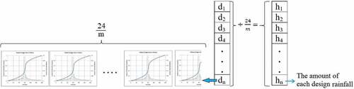
Since daily rainfall data are not sufficient for flood studies in urban areas, we introduce here a simple method for disaggregating daily rainfall time series to hourly data. It is quite obvious that, even with hourly data, the fast dynamics in the runoff process cannot be captured; but, given the size of the case study area, the temporal segregation is sufficient for the problem at hand. The methodology is based on the temporal distribution pattern of the precipitation for a specific region. Let the duration of typical rainfall in a region be m, the number of statistical years be z, and n = (z × 365) represent the total number of days in a precipitation time series. First, the amount of rainfall data in the daily time series is divided by 24/m. The resulting values for each single datum (h_n) are considered to represent the cumulative m-hour rainfall, there being a number 24/m of m-hour rainfalls within a day. If the remainder of 24/m is called b, then we will have 24/m of typical rainfall plus (b × m) hours of rainfall, giving 24/m + (b × m) typical storms of that region occurring on a particular day. Given the temporal rainfall distribution pattern for the study region, the amount of rainfall in each hour can be determined. The algorithm for the proposed disaggregation method is presented in Figure 2.

Figure 2. Proposed simple disaggregation method.

2.3 Rainfall–runoff modelling

The current study uses the storm-water management model of the US Environmental Protection Agency, SWMM version 5 – a widely used urban flood management model – as a tool to simulate hydraulic and hydrological processes in rainfall–runoff modelling of the urban drainage network. This software is a dynamic rainfall–runoff simulation model, which is used for single event or long-term (continuous) simulation of runoff (quantity and quality) in urban areas. The model simulates different processes in the drainage network and calculates flow discharge, flow depth, and water quality in each conduit during a simulation period and at the end (outfall) of the catchment (Rossman and Huber 2015). The SWMM model is normally used for simulating rainfall–runoff processes in urban areas; however, since urban drainage channels in Tehran are the continuation of rivers originating from upstream mountainous areas, the whole drainage network including natural and constructed channels was modelled through SWMM (considering the model capabilities).

The runoff transport system, with a total length of 67 km, mostly consists of open and covered channels with rectangular and horseshoe-shaped cross-sections, with widths of 1.4–30 m and heights of 1.4–6 m. Dynamic wave routing was considered as the flow routing method for simulation of runoff through the drainage system, which accounts for backwater effects and is capable of simulating mixed flows, reverse flows and rapidly varying flows. The infiltration process was modelled using the curve number (CN) method since such values were available from previous studies (Parsa and Moti’ee 2013) (Fig. 3) for each sub-basin. The curve number for each sub-basin has been calculated using hydrological soil groups (B and C) and the basin land-use maps in GIS environment. The soil-type map was available from Tehran Center of Earthquake (2000), based on which the hydrological soil groups are recognized.

Figure 3. Curve number values for the sub-basins of the study area (Parsa and Moti’ee 2013).

Manning’s coefficient (n) was estimated based on values presented by Mccuen (1974) for permeable and impermeable surfaces, while values of n for various channel materials were taken from ASCE (1982).

The study area, which contains three catchments: Darake, Farahzad and Hesarak, was divided into 23 sub-basins, of which three units are mostly considered as suburban areas and only their inflow to the urban areas is important. The boundary of each sub-catchment was determined based on the runoff flowing out to a channel or waterway through junctions using a current layout map of channels and a topographic map at the scale of 1:2000. Each sub-catchment width was calculated through dividing the area by the longest waterway in that specific sub-catchment. Also, surface storage values for permeable and impermeable surfaces were obtained from the SWMM user manual. Other required information for simulating the urban drainage network – such as channel dimensions and the elevation of the junctions – were obtained from information available from Mahab Ghods Consulting Engineering (MGCE).

Since the dimensions and characteristics of different parts of the channels were different, additional junctions were considered alongside each conduit to be able to delineate varying dimensions and conditions of the drainage network accurately; however, each sub-basin is only connected to the related junction of that district. Eventually, the modelled network included a total of 73 junctions plus an outfall node, and 73 links as the drainage conduits.

River streams were also modelled using SWMM considering the model capabilities in simulating various types of conduits/streams with different kinds of cross section. In this study, the non-urban areas were also simulated in SWMM since they include some impervious areas (such as urban districts) and because SWMM has the capability to model the rivers as a natural drainage conduit.

The design rainfall intensity was calculated using available IDF curves presented for Tehran and the equation offered by MGCE and Pöyry (MGCE and Pöyry 2011):

(1) $i=C_{\mathrm{A}\mathrm{l}\mathrm{t}.\mathrm{R}\mathrm{P}}{D}^{-0.645}$(1)

where i is rainfall intensity (mm/h) and D is rainfall duration (min; D ≤ 360 min), and $C_{\mathrm{A}\mathrm{l}\mathrm{t}.\mathrm{R}\mathrm{P}}$ is a coefficient that is dependent on design rainfall return period T (year) and mean ground elevation H (m a.s.l.):

(2) $C_{\mathrm{A}\mathrm{l}\mathrm{t}.\mathrm{R}\mathrm{P}}=108\left(0.0008H+0.2\right)\times \left(0.304\times \mathrm{l}\mathrm{n}\left(T\right)+0.78928\right)$(2)

Equation (2) depends on rainfall duration (min) and a coefficient dependent on ground level and rainfall return period. In addition, the temporal distribution of precipitation was according to what has been offered by MGCE. Since the ground elevation has a great difference between northern and southern parts of the studied watershed, two raingauges were applied for the upper and lower sub-basins. In Tehran’s northern areas, rainfall duration is mostly 6 or 7 h (Nazif 2010), so the duration of design rainfall was considered to be 6 h. In addition, a 10-min time step was applied in design rainfall time series as input to the model; and for long-term continuous input rainfall, the time intervals are daily, which is converted to hourly data through a simple method introduced in the following sections. The output runoff was extracted in 15-min time intervals. It should be noted that reduction in conduit capacity (due to sedimentation or blockage) for runoff transition is ignored in this study.

2.3.1 Calibration and sensitivity analysis

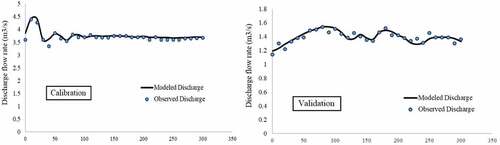
In order to determine which parameters have most effect on the model output (i.e. discharge from the basin), sensitivity analysis was performed. To do this, the one-at-a-time (OAT) method was employed (Saltelli and Annoni 2010). This is a simple method for sensitivity analysis which does not need high computational effort and, therefore, is widely used (Karamouz et al. 2016). In this technique, the model output is computed by varying one input factor at a time, while keeping the others unchanged. In this study, the model parameters were changed in 10% intervals within their permissible extent (presented in Table 2) to outline the effect to the flow rate at the catchment outfall. Calibration was conducted using the time series of discharge flow rate, depth and velocity, recorded every 10 min at the basin outlet by Moafi Rabari (2012), following a 17 mm storm on 27 December 2011. Validation was also performed through recorded data of a 12.5 mm rainfall event and consequent runoff at the basin outlet (Moafi Rabari 2012).

Table 2. Key model parameters involved for sensitivity analysis in this study, and their allowable extent for change (Li et al. 2014).

Parameter	Description	Range
n-Imperv	Manning’s n for impervious area	0.005–0.05
n-Perv	Manning’s n for pervious area	0.05–0.50
Dstore-Imperv	Depth of depression storage on impervious area (mm)	1.3–2.5
Dstore-Perv	Depth of depression storage on pervious area (mm)	2.5–7.6
Zero-Imperv	Percentage of impervious area with no depression storage (%)	50–80

The SWMM model was run for both continuous and single-event rainfall. First the design rainfall (a 5-year 6-hour rainfall) was simulated in order to get a general overview of UDS current performance in sustaining a rainfall typical for the catchment. A period of 5 years is the rainfall return period for which the UDSs are designed and are expected to be able to convey the produced runoff safely; and 6 hours is typical duration of design rainfall usually considered in the study area (Nazif 2010, MGCE and Pöyry 2011). Rainfall–runoff computations have been conducted for a continuous rainfall time series as the base line of future climatic computations.

2.4 Measuring UDS sustainability

2.4.1 Defining the type of disturbance

Urban drainage systems are exposed to different kinds of disturbance including climate change and rapid urban development. The former affects the UDS performance through changing precipitation regime, and the latter by reducing permeable areas. Both types of disturbance have the potential to cause pluvial flooding in urban areas. In the current study, extreme rainfall originating from climate change conditions is considered as the disturbance for UDS.

2.4.2 What is meant by UDS sustainability?

As an approach to urban drainage management, sustainability of UDS is defined as the ability of a disturbed system to resist and adapt to new conditions, as well as showing an acceptable level of performance and, ideally, improving the performance level at the end of the recovery process. Such a definition emphasizes the key indicators of post-disturbance sustainability including UDS robustness, reliability, resilience and adaptability to the new conditions of system. Robustness is about maintenance of system performance under disturbance and enduring the imposed changes without adapting (Husdal 2010). Thus, a system may be robust, yet not reliable. When a system is reliable, it means the performance is higher than an acceptable level. Sometimes, a system can be marked as “robust” even if the instant performance is not high enough. Here, we aim to determine how much resistance the system will show when subject to future rainfall-induced runoff. In such a definition, the number of system failures due to climate change may be satisfactory compared to the base line, but it is still non-reliable. By calculating adaptability, we are going to determine the degree to which the system shows better performance while subject to future changes, with or without using adaptive solutions.

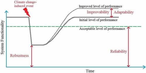
A system is, generally, considered resilient if it is able to survive and return to its normal or acceptable level of performance after the disturbance has been removed and the system has adapted to the new condition; however, ideally, the system may reach an improved functionality at the end of the recovery process (Rockefeller Foundation 2015, Maynard et al. 2017), referred to hereafter as “improvability”. Resilience can be defined through its various components, among which we focus on system improvability in performance after adapting to future climatic conditions. It is also noteworthy that, in the current study, we do not aim to investigate all sustainability components and indicators, but the goal is to examine the effectiveness of implementing BMPs on a larger scale for reducing urban flooding and measuring the degree of system efficiency through four types of index: reliability, robustness, improvability and adaptability (Fig. 4), three of which (i.e. robustness, improvability and adaptability) underlie the resilience characteristic of the system. Such indices relate the performance of the UDS in a changing climate to the amount of surcharge from the system and inundation problems that may occur due to insufficient capacity for conveying the storm-water runoff.

Figure 4. Schematic diagram of system behaviour following a climate change-induced disruptive event.

2.4.3 Performance assessment

The results of simulated runoff by SWMM were used to compute reliability, robustness, improvability and adaptability indices in order to assess the performance of urban drainage networks in the study area. Hashimoto et al. (1982) first formulated reliability for evaluating the possible performance of water resource systems. Following that, other researchers used the criterion after adapting it to the type of water resource or infrastructure under investigation (Kundzewicz and Kindler 1995, Fowler et al. 2003, Kjeldsen and Rosbjerg 2004, Jain and Bhunya 2008, Jain 2010, Ingol-Blanco and McKinney 2011, Asefa et al. 2014, Behzadian et al. 2014, Hoque et al. 2014, Xu et al. 2017). Reliability represents the likelihood of a system being in a satisfactory state.

In the current study, performance assessment of UDS was investigated through calculating different types of sustainability indices, including some robustness and reliability indicators adapted from the literature and some simple newly developed indices for system improvability and adaptability.

2.4.4 Hydraulic reliability

In general, the reliability can be expressed as the ratio of the number of satisfactory states to the total number of system activities. According to Kritskiy and Menkel (1952), three types of reliability can be discussed, each one describing the system performance from a different angle (Kundzewicz and Lasky 1995), namely, occurrence reliability, temporal reliability and volumetric reliability.

Occurrence reliability emphasizes the probability or the number of times a satisfactory state has occurred during a certain number of time steps. In the case of UDS, the hydraulic reliability index (HRI) can be defined as the ratio of the total number of time intervals in which a system is able to convey the runoff flow without surcharging to the total simulated time steps, i.e.:

(3) $\mathrm{H}\mathrm{R}{\mathrm{I}}_{\mathrm{o}}=\frac{1}{N}\sum _{t=1}^N{Z}_{\hspace{0.17em}}$(3)

with

(4) $Z_t=1\mathrm{\forall }{\mathrm{X}}_t\in S$(4)

(5) $Z_t=0\mathrm{\forall }{X}_t\in F$(5)

where $Z_t$ is the state of the drainage system in the time interval t, $X_t$ is the value of investigatory parameter in the time interval t, S is the satisfactory state, F is the failure state, and N is the total number of time intervals. A “satisfactory state” in such a simulation is defined as the state in which the system is able to convey the runoff flow without surcharging, here meaning runoff depth not to exceed the channel height. Accordingly, failure states are considered to be time intervals during which the flow exceeds the channel capacity (flow depth exceeds channel height) in the whole system.

Temporal reliability represents the amount of time the system remains in the satisfactory state divided by the total range of time considered, which can be expressed mathematically as:

(6) $\mathrm{H}\mathrm{R}{\mathrm{I}}_{\mathrm{T}}=1-\left(\frac{1}{T}\sum _{j=1}^M{T}_j\right)$(6)

where M is total number of system failures, i.e. surcharges, j is the count of number of failures, T_j is the duration for which the system remains in the failure mode j, and T is the duration of the operating period.

Volumetric reliability considers the ratio of water volume conveyed safely through the drainage system to the total runoff volume generated from rainfall, which is given by:

(7) $\mathrm{H}\mathrm{R}{\mathrm{I}}_{\mathrm{V}}=1-\left(\frac{1}{V}\sum _{j=1}^M{V}_j\right)$(7)

where M, again, is total number of system failures, j is the counter of number of failures, V_j is the water volume surcharged from the UDS in the failure mode j, and V is the total volume of storm-water runoff generated by the given rainfall.

2.4.5 System robustness

As pointed out earlier, system robustness is the ability to endure changes without adapting (Husdal 2010), and it indicates the level of system resistance to a disturbance so that the system continues moving in the same direction without degrading its performance. Therefore, in order to calculate system robustness, we should investigate which conduits in the drainage network are not surcharged when exposed to future climatic conditions, without considering adaptive strategies. In this sense, robustness can be calculated as:

(8) $\mathrm{R}\mathrm{o}\mathrm{b}\mathrm{u}\mathrm{s}\mathrm{t}\mathrm{n}\mathrm{e}\mathrm{s}\mathrm{s}=\frac{N_{\mathrm{c}\mathrm{n}\mathrm{s}}}{N}$(8)

where N_cns is the number of conduits in the system without surcharging in a changing climate, and N is the total number of conduits in the UDS.

2.4.6 Adaptability to climate change

In order to assess the ability of the system to perform acceptably in a changing climate, a new indicator is introduced, the climate change adaptability index (CCAI). The value of the CCAI for each node in the simulated network is defined as the probability (P) of the number of time steps in a study period when the simulated surcharged volume of storm water from the system in a future climate condition (R_f) does not exceed the simulated surcharged runoff volume in base-line climatic conditions (R_b):

(9) $\mathrm{C}\mathrm{C}\mathrm{A}\mathrm{I}=P\left(R_{\mathrm{f}}\le R_{\mathrm{b}}\right)=\frac{\mathrm{n}\mathrm{u}\mathrm{m}\mathrm{b}\mathrm{e}\mathrm{r}\mathrm{o}\mathrm{f}\mathrm{t}\mathrm{i}\mathrm{m}\mathrm{e}\mathrm{s}\mathrm{w}\mathrm{h}\mathrm{e}\mathrm{n}{R}_{\mathrm{f}}\le R_{\mathrm{b}}}{T}$(9)

where T is the total number of time steps in the simulated period.

The value of CCAI varies between 0 and 1, where 0 represents No Adaptation and 1 indicates Full Adaptability to climatic change. Other values of CCAI are interpreted in Table 3. In Figure 5, low and high adaptation areas are depicted in a pair-wise comparison of base-line and future surcharge from the UDS.

Table 3. Evaluation of the CCAI calculated values.

CCAI	Level of system adaptability to climate change
0 < CCAI ≤ 0.3	Very Low
0.3 < CCAI ≤ 0.5	Low
0.5 < CCAI ≤ 0.7	Medium
0.7 < CCAI ≤ 0.9	Good
0.9 < CCAI ≤ 1.0	High

Figure 5. Conceptual illustration of the climate change adaptability index, CCAI.

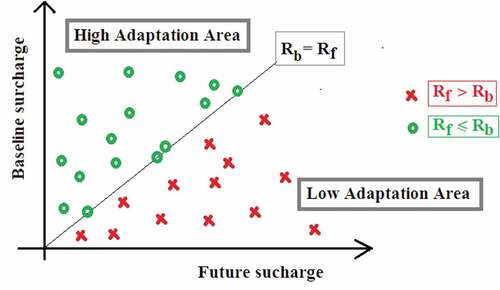
The CCAI evaluates the UDS adaptability using only one major parameter, i.e. runoff surcharge from the UDS, which is considered as flooding/inundation herein. Such a simple index, which does not require a vast range of parameters, can be helpful in gaining insight into the potential ability of the system to adjust itself to future climatic changes as well as evaluating the efficiency of the utilized adaptive measures in a changing climate. One can use it to know how adaptable the system is right now compared to past years/decades only if data regarding the runoff surcharges from the UDS are available; however, if CCAI is going to measure the level of adaptability to future climatic changes, predicting future climate conditions using climate model outputs alongside the rainfall–runoff modelling will be required.

2.4.7 Improvability of the system

Improvability can be defined as the degree to which system performance improves to a higher level after recovery from a disturbance, whether as a result of using adaptive strategies or without them. In the case of urban storm-water infrastructure, an improvement in performance (compared to the base line) normally happens after adaptation measures are used. In order to measure improvability of the system, the difference between hydraulic reliability indices in base-line and future conditions is obtained for each conduit and the average is calculated as the whole system improvability:

(10) $\mathrm{I}\mathrm{m}\mathrm{p}\mathrm{r}\mathrm{o}\mathrm{v}\mathrm{a}\mathrm{b}\mathrm{i}\mathrm{l}\mathrm{i}\mathrm{t}\mathrm{y}=\frac{{\sum }_{i=1}^{N_{\mathrm{s}\mathrm{b}}}(\mathrm{R}\mathrm{e}{\mathrm{l}}_{i\mathrm{f}}-\mathrm{R}\mathrm{e}{\mathrm{l}}_{i\mathrm{b}})}{N_{\mathrm{s}\mathrm{b}}}$(10)

in which Rel_ib and Rel_if are the reliability of the ith conduit in the UDS in base-line and future time periods, respectively, and N_sb is the number of surcharged conduits in the base time period for which Rel_if > Rel_ib.

2.5 Implementing BMPs in the catchment

Since part of the study area is located on the steep slopes of the northern part of Tehran, the basin has a short time of concentration; i.e. the time of concentration for all sub-basins of the study area is less than 1 h, which means the probability of flood occurrence is high. Therefore, enhancing appropriate types of BMPs could help to delay the peak time of urban floods (Karamouz et al. 2011). Field surveys and studies performed by different researchers have introduced certain types of BMPs for the north of Tehran, including the study area (Karamouz et al. 2011, Oraei Zare et al. 2012, Ahmadisharaf et al. 2015). According to such investigations, “bioretention basins” are among the best possible BMPs that can be applied in suburban areas of the region. A bioretention basin is an infiltration device used for both improving the quality and reducing the quantity of storm-water runoff (Dane County Water Resource Engineering 2007). They are vegetated areas with various underlying soil types (Stormwater Consulting Pty Ltd 2015). However, the study carried out by Tahmasebi Birgani et al. (2013) on an urban part of the nearby catchment indicated that porous pavement is the most suitable BMP considering technical, environmental and economical viewpoints. In addition, one of the most applicable BMPs proposed by some experts (Zohouri 2015) for the conditions of Tehran is porous pavement.

In the current study, bioretention ponds were considered for suburban areas that are non-residential and have the required space for such large BMPs (compared to urbanized areas), and porous pavement was applied to urban parts of the watershed. For the sake of simulating such a BMP in SWMM, storage depth was considered to be 150 mm and 0.9 was considered as vegetation volume fraction. In the soil layer, the thickness, soil porosity volume fraction and hydraulic conductivity were taken as 750 mm, 0.4 and 100 mm/h, respectively. For the gravel layer, which represents the actual storage space, the height, porosity and conductivity were input to the model with the values 200 mm, 40% and 350 mm/h, respectively (Tetra Tech, Inc. 2008). Porous pavement was assumed to be applied to half of the main streets in the whole catchment (Behroozi et al. 2015), i.e. a total of 32 000 m in length. Appropriate locations for applying the selected BMPs in the sub-basins were chosen based on available maps of the region.

Porous pavement (PP) is a paved pervious surface with less fine aggregates than conventional paving (California State University Sacramento 2016), and could be constructed in two main forms: pervious concrete and asphalt surfaces. According to the condition of the studied area, concrete PP is suggested here due to its significant advantages compared with asphalt PP for the studied region, including greater durability due to less susceptibility to ravelling or breakdown of the material, and reducing daytime temperatures and thus minimizing the urban heat island effect (Custom Concrete Contracting, Inc. 2016). This is considered to be a potential benefit of BMPs as an adaptive tool for facing climate change. Asphalt PPs have better performance in cold weather conditions; however, since in the studied region the winter is not too hard, concrete deterioration is not considered a major challenge (Wolf 2016). The installation cost for concrete PP is around 35% higher than asphalt porous pavement (Custom Concrete Contracting, Inc. 2016, Wolf 2016).

The given PP system consists of concrete pavers with permeable joint materials at the top, an open-graded bedding course underlain by an open-graded base and a sub-base reservoir consisting of washed, bank-run gravel (Stormwater Management Manual 2008), with a woven geotextile fabric located under the sub-base, underlain by uncompressed permeable sub-grade soil (Low Impact Development Center, Inc. 2012, Aztec Online 2018). To model the porous pavement in SWMM, some special parameters should be known or approximated rationally. In the current study, the PP surface slope was considered as 1% (Smith 2006), which is a smaller slope compared to the regional ground slope, in order to modify the high slope of the studied region. In addition, the values used for pavement thickness, surface storage depth, pavement void ratio and storage void ratio are 80 mm, 0, 0.2 and 0.4, respectively. The impervious surface fraction, which is the ratio of impervious paver material to total area for modular systems, was 0.82. The permeability value used was 0.75 mm/h for 20-year traffic (Smith 2006, Behroozi et al. 2015). Minimum hydraulic conductivity was assumed to be 500 mm/h (Montes and Haselbach 2006) and storage height was taken as 300 mm to be able to bear hydraulic load, according to Smith (2006) and Behroozi et al. (2015).

3 Study area

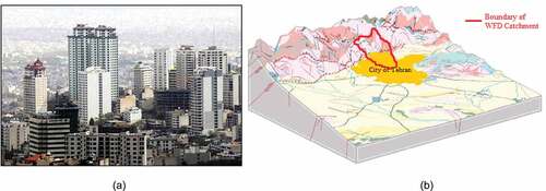
Rapid development of urban areas without considering the impacts on the water cycle has resulted in a wide range of challenges for water-related infrastructure in such cities. Tehran, the capital of Iran, is no exception. The Tehran West Flood Diversion (WFD) catchment was considered as the case study in this paper. The WFD covers an area of 142.63 km² and is located between 35°48′30″–35°52′49″N latitude and 51°19′13″–51°22′29″E longitude, including both urban and mountainous sub-basins. Three rivers, the Darakeh, Farahzad and Hesarak, transport the runoff from undeveloped sub-catchments into the urbanized parts of the watershed. In the urban parts, transferring the rainfall induced runoff is accomplished by several drainage channels, namely: Tappe Neyzar, Shahin and Shaghayegh, Morad Abad, Khoshke, Abdol Abad, Sa’adat Abad, Niyayesh and Behroud channels. All of these enter the WFD channel which discharges to the Kan River (Moafi Rabari 2012). Figure 6 shows the location of the studied area in the city of Tehran in Iran.

Figure 6. Situation of the studied watershed in Tehran, Iran.

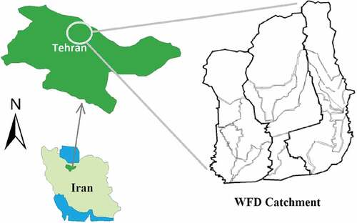
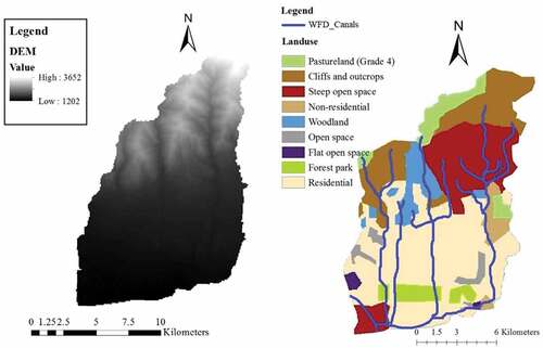
The catchment is mountainous in the northern parts and the difference in height of the catchment between northern and southern areas is up to 2400 m. The main land-use types in the catchment include residential (35%), steep open spaces (19%), and cliffs and outcrops (17%); however, in a few places, other types of land use such as pastures (8%), woodlands (7%), forest-parks (5%), open spaces (5%) and non-residential areas (4%) may be observed. In the mountainous upland areas, the land is mostly covered by rocky hills and steep lands, and – in some parts – grasslands. Figure 7 shows the land-use map and digital elevation model (DEM) of the watershed.

Figure 7. DEM and land-use map of the study catchment.

4 Results and discussion

4.1 Results of sensitivity analysis and model calibration

As expressed earlier, sensitivity analysis is required in order to detect those parameters that have the greatest influence on the results of the model. Here, five main parameters of SWMM: ground slope, characteristic width of each sub-basin, percentage of impervious surfaces (%Imperv), roughness coefficient for pervious areas (n-Perv) and roughness coefficient for impervious areas (n-Imperv), were examined to find the degree to which the peak discharge at the outlet is sensitive to each parameter. The results of the conducted sensitivity analysis suggest that two main parameters, namely %Imperv and n-Imperv, were the most sensitive of all the parameters in estimating peak discharges from the catchment (i.e. the model output for the peak discharge is most sensitive to the value of these two parameters), and therefore should be exactly calibrated.

Figure 8 presents the results of model calibration and validation considering discharge from the catchment by comparing root mean square error (RMSE), mean absolute error (MAE) and Nash-Sutcliffe efficiency (NSE) (Table 4). The first two measures evaluate the accuracy of the model results based on the differences between the observed and simulated values; the closer these error-based measures are to zero, the more accurate the model is in simulating the given variable. The RMSE is the standard deviation of prediction errors and estimates how concentrated the data points are around the regression line (Deb et al. 2018), while the MAE calculates the sum of absolute differences between the observed and simulated values, and measures the average magnitude of the errors in a set of simulations without considering their direction (Wu et al. 2015, Choudhury and Pandey 2018). The NSE is a normalized measure (–∞ to 1.0) that calculates the relative magnitude of the residual variance compared to the measured data variance (Nash and Sutcliffe 1970, Moriasi et al. 2007, Schaefli and Gupta 2007). A value of 1.0 for NSE represents a perfect match of observed and simulated data; values closer to 1.0 are representative of better performance of the model in simulating the given variables, and values less than 0.0 indicate unacceptable performance. As indicated in Table 4, the values of the NSE coefficient fall between 0.65 and 0.75, which is interpreted as “good” performance of the model (Moriasi et al. 2007).

Table 4. Results of model calibration and validation. RMSE: root mean square error; MAE: mean absolute error; NSE: Nash-Sutcliffe efficiency.

Given variable at the outlet	RMSE	MAE	NSE
Calibration
Depth	0.0130	0.0081	0.74
Velocity	0.0614	0.0455	0.68
Discharge	0.0855	0.0589	0.67
Validation
Depth	0.0156	0.0106	0.71
Velocity	0.0744	0.0606	0.66
Discharge	0.0417	0.0302	0.69

Figure 8. SWMM calibration and validation.

4.2 Inundation locations in existing drainage system

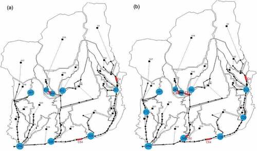
After calibration and performing rainfall–runoff modelling, it was found that, for a design rainfall with a return period of 5 years, eight nodes (J12, J29, J41, J49, J50, J51, J56 and J57) were flooded and three conduits (C4, C50 and C64) were surcharged. Considering the fact that the urban drainage network is usually designed to accommodate 2- to 5-year, or at most 10-year precipitation, it can be concluded that the existing drainage system of the study area should be rehabilitated, especially at the end of the studied watershed. The results of rainfall–runoff simulation for the base time period (1990–2006) indicate that four nodes (J50, J51, J56 and J57) and two conduits (C50 and C51) were inundated. Figure 9 illustrates the location of the flooded nodes and surcharged conduits for both event-based design rainfall and continuous base-line precipitation in the catchment. Table 5 presents the hydraulic reliability indices calculated for the surcharged conduit.

Table 5. Performance of surcharged conduits for the two rainfall scenarios. HRI: hydraulic reliability indicator; subscripts O, T and V refer to occurrence, temporal and volumetric, respectively.

Rainfall scenario	Surcharged conduit	HRIO	HRIT	HRIV
Design rainfall (single-event)	C4	90%	78%	73%
	C50	84%	70%	64%
	C64	86%	69%	67%
Continuous rainfall (1990–2006)	C4	89%	76%	69%
	C46	91%	74%	69%
	C50	81%	53%	42%
	C51	83%	64%	59%
	C64	85%	81%	75%

Figure 9. Inundation due to (a) 5-year 6-h rainfall, and (b) continuous rainfall in the base-line period.

4.3 Obtaining future climate change projections

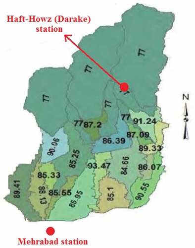
The only station located inside the WFD catchment that has an acceptable range of precipitation data recorded is Haft-Howz, which is actually a hydrometric station. In addition, Mehrabad synoptic station at the south of the catchment with enough recorded statistical data is a good choice for extracting precipitation data representing the catchment climate condition. According to the Intergovernmental Panel on Climate Change (IPCC), the base period of climatic studies should be considered as either 1961–1990 or 1971–2000 (IPCC-TGCIA 1999). In the current study, the 17-year period of 1990–2006 was considered as the base-line period, with respect to available precipitation data (there was a 17-year common statistical time period for both stations). Average rainfall for the catchment was calculated based on the height of either of these two stations and the average height of the whole watershed. Future projections for the catchment rainfall were investigated based on three 17-year periods: 2026–2042 as the near-term future, 2055–2077 as the mid-term future, and 2084–2100 for the distant future.

The MRI-CGCM3 model has been recognized as the appropriate AOGCM that provides the fewest errors in simulating rainfall in the studied catchment (Binesh et al. 2016). The MRI-CGCM3 model was developed by the Japanese Meteorological Research Institute (MRI) and has a resolution of 3.75° × 3.75° (Yukimoto et al. 2012). Future climate scenarios for three time horizons (2042, 2071 and 2100) were obtained using the MRI-CGCM3 model under the RCP4.5 emissions scenario. Table 6 presents the calculated changes of future predicted rainfall compared to the base-line observed data considering the long-term average values for each month.

Table 6. Variations in modelled future precipitation compared to the base-line observed rainfall (mm).

Month	2026–2042	2055–2071	2084–2100
Jan	69.05007	96.36114	67.41338
Feb	38.34926	44.5188	75.9411
Mar	28.97587	27.28938	34.48154
Apr	44.39144	16.04293	47.42728
May	11.29418	0.488659	−2.53088
Jun	6.007901	3.4554	1.251196
Jul	5.809621	−1.35789	−0.23586
Aug	0.480911	0.711598	0.664685
Sep	1.749327	1.845262	1.175328
Oct	16.28409	18.66907	12.5818
Nov	33.07126	37.04417	33.24056
Dec	23.17195	80.96605	80.72102

As can be seen from Table 6, the simulation results suggest that, in most months of the year, the values of precipitation increase significantly compared to the base-line period, and the largest change in rainfall amount is related to the months of January (for near-term and mid-term future) and December (for distant future).

4.4 Runoff simulation under climate change

Disaggregation of rainfall was performed for the studied area considering the fact that rainfall duration is almost 6 hours (Nazif 2010) and the rainfall temporal distribution pattern for the studied region was known (MGCE and Pöyry 2011), which resulted in having four 6-h rainfall events within a day. This means that, for the studied area, the 24-h rainfall can always be expressed as the sum of four 6-h rainfalls.

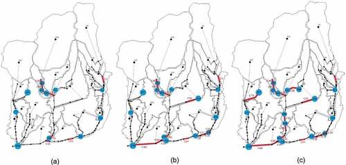
Disaggregated data on future rainfall for the three future time horizons (2042, 2071 and 2100) were used as input to the SWMM model. Figure 10 shows the inundation points and surcharged conduits for the studied future time periods. As can be seen in Figure 10, for the period 2026–2042, one more node (J52) was flooded and three more conduits (C34, C48, C49) were surcharged compared to inundation locations due to base-line rainfall. For the 2071 time horizon three other nodes (J26, J35 and J54) and seven other conduits (C25, C26, C27, C28, C52, C65 and C66) were additionally flooded and surcharged, respectively. Finally, for the period 2084–2100, three more nodes (J40, J44 and J45) and five other conduits (C25, C38, C42, C43 and C73) were added to the flooded and surcharged parts of the network.

Figure 10. Inundation locations and surcharged conduits for (a) 2026–2042, (b) 2055–2071 and (c) 2084–2100 time horizons in the WFD catchment.

4.5 Implementing BMPs

Given the flooded nodes and surcharged conduits calculated for normal and extreme rainfall events, it is understood that the existing drainage network is not reliable enough and should be improved using some kind of appropriate BMPs. In order to realize to what extent using BMPs will help to increase the sustainability of the drainage system, the chosen BMPs were applied alongside the UDS in two scenarios: (1) BMPs only in the urban basin, and (2) BMPs in both urban and upstream suburban areas. For comparison, there is also a “do nothing” scenario. Three hydraulic reliability indices (HRIs) were used for the assessment.

The tables in Appendix A indicate how installing BMP facilities alongside the drainage system may improve the performance of the drainage network in the study area. In Tables A1, A2 and A3, the number of failure modes, as well as HRIs for the surcharged links (conduits), can be compared for three given future time horizons. It should be mentioned that the number of failure modes is merely required for calculating “occurrence reliability”, since two other types of reliability (i.e. temporal and volumetric) are directly calculated from the results obtained by the SWMM model. The total number of time steps for rainfall–runoff modelling was 8029, and runoff simulation was done for 15-min intervals. In some cases, the number of failures for a conduit may be quite high, which results in lower occurrence reliability; however, small amounts of surcharging occur in each single failure mode, which results in high values of volumetric and, sometimes, temporal reliabilities. In contrast, there may be few failure modes and, thus, small values for the occurrence reliability, but with each failure mode including a high amount of surcharging from the system, resulting in high values of volumetric and temporal reliability.

As can be inferred from the tables in Appendix A, future changes of precipitation may affect the performance of the drainage system, since the number of surcharged conduits increases for all future time periods studied. The results also show that BMP implementation can enhance the reliability of the whole system and make up for the adverse impacts of possible future climate change on the drainage network’s efficiency. It is observed that the HRI would increase by up to 19 and 26% through BMP implementation in urban areas only and the whole catchment area, respectively. In addition, some conduits are no longer surcharged when using the BMPs. Such findings indicate the effectiveness of BMP usage, especially in upstream suburban areas of the catchment.

From Table A1 it is evident that, for the period 2026–2042, using BMPs in both urban and upstream non-urban areas causes the values of the HRIs reach to more than 70%. This threshold value reduces for the mid-term future and is more than 60%. However, for 2084–2100 period, HRI values are mainly above 50% after BMP usage in both urban and suburban parts of the catchment. Such results suggest that, in spite of significant efficiency of utilizing BMPs all over the catchment, there are still some conduits that may not perform reliably under future climatic conditions. While the number of such conduits is not considerable, there may be still a need to use additional measures for flood control in such spots.

System improvability is also calculated for different future time periods and presented in Appendix B (Table B1), which indicates how much enhancement in UDS performance has been made considering the surcharged conduits in the base line. It is clear from Table B1 that improvability of the system increases when using BMPs upstream of the urbanized area. Table B1 also shows that exposure to future climate change and use of adaptive strategies improves the performance of the system (compared to the base line) for all studied time periods; however, the improvability index (IMPRV) is greater for near future scenarios and decreases towards the distant future.

Table 7. UDS robustness under future scenarios.

	Future time period
	2026–2042	2055–2071	2084–2100
System robustness	90%	80%	74%

Table B1. System improvability in different future time periods before and after BMP installation. IMPRV: improvability index; subscripts O, T and V refer to occurrence, temporal and volumetric, respectively.

Rainfall scenario	Surcharged conduit	IMPRVO	IMPRVT	IMPRVV	System improvability
2026–2042
Before BMP	C4	2%	17%	25%	18%
	C46	_	5%	2%
	C50	_	20%	25%
	C51	17%	36%	41%
	C64	8%	-	-
After BMP	C4	11%	24%	31%	28%
	C46	_	9%	7%
	C50	3%	25%	30%
	C51	83%	64%	59%
	C64	12%	_	3%
2055–2071
Before BMP	C4	_	15%	21%	17%
	C46	_	_	_
	C50	_	15%	14%
	C51	_	22%	30%
	C64	3%	_	_
After BMP	C4	11%	24%	31%	20%
	C46	_	_	4%
	C50	_	19%	19%
	C51	_	28%	35%
	C64	7%	_	_
2084–2100
Before BMP	C4	_	9%	17%	12%
	C46	_	_	_
	C50	_	9%	8%
	C51	_	11%	20%
	C64	_	_	_
After BMP	C4	_	13%	21%	15%
	C46	_	_	_
	C50	_	13%	12%
	C51	_	17%	25%
	C64	5%	_	_

Table 7 presents the results of calculating the UDS robustness under future climatic conditions. The calculated robustness indices indicate an acceptable level of robustness for the whole system.

4.5.1 Adaptability to future climate change

4.5.1.1 CCAI validation

To utilize the proposed CCAI index for examining the UDS adaptability to future climatic changes, it should first be validated. However, there are some limitations. For instance, the developed index cannot be measured in the study area or along the drainage network in reality, so one cannot compare the results obtained by the proposed formula to real values. The CCAI is, in fact, a simple indicator representing the degree to which the drainage system has not been hurt by climate change impacts and how effective adaptive measure have been; this is while no BMP is currently installed in the study basin. Nevertheless, the validation was performed by calculating CCAI values for each sub-catchment for the period 1990–2000 as the base line and 2005–2015 as the future time period. The results were compared to the only inundation map available for the region from Tehran Municipality (2011) (Fig. 11) giving a semi-qualitative validation method due to the limitations mentioned.

Figure 11. Comparison of CCAI results with inundated locations for the period 2005–2015 (adapted from Tehran Municipality 2011).

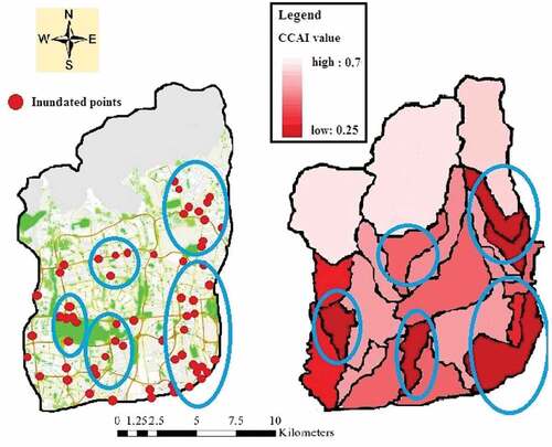
Since there was no observed data on storm-water runoff or number of surcharges from the UDS recorded for the catchment, rainfall–runoff modelling was performed for both 1990–2000 and 2005–2015, using the observed rainfall data (disaggregated into hourly data) as the input to the EPA SWMM. The rainfall–runoff simulation was accomplished and surcharge time series for the output nodes of the drainage network associated with each sub-catchment were obtained as a result. According to the calculated CCAI values, considering no BMP installation, the ability of the system to adapt to climatic changes was 0.7, at the very best, for the period 2005–2015, while there are at least four locations with very low adaptability (CCAI = 25). This result was obtained where the future and base-line periods considered for validation are quite close to each other, which means the adaptability of the system could be lower under a distant future scenario.

Although the CCAI value, being the ratio of 2005–2015 surcharge to a base-line surcharge from the UDS, and the hot-spots of inundation during the same period may not represent the same issue exactly, their coincidence with each other demonstrates the efficiency of the proposed index. This implies that the index is at least capable of predicting locations that might have significant inundation problems under the future scenario, and the results are not too far from reality.

4.5.1.2 Results of examining UDS adaptability in future periods

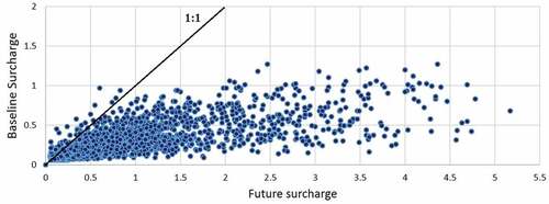
Figure 12 compares the calculated surcharges from the UDS for both the base line and the distant future at the basin outlet without BMP implementation in the catchment. It is observed that, for the majority of the 24 820 simulated time steps, the pairs are locate below the 1:1 line, which indicates that the number of surcharges from the drainage network in the distant future greatly exceeds those for the base time period. This represents a CCAI tending to zero and a “Low Adaptation” to future climatic changes, confirming the necessity of using adaptive strategies in the studied region.

Figure 12. Rate of change in surcharge from the UDS under the 2084–2100 scenario compared to 1990–2006 with no BMP implementation.

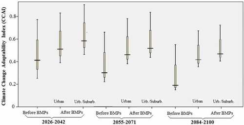
Figure 13 shows the extent of change in CCAI for different nodes of the system for future time periods. The SPSS (Statistical Package for the Social Sciences) was used to determine the range of CCAI changes in the whole system. As can be seen in Figure 13, the extent of flexibility against future climatic conditions is not high enough for different nodes of UDS. The adaptability of UDS for the No BMP scenario decreases from the near to the distant future, which indicates that the impacts of climate change are increasing as one moves towards the distant future. Similar to the results in Tables A1–A3 (Appendix A), using BMPs in urbanized areas causes the adaptability of the drainage system to increase for all time periods, while installing BMPs in both urban and upstream non-urban areas of the watershed (i.e. the whole watershed) is even more effective in enhancing the system performance and reducing the impacts of climate change for each given period. Instead, the range of changes in CCAI values gets smaller from the near future to the distant future. The difference between the adaptability index before and after BMP implementation is higher for 2084–2100 as compared to the earlier time periods, which suggests that using BMPs may be more effective in the distant future when the climate change impacts are greater than before. According to Table 3, it could be concluded that the system adaptability to climate change is Low to Medium, Low and Very Low for the near, mid-term and distant future, respectively. Although using BMPs enabled the adaptability level of the system to increase by one level, it is still at the Medium level at the very best, which means that, as suggested by the HRI values (Tables A1–A3), even using BMPs in the whole catchment, the adaptability of the system in a changing climate is not high enough. Therefore, using additional measures, including other types of BMP, should be examined in this study area.

Figure 13. Extent of CCAI in different nodes of the UDS before and after BMP implementation.

5 Lessons learnt for similar urbanized catchments

The specific conditions of the case studied here have the potential to provide some lessons for urban planners and decision makers in the sustainable management of semi-urbanized river basins with similar conditions. Some of the special characteristics of the study catchment include:

• a large population, rapid urban development, high building density, and high proportion of impermeable surfaces covering the urbanized sub-basin and low proportion of green spaces in the region (Fig. 14(a));

• the relatively high slope in the north (which is mostly non-urban) and much lower slope in the downstream urbanized region;

• the noticeable difference in altitude between northern and southern areas (Fig. 14(b));

• the low time of concentration and high potential of incorporating the storm-water runoff from the upland mountainous areas to the urbanized sub-basin in the downstream area;

• lack of BMP popularity even within urban areas; and

• a history of severe urban flooding and considerable inundation problems in rainy seasons.

Figure 14. (a) High density of buildings and lack of green space in Tehran and (b) difference in ground slope from north to south in the WFD catchment (source: YJC (Young Journalists Club) 2017, Tehran Municipality 2018).

The approach proposed in this study, which is based on a new definition for UDS sustainability, concentrated on system behaviour in the post-disturbance phase, and could be utilized for solving inundation problems in similar cases with a high potential of urban flooding. The introduced indices are simple enough to be used quickly and easily for gaining an insight into the UDS level of sustainability and to help urban managers take appropriate measures for preventing degradation of the performance of a drainage system.

6 Conclusions

Climate change introduces a challenge to UDSs, needing adaptive strategies to be considered to counteract such impacts. By introducing a framework for sustainability evaluation of an UDS, this paper provides an insight into the effectiveness of BMP usage on UDS sustainable performance by implementing the management strategies at two scales: the urban drainage basin level and considering the whole river basin. The assessments were made based on quantifying the performance of the UDS in a changing climate through calculating some indicators that represent the sustainability of the UDS. The main indicator was the reliability index, which was discussed from a hydraulic approach. Hydraulic reliability indices (HRIs) were used to compare the efficiency of implementing BMPs against flooding under different scenarios. Rainfall–runoff simulation under existing drainage conditions showed that the risk of flooding would significantly increase downstream of the studied watershed where the network receives runoff from different channels, and the situation would be worse under future climate scenarios. In addition, improvability of the system was examined to see how resilient it is to climatic changes. It was shown that the system is more resilient for the near future time period, but, even in the distant future, installing BMPs upstream of the urbanized area may enhance the improvability of the UDS. The calculated robustness indices are representative of an acceptable level of robustness for the whole system considering future long-term precipitation time series. However, if a single rainfall event is considered in the future, the system robustness may fail. It should be noted that the impact of extreme events on UDS robustness will be examined by the authors in another paper. The developed index for evaluating climate change adaptability (CCAI) is a simple tool, based on a few parameters, which can be useful for gaining insight into the ability of the system to adapt to new climatic conditions. Based on the results obtained for the CCAI, it could be said that the system indicates a lower level of adaptability in the distant future compared to earlier time periods; however, BMP implementation in the catchment was demonstrated to potentially enhance the level of adaptability to climatic changes, particularly if the upstream suburban areas are taken into account for BMP installation alongside the urbanized region.

The results of the study confirm the considerable effectiveness of applying BMPs in the urban sub-basin compared with the No BMP scenario, increasing the HRI by up to 19%. However, installing additional BMPs in upstream non-urban parts of the watershed had even more impact on the reduction in runoff volume, flooding occurrence and flood duration, making a 26% difference compared with the “do nothing” scenario. Such flow alleviation could be observed through increased values of reliability indices. In addition, the number of surcharged conduits and flooded nodes decreased when using BMPs upstream of the urban catchment. The performance of most failed conduits improved to above 50–90%, which is acceptable, but not satisfactory. The calculated adaptability index for the drainage network also indicated a significant risk of its being affected by adverse future hydro-climatic scenarios, even though two types of BMPs were installed in the whole catchment. Therefore, additional measures and other appropriate types of BMP approaches, such as enhancing grasslands in steep slopes of mountainous pre-urban areas, are recommended to gain more success in improving the drainage system performance.

It should be noted that, as mentioned as an assumption in the Introduction, blockage and sedimentation, which can result in reducing the capacity of the conduits, were not considered in this study, and this may affect the number of calculated inundation points and the value of performance indices in reality. Nevertheless, the results of this study can provide an overall insight and useful information for urban managers and water-sector decision makers considering adaptation strategies for improving urban storm-water drainage against future climate conditions in similar semi-urbanized catchments.

Disclosure statement

No potential conflict of interest was reported by the authors.

Notes

¹ https://www.dkrz.de/up/systems/wdcc.

Appendix A. Performance of surcharged conduits under different future scenarios with and without BMP usage

Table A1. Performance of surcharged conduits for the period 2026–2042 with and without BMP implementation. HRI: hydraulic reliability index; subscripts O, T and V refer to occurrence, temporal and volumetric, respectively.

Status	Surcharged conduit	No. of failures	HRIO	HRIT	HRIV
No BMPs	C4	1204	85%	88%	87%
BMPs, Only urban areas	C4	689	91%	93%	94%
BMPs, Both urban and sub-urban areas	C4	0	100%	100%	100%
No BMPs	C34	2235	78%	89%	84%
BMPs, Only urban areas	C34	1504	81%	96%	89%
BMPs, Both urban and sub-urban areas	C34	0	100%	100%	100%
No BMPs	C46	1351	83%	71%	66%
BMPs, Only urban areas	C46	1153	86%	79%	71%
BMPs, Both urban and sub-urban areas	C46	775	90%	83%	76%
No BMPs	C48	1756	78%	93%	88%
BMPs, Only urban areas	C48	0	100%	100%	100%
BMPs, Both urban and sub-urban areas	C48	0	100%	100%	100%
No BMPs	C49	2367	79%	89%	80%
BMPs, Only urban areas	C49	1799	87%	94%	91%
BMPs, Both urban and sub-urban areas	C49	0	100%	100%	100%
No BMPs	C50	2129	73%	64%	51%
BMPs, Only urban areas	C50	1653	79%	73%	67%
BMPs, Both urban and sub-urban areas	C50	1322	84%	78%	72%
No BMPs	C51	1678	79%	84%	87%
BMPs, Only urban areas	C51	0	100%	100%	100%
BMPs, Both urban and sub-urban areas	C51	0	100%	100%	100%
No BMPs	C64	1148	86%	67%	62%
BMPs, Only urban areas	C64	521	93%	75%	69%
BMPs, Both urban and sub-urban areas	C64	273	97%	81%	78%

Table A2. Performance of surcharged conduits for the period 2055–2071 with and without BMP implementation.

Status	Surcharged conduit	No. of failures	HRIO	HRIT	HRIV
No BMPs	C4	1598	80%	82%	84%
BMPs, Only urban areas	C4	1037	87%	91%	90%
BMPs, Both urban and sub-urban areas	C4	0	100%	100%	100%
No BMPs	C26	2753	66%	55%	48%
BMPs, Only urban areas	C26	2306	71%	68%	56%
BMPs, Both urban and sub-urban areas	C26	2003	75%	75%	61%
No BMPs	C27	2223	72%	89%	87%
BMPs, Only urban areas	C27	1267	84%	95%	91%
BMPs, Both urban and sub-urban areas	C27	0	100%	100%	100%
No BMPs	C28	1652	79%	92%	89%
BMPs, Only urban areas	C28	0	100%	100%	100%
BMPs, Both urban and sub-urban areas	C28	0	100%	100%	100%
No BMPs	C34	1728	78%	91%	84%
BMPs, Only urban areas	C34	1234	85%	97%	89%
BMPs, Both urban and sub-urban areas	C34	0	100%	100%	100%
No BMPs	C46	1589	80%	51%	56%
BMPs, Only urban areas	C46	1301	84%	64%	69%
BMPs, Both urban and sub-urban areas	C46	986	88%	69%	73%
No BMPs	C48	1645	79%	89%	84%
BMPs, Only urban areas	C48	990	88%	95%	89%
BMPs, Both urban and sub-urban areas	C48	0	100%	100%	100%
No BMPs	C49	2906	64%	84%	69%
BMPs, Only urban areas	C49	2533	68%	89%	76%
BMPs, Both urban and sub-urban areas	C49	2103	74%	93%	81%
No BMPs	C50	2529	69%	61%	47%
BMPs, Only urban areas	C50	2122	74%	68%	56%
BMPs, Both urban and sub-urban areas	C50	1704	79%	72%	61%
No BMPs	C51	2448	70%	75%	78%
BMPs, Only urban areas	C51	2007	75%	86%	89%
BMPs, Both urban and sub-urban areas	C51	1565	81%	92%	94%
No BMPs	C52	1143	86%	95%	91%
BMPs, Only urban areas	C52	0	100%	100%	100%
BMPs, Both urban and sub-urban areas	C52	0	100%	100%	100%
No BMPs	C64	1475	82%	61%	56%
BMPs, Only urban areas	C64	997	88%	66%	63%
BMPs, Both urban and sub-urban areas	C64	656	92%	70%	67%
No BMPs	C65	1197	85%	94%	90%
BMPs, Only urban areas	C65	0	100%	100%	100%
BMPs, Both urban and sub-urban areas	C65	0	100%	100%	100%
No BMPs	C66	3464	57%	68%	62%
BMPs, Only urban areas	C66	3032	62%	74%	69%
BMPs, Both urban and sub-urban areas	C66	2458	69%	81%	75%

Table A3. Performance of surcharged conduits for the period 2084–2100 with and without BMP implementation.

Status	Surcharged conduits	No. of failures	HRIO	HRIT	HRIV
No BMPs	C4	2067	74%	77%	79%
BMPs, Only urban areas	C4	1352	83%	85%	86%
BMPs, Both urban and sub-urban areas	C4	1005	87%	89%	90%
No BMPs	C25	2916	64%	43%	38%
BMPs, Only urban areas	C25	2354	71%	58%	49%
BMPs, Both urban and sub-urban areas	C25	1952	76%	64%	56%
No BMPs	C26	4056	49%	44%	39%
BMPs, Only urban areas	C26	3044	62%	59%	50%
BMPs, Both urban and sub-urban areas	C26	2628	67%	63%	55%
No BMPs	C27	3016	62%	74%	71%
BMPs, Only urban areas	C27	2486	69%	81%	77%
BMPs, Both urban and sub-urban areas	C27	2206	73%	85%	82%
No BMPs	C28	2044	75%	89%	86%
BMPs, Only urban areas	C28	0	100%	100%	100%
BMPs, Both urban and sub-urban areas	C28	0	100%	100%	100%
No BMPs	C34	3023	62%	49%	43%
BMPs, Only urban areas	C34	2522	69%	58%	49%
BMPs, Both urban and sub-urban areas	C34	2174	73%	62%	54%
No BMPs	C38	2020	75%	95%	91%
BMPs, Only urban areas	C38	0	100	100%	100%
BMPs, Both urban and sub-urban areas	C38	0	100%	100%	100%
No BMPs	C42	4016	50%	38%	35%
BMPs, Only urban areas	C42	3197	60%	49%	42%
BMPs, Both urban and sub-urban areas	C42	2875	64%	55%	46%
No BMPs	C43	3521	56%	51%	47%
BMPs, Only urban areas	C43	2396	70%	67%	58%
BMPs, Both urban and sub-urban areas	C43	2109	74%	72%	62%
No BMPs	C46	1956	76%	47%	52%
BMPs, Only urban areas	C46	1489	81%	60%	63%
BMPs, Both urban and sub-urban areas	C46	1186	85%	66%	67%
No BMPs	C48	2055	74%	84%	81%
BMPs, Only urban areas	C48	0	100%	100%	100%
BMPs, Both urban and sub-urban areas	C48	0	100%	100%	100%
No BMPs	C49	3045	62%	80%	64%
BMPs, Only urban areas	C49	2274	72%	85%	68%
BMPs, Both urban and sub-urban areas	C49	1787	78%	89%	73%
No BMPs	C50	3074	62%	56%	41%
BMPs, Only urban areas	C50	2026	75%	62%	50%
BMPs, Both urban and sub-urban areas	C50	1579	80%	66%	54%
No BMPs	C51	3096	61%	69%	71%
BMPs, Only urban areas	C51	2164	73%	75%	79%
BMPs, Both urban and sub-urban areas	C51	1799	78%	81%	84%
No BMPs	C52	1751	78%	92%	89%
BMPs, Only urban areas	C52	0	100%	100%	100%
BMPs, Both urban and sub-urban areas	C52	0	100%	100%	100%
No BMPs	C64	1950	76%	54%	51%
BMPs, Only urban areas	C64	1183	85%	63%	59%
BMPs, Both urban and sub-urban areas	C64	839	90%	67%	63%
No BMPs	C65	1633	80%	92%	87%
BMPs, Only urban areas	C65	0	100%	100%	100%
BMPs, Both urban and sub-urban areas	C65	0	100%	100%	100%
No BMPs	C66	5035	37%	46%	39%
BMPs, Only urban areas	C66	4036	49%	51%	47%
BMPs, Both urban and sub-urban areas	C66	3708	54%	56%	51%
No BMPs	C73	1523	81%	96%	92%
BMPs, Only urban areas	C73	0	100%	100%	100%
BMPs, Both urban and sub-urban areas	C73	0	100%	100%	100%

Appendix B. Urban drainage system improvability for different future time periods compared to the base line

References

- Ahmadisharaf, E., Tajrishy, M., and Alamdari, N., 2015. Integrating flood hazard into site selection of detention basins using spatial multi-criteria. Journal of Environmental Planning and Management, 59 (8), 1397–1417. doi:10.1080/09640568.2015.1077104
- Anandhi, A., et al., 2011. Examination of change factor methodologies for climate change impact assessment. Journal of Water Resources Research, 47 (3), W03501, 10. doi:10.1029/2010WR009104
- ASCE Task Committee on Relations Between Morphology of Small Streams and Sediment Yield of the Committee on Sedimentation of the Hydraulics Division, 1982. Relationships between morphology of small streams and sediment yields. Small Stream Morphology, 108 (HY11), 1328–1365.
- Asefa, T., et al., 2014. Performance evaluation of a water resources system under varying climatic conditions: reliability, resilience, vulnerability and beyond. Journal of Hydrology, 508, 53–65. doi:10.1016/j.jhydrol.2013.10.043
- Aztec Online, 2018. Best base for pavers permeable concrete paver design installation contractors [online]. Available from: http://www.fixsproject.com/best-base-for-pavers/best-base-for-pavers-permeable-concrete-paver-design-installation-contractors [Accessed 17 November 2018].
- Behroozi, A., Niksokhan, M.H., and Nazariha, M., 2015. Developing a simulation-optimization model for quantitative and qualitative control of urban run-off using best management practices. Journal of Flood Risk Management. doi:10.1111/jfr3.12210
- Behzadian, K., Kapelana, Z., and Morley, M.S., 2014. Resilience-based performance assessment of water-recycling schemes in urban water systems. 16th Conference on Water Distribution System Analysis, WDSA., Procedia Engineering, 89, 719–726.
- Berggren, K., Svensson, G., and Viklander, M., 2008. Urban drainage and climate change : a problematic approach ? In: Luleå University of Technology, Mistra-SWECIA (Mistra Swedish Research Programme on Climate, Impacts and Adaptation), Newsletter 1, Sweden.
- Binesh, N., Niksokhan, M.H., and Sarang, A., 2016. The effect of rainfall variability on Darakeh river flow rate during 1989–2012. Iranian Journal of Ecohydrology, 3 (3), 465–476(InPersian).
- Brown, J.L., et al., 2018. PaleoClim, high spatial resolution paleoclimate surfaces for global land areas. Journal of Scientific Data- Nature, 5, 180254. doi:10.1038/sdata.2018.254
- Cai, R., et al., 2011. Principal component analysis of crop yield response to climate change. Department of Agricultural and Applied Economics, University of Georgia, Faculty Series 103947.
- California State University Sacramento, 2016. California phase II LID sizing tool documentation manual, Prepared for: State Water Resources Control Board Proposition 84 Stormwater Grant, Agreement # 12-432-550. [Accessed 17 November 2018].
- Choudhury, S.D. and Pandey, S., 2018. Nth Absolute Root Mean Error, Cornel University Library, 12 Available from: https://arxiv.org/ftp/arxiv/papers/1810/1810.00421.pdf [Accessed 19 November 2018].
- Custom Concrete Contracting, Inc., 2016. Pervious concrete vs. porous asphalt, what is the difference? Available from: https://www.customconcrete.biz/2016/06/15/pervious-concrete-vs-porous-asphalt-what-is-the-difference [Accessed 16 November 2018].
- Da Silva, C.V.F., et al., 2018. Climate change impacts and flood control measures for highly developed urban watersheds. Journal of Water, 10 (829), 18.
- Dane County Water Resource Engineering, 2007. Dane county erosion control and stormwater management manual (Appendix I – bioretention basin), 4 Wisconsin, USA: Dane County Water Resource Engineering [Online] Available from: https://wred-lwrd.countyofdane.com/documents/ECSMManual/BioretentionBasin.pdf [Accessed 11 January 2018].
- Deb, B., et al., 2018. Travel time prediction using machine learning and weather impact on traffic conditions. BSc. Thesis. BRAC University, Bangladesh.
- Diaz-Nieto, J. and Wilby, R.L., 2005. A comparison of statistical down-scaling and climate change factor methods: impacts on low flows in the River Thames, United Kingdom. Journal of Climate Change, 69 (2–3), 245–268. doi:10.1007/s10584-005-1157-6
- Dudula, J. and Randhir, T.O., 2016. Modelling the influence of climate change on watershed systems: adaptation through targeted practices. Journal of Hydrology, 541 (Part B), 703–713. doi:10.1016/j.jhydrol.2016.07.020
- Fowler, H.J., Kilsby, C.G., and O’Connell, P.E., 2003. Modelling the impacts of climatic change and variability on the reliability, resilience, and vulnerability of a water resource system. Journal of Water Resources Research, 39 (8), 1222, 11.
- Gleick, P.H., 1986. Methods for evaluating the regional hydrologic impacts of global climatic changes. Journal of Hydrology, 88 (1– 2), 97–116. doi:10.1016/0022-1694(86)90199-X
- Goodarzi, E., et al., 2015. Evaluation of the change-factor and LARS-WG methods of downscaling for simulation of climatic variables in the future (case study: Herat Azam Watershed, Yazd -Iran). Ecopersia Journal, 3 (1), 833–846.
- Hailegeorgis, T.T. and Alfredsen, K.T., 2017. Analyses of extreme precipitation and runoff events including uncertainties and reliability in design and management of urban water infrastructure. Journal of Hydrology, 544, 290–305. doi:10.1016/j.jhydrol.2016.11.037
- Hashimoto, T., Stedinger, J.R., and Loucks, D.P., 1982. Reliability, resiliency, and vulnerability criteria for water resource system performance evaluation. Water Resources Research, 18 (1), 14–20. doi:10.1029/WR018i001p00014
- Hoque, Y.M., Hantush, M.M., and Govindaraju, R.S., 2014. On the scaling behaviour of reliability–resilience–vulnerability indices in agricultural watersheds. Journal of Ecological Indicators, 40, 136–146. doi:10.1016/j.ecolind.2014.01.017
- Hrdalo, I., Tomić, D., and Pereković, P., 2015. Implementation of green infrastructure principles in dubrovnik, croatia to minimize climate change problems. Journal of Urbani Izziv (I.E. Urban Challenge), 26 (special issue), 38–49.
- Husdal, J., 2010. A conceptual framework for risk and vulnerability in virtual enterprise networks: chapter 1. In S. Ponis, ed. Managing risk in virtual enterprise networks. ch 27, 1st ed. Business Science Reference.
- Ingol-Blanco, E. and McKinney, D., 2011. Analysis of scenarios to adapt to climate change impacts in the Rio Conchos Basin. In R.E Beighley II, ed. Proceedings of the World environmental and water resources congress 2011: bearing knowledge for sustainability, (Sponsored by the Environmental and Water Resources Institute of ASCE). California: Palm Springs, 1357–1364.
- IPCC, 2013. Climate change: action, trends and implications for business. Cambridge, UK: Cambridge University Press, Fifth assessment report of the Intergovernmental Panel on Climate Change (Working Group 1), 20 pp.
- IPCC-TGCIA (Intergovernmental Panel on Climate Change, Task Group on Scenarios for Climate Impact Assessment), 1999. Guidelines on the use of scenario data for climate impact and adaptation assessment. Version 1. Prepared by Carter, T.R., M. Hulme, and M. Lal, Intergovernmental Panel on Climate Change, Task Group on Scenarios for Climate Impact Assessment, p. 69.
- Jain, S.K., 2010. Investigating the behaviour of statistical indices for performance assessment of a reservoir. Journal of Hydrology, 391, 90–99. doi:10.1016/j.jhydrol.2010.07.009
- Jain, S.K. and Bhunya, P.K., 2008. Reliability, resilience and vulnerability of a multipurpose storage reservoir. Hydrological Sciences Journal, 53 (2), 434–447. doi:10.1623/hysj.53.2.434
- Kang, N., et al., 2016. Urban drainage system improvement for climate change adaptation. Journal of Water, 8 (7), 268. doi:10.3390/w8070268
- Karamouz, M., Hosseinpour, A., and Nazif, S., 2011. Improvement of urban drainage system performance under climate change impact: case study. Hydrological Engineering, 16 (5), 395–412. doi:10.1061/(ASCE)HE.1943-5584.0000317
- Karamouz, M., Zeynolabedin, A., and Olyaei, M.A., 2016. Regional drought resiliency and vulnerability. Journal of Hydrologic Engineering, 21 (11), 05016028. doi:10.1061/(ASCE)HE.1943-5584.0001423
- Kjeldsen, T.R. and Rosbjerg, D., 2004. Choice of reliability, resilience and vulnerability estimators for risk assessments of water resources. Hydrological Sciences Journal, 49 (5), 755–767. doi:10.1623/hysj.49.5.755.55136
- Kritskiy, S.N. and Menkel, M.F., 1952. Water management computations, GIMIZ, Leningrad (in Russian).
- Kundzewicz, Z.W. and Kindler, J., 1995. Multiple criteria for evaluation of reliability aspects of water resources systems. In: S.P. Simonovic, Z.W. Kundzewicz, D. Rosbjerg, and K. Takeuchi, eds. Modelling and management of sustainable basin-scale water resources systems. Wallingford, UK: International Association of Hydrological Sciences, IAHS Publication no. 231, 217–224.
- Kundzewicz, Z.W. and Lasky, A., 1995. Reliability-related criteria in water supply system studies. In: Z.W. Kundzewicz, ed. New uncertainty concepts in hydrology and water resources. Cambridge, England: Cambridge University Press, International Hydrology Series, 299–305.
- Li, C., et al., 2014. Sensitivity analysis for urban drainage modelling using mutual information. Journal of Entropy, 16 (11), 5738–5752. doi:10.3390/e16115738
- Low Impact Development Center, Inc., 2012. Permeable pavements [online] Available from: https://slideplayer.com/slide/3868839 [Accessed 17 November 2018].
- Maynard, T., et al., 2017. Future cities: building infrastructure resilience: city infrastructure resilience – designing the future. Lloyd’s project team, ARUP, Emerging Risk Report 2017, Society and Security.
- Mccuen, R.H., 1974. A regional approach to urban stormwater detention. Geophysical Research Letters, 1 (7), 1–2. doi:10.1029/GL001i007p00321
- Meinshausen, M., et al., 2010. The RCP greenhouse gas concentrations and their extensions from 1765 to 2300. Climate Change, 109, 213–241. doi:10.1007/s10584-011-0156-z
- MGCE and Pöyry, 2011. Tehran stormwater management master plan. Tehran, Iran: Mahab Ghodss Consulting Engineering Company (MGCE).
- Moafi Rabari, A., 2012. Optimal design of WFD (West Flood-Diversion) dimensions based on upland catchment’ characteristics. Msc. Thesis, University of Tehran.
- Montes, F. and Haselbach, L., 2006. Measuring hydraulic conductivity in pervious 20 concrete. Environmental Engineering Science, 23 (6), 960–969. doi:10.1089/ees.2006.23.960
- Moriasi, D.N., et al., 2007. Model evaluation guidelines for systematic quantification of accuracy in watershed simulations. Transactions of the ASABE (American Society of Agricultural and Biological Engineers), 50 (3), 885−900.
- Nash, J.E. and Sutcliffe, J.V., 1970. River flow forecasting through conceptual models: part 1. A discussion of principles. Journal of Hydrology, 10 (3), 282–290. doi:10.1016/0022-1694(70)90255-6
- Nazif, S., 2010. Developing an algorithm for climate change assessment on urban water cycle. Tehran, Iran: University of Tehran.
- Nie, L., et al., 2009. Impacts of climate change on urban drainage systems – a case study in Fredrikstad, Norway. Urban Water Journal, 6 (4), 323–332. doi:10.1080/15730620802600924
- Oraei Zare, S., Saghafian, B., and Shamsai, A., 2012. Multi-objective optimization for combined quality–quantity urban runoff control. Journal of Hydrology and Earth System Sciences, 16, 4531–4542. doi:10.5194/hess-16-4531-2012
- Parsa, V. and Moti’ee, H., 2013. Modelling urban floods using Storm-Cad. In: The 5th Conf. on Iran Water Resources Management. Tehran, Iran.
- Randall, D.A., et al., 2007. Climate models and their evaluation. In: Climate change 2007: the physical science basis. contribution of working group I to the fourth assessment report of the intergovernmental panel on climate change, 591–662. doi:10.1016/j.cub.2007.06.045
- Rao, Y.R.S. and Ramana, R.V., 2015. Stormwater Flood Modelling in Urban Areas. International Journal of Research in Engineering and Technology, 4 (11), 2319–2322.
- Rockefeller Foundation, 2015. City resilience and the city resilience framework [online]. Rockefeller Foundation, Available from: http://b.3cdn.net/rockefeller/b794a68196d5979dc2_f0m6i6owi.pdf [Accessed 6 December 2015].
- Rossman, L. and Huber, W., 2015. Stormwater management model reference manual volume I. Hydrology. Washington, DC: US EPA Office of Research and Development, US EPA Office of Research and Development.
- Saltelli, A. and Annoni, P., 2010. How to avoid a perfunctory sensitivity analysis. Journal of Environmental Modelling & Software, 25 (12), 1508–1517. doi:10.1016/j.envsoft.2010.04.012
- Sarr, M.A., et al., 2015. Comparison of downscaling methods for mean and extreme precipitation in Senegal. Journal of Hydrology: Regional Studies, 4 (Part B), 369–385.
- Schaefli, B. and Gupta, H.V., 2007. Do Nash values have value? Hydrological Processes, 21, 2075–2080. doi:10.1002/(ISSN)1099-1085
- Semadeni Davies, A., et al., 2008. The impact of climate change and urbanization on drainage in Helsingborg, Sweden: suburban stormwater. Journal of Hydrology, 350 (1–2), 114–125. doi:10.1016/j.jhydrol.2007.11.006
- Short, D., 2014. Regional climate change impact index. A case study: coastal British Columbia and Bangladesh. In: Viu Create: Celebration of research excellence and knowledge transfer event. Canada: Vancouver Island University.
- Smith, D.R., 2006. Permeable interlocking concrete pavements: selection, design, construction, maintenance. 3rd ed. Washington, DC: ICPI (Interlocking Concrete Pavement Institute).
- Stormwater Consulting Pty Ltd, 2015. Bio-retention basin, Online. Available from: http://www.stormwaterconsulting.com.au/quality.html [Accessed 11 January 2018].
- Stormwater Management Manual, 2008. Technical guidance, Knox County, TN. In: Chapter 4: porous Pavement. Lewis Publisher, Vol. 2, 189–200. Available form: https://knoxcounty.org/stormwater/manual/Volume%202/Volume2Combined.pdf [Accessed 25 August 2018].
- Tachiiri, K., et al., 2013. Allowable carbon emissions for medium-to-high mitigation scenarios. Tellus B: Chemical and Physical Meteorology, 65 (1), 24. Taylor & Francis group. doi:10.3402/tellusb.v65i0.20586
- Tahmasebi Birgani, Y., Yazdandoost, F., and Moghadam, M., 2013. Role of resilience in sustainable urban stormwater management. Journal of Hydraulic Structures, 1 (1), 42–50. Shahid Chamran University.
- Tajrishy, M., 2012. Introduction to modern techniques of stormwater management. In: Workshop on “Novel methods for collecting and management of urban stormwater runoff. Tehran, Iran: Tehran center for urban studies and planning.
- Tang, Q. and Oki, T., 2016. The terrestrial water cycle: natural and human-induced changes. In: Q. Tang and T. Oki, eds. (Geophysical Monograph 221, First Edit). American Geophysical Union, John Wiley & Sons, Inc., 252. doi:10.1002/9781118971772
- Tehran Center of Earthquake, 2000. Main report of study on seismic micro zoning of the greater Tehran area in the Islamic Republic of Iran, JICA.
- Tehran Municipality, 2011. Inundation map for Tehran streets, prepared by: communication and information technology agency. Available from: http://sdi.tehran.ir [Accessed 28 November 2018].
- Tehran Municipality, 2018. Geomorphology of Tehran region. Available from: http://atlas.tehran.ir/Default.aspx?tabid=167 [Accessed 24 November 2018].
- Tetra Tech ARD, 2014. A review of daownscaling methods for climate change projections. In: S. Trzaska and E. Schnarr, eds. African and Latin American resilience to climate change project. USA: US Agency for International Development (USAID), 65.
- Tetra Tech, Inc., 2008. Stormwater best management practices (BMP) performance analysis. Boston, MA: United States Environmental Protection Agency, 232.
- Thomson, A.M., et al., 2011. RCP4.5: a pathway for stabilization of radiative forcing by 2100. Climatic Change, 109, 77–94. doi:10.1007/s10584-011-0151-4
- Wang, L., et al., 2012. The East Asian winter monsoon over the last 15,000 years: its links to high-latitudes and tropical climate systems and complex correlation to the summer monsoon. Quaternary Science Reviews, 32, 131–142.
- Wilby, R. L., and Harris, I., 2006. A framework for assessing uncertainties in climate change impacts: low-flow scenarios for the river thames, UK, Journal of Water Resources Research, 42(2), 1–10. doi: 10.1029/2005WR004065
- Wolf, S., 2016. Asphalt pavement vs. concrete – which one should you choose? Available from: https://www.wolfpaving.com/blog/bid/85737/asphalt-pavement-vs-concrete-which-one-should-you-choose [Accessed 16 November 2018].
- Wu, H., et al., 2015. Personalized QoS prediction of cloud services via learning neighborhood-based model. In: 11th International Conference on Collaborative Computing: Networking, Applications, and Worksharing. Wuhan, China.
- Xu, B., et al., 2017. Optimal hedging rules for water supply reservoir operations under forecast uncertainty and conditional value-at-risk criterion. Journal of Water, 9 (8), 568, 17.
- YJC. (Young Journalists Club), 2017. How is the cost of water, electricity, gas and telephone shared between apartments? Available from: https://www.yjc.ir, [Accessed 24 November 2018].
- Yukimoto, S., et al., 2012. A new global climate model of the meteorological research institute: MRI-CGCM3-model description and basic performance. Journal of the Meteorological Society of Japan, 90, 23–64. doi:10.2151/jmsj.2012-A02
- Zhou, Q., Leng, G., and Huang, M., 2018. Impacts of future climate change on urban flood volumes in Hohhot in northern China: benefits of climate change mitigation and adaptations. Journal of Hydrology and Earth System Sciences, 22, 305–316. doi:10.5194/hess-22-305-2018
- Zohouri, S., 2015. The process of industrial installation of concrete pavements and related machinery performance. In: 2nd conference and exhibition of urban civil for city of Tehran. Tehran, Iran: Tehran Research Institute of Petroleum Industry (NIOC-RIPI).