Precipitation as a proxy for climate variables: application for hydrological modelling

ABSTRACT

It has been proposed that linear regression curves can be used to estimate monthly climate variables from observed precipitation. This approach was explored by applying the MGB hydrological model to the Paraná Basin (Brazil). Linear regressions were obtained for 54 climate gauges, and most of them showed at least six months of significant correlation between monthly climate variables (sunlight hours and relative humidity) and precipitation. The regression equations were applied to 5201 raingauges to estimate monthly climate variables and evapotranspiration, and the results were compared with a scenario using long-term climate averages only. The main differences occurred in wetter periods, where negative correlations between monthly precipitation and evapotranspiration were obtained when using precipitation as a proxy. Long-term changes in the hydrological regime were assessed and showed that the effect of precipitation on relative humidity and sunlight hours seems to have a minor effect on the alterations observed in river discharge in the Paraná Basin.

KEYWORDS:

• actual evapotranspiration
• precipitation as proxy
• climate data
• hydrological modelling
• Paraná River Basin

Editor R. Woods; Associate editor H. Kreibich

1 Introduction

Long-term climate variability may severely affect large river basins, altering hydrological and energy processes such as evapotranspiration in a complex way (Rasmusson et al. 1993). For instance, changes in precipitation relate directly to alterations in evapotranspiration. Considering that the main variable that explains potential evapotranspiration is incident radiation (Collischonn and Collischonn 2016), it follows that rainy periods tend to increase cloud cover, decreasing potential evapotranspiration. However, when it comes to actual evapotranspiration, a more complex situation is present – it depends also on soil water availability for plants and its influence on stomata opening, so that water can be released from soil to atmosphere (Bonan 2008, Zhang et al. 2008). As a result, basins may differ from energy-limited, where evapotranspiration occurs at near potential rates and the process is only halted by radiation availability, to water-limited ones, where dry periods may decrease evapotranspiration due to lack of water in the soil (Budyko 1958, Beven 1979, Bonan 2008). These different processes may act together in different regions of a large basin, leading to different responses in discharge generation during the hydrological year.

Estimating actual evapotranspiration at the basin or sub-basin scale is a challenging task, especially at monthly or daily time scales where simple water balance approaches are no longer applicable (i.e. E = P − Q), and information on basin water storage may be required (Zhang et al. 2008). Observational methods at local scale include resource-consuming lysimeters, leaf water loss measurements, Bowen ratio-based and eddy covariance techniques, which have limitations in terms of extrapolation for the basin scale. For this scale, hydrological studies usually employ remote sensing techniques or hydrological models, which in turn may be more conceptually (e.g. rainfall–runoff models) or empirically based (e.g. Budyko framework). In rainfall–runoff models, computation of evapotranspiration typically relies on observed data of climate variables at meteorological stations, which are then converted to evapotranspiration using resistance-based equations such as the Penman-Monteith method (P-M; Penman, 1960, Monteith 1965). Other approaches are still used as well, such as those based on water budget (Guitjens 1982), mass transfer (Harbeck 1962), radiation (Priestley and Taylor 1972), and temperature (Thornthwaite 1948, Blaney and Criddle 1950). However, the P-M method is recommended by the FAO (Food Agricultural Organization) as the sole method to calculate reference evapotranspiration wherever the required input data are available (Allen et al. 1998, Droogers and Allen 2002), and is today ubiquitous in hydrological models.

Especially in developing countries, data availability for evapotranspiration calculation using the P-M method is very limited (Gong et al. 2006, Wang et al. 2011, Corbari et al. 2014, Jury 2017), since it is necessary to monitor several climate variables for its calculation (e.g. air temperature, wind speed, relative humidity and shortwave radiation data). This lack of information has prompted several studies to understand the sensitivity of the P-M method to its input variables (Oudin et al. 2010, Li et al. 2016), and to obtain evapotranspiration from other sources such as combined model–remote sensing methods (Seevers and Ottmann 1994, Bastiaanssen et al. 1998, Su et al. 2005, Moiwo et al. 2011, González-Dugo et al., 2013, Ruhoff et al. 2013, Corbari et al. 2014, Seiller and Anctil 2015, Jung et al. 2016). Oudin et al. (2010) performed a sensitivity analysis of the P-M equation to different time availability of climate data for estimation of potential evapotranspiration, and concluded that using average climate data had little effect on estimating monthly and annual potential evapotranspiration, when compared to daily data based estimates. Recent studies developing new methods for evapotranspiration estimation at basin scale include the works of Gong et al. (2006), who studied the relative importance of climatic variables to the variation of P-M calculated evapotranspiration, and the work of Jury (2017) who addressed the use of satellite-model proxies for hydro-meteorological variables.

Alternatively, it is very common to rely on statistical methods for the correction or estimation of unknown variables (Wilby et al. 2000, Wood et al. 2004). With this insight, Collischonn and Tucci (2014) and Collischonn and Collischonn (2016) have used climate data from the Brazilian National Institute of Meteorology (INMET) to show the potentiality of using precipitation as an estimator (or a proxy) for other climate variables such as relative humidity, sunlight (or sunshine) hours and potential evapotranspiration. It should be possible with this approach to estimate these climate variables with a better temporal resolution than is usually available, since precipitation gauges are more frequent than full meteorological stations.

A statistical approach can then be very useful for hydrological modelling of ungauged basins, as in the context of prediction in ungauged basins (PUB; Hrachowitz et al. 2013), where climate data availability for earlier periods is generally low. For example, Collischonn and Collischonn (2016) mention that the Brazilian integrated hydropower network design and operation is based on river inflows during a dry sequence of years in the 1950s. Indeed, many large scale hydrological model applications today tend to use long-term averages (i.e. climate normals) for simulating discharges (e.g. Paiva et al. 2013, Pontes et al. 2017), given difficulties in obtaining or estimating observed climate data at daily or hourly resolution. The extent to which adopting long-term averages affects model discharge estimates is also poorly known, although errors in discharge estimation by not using daily climate data may be overcome by model overparameterization (see Beven 2006 for a discussion on parameter equifinality).

In this context, this work can be considered an extension of the study by Collischonn and Collischonn (2016), addressing the dynamics of actual evapotranspiration in a large scale basin. We use precipitation as a proxy of climate variables for estimating their monthly variation, allowing a more coherent comprehension of past hydrological alterations through hydrological modelling. The scientific questions of this research are: (1) Is there added value in the use of precipitation as a proxy of climate variables for hydrological models and estimation of actual evapotranspiration? (2) Once there is added value, is it possible to understand long-term changes in evapotranspiration rates better by adopting precipitation as proxy approach?

To address the proposed questions, in this study the MGB model (Collischonn et al. 2007, Pontes et al. 2017) is applied to the Upper Paraná River Basin in Brazil, forced with precipitation and climate data from the INMET database, and model results using precipitation as a proxy of climate variables are compared with runs using long-term climate averages. The model is then used to investigate changes in hydrological regime that have occurred in the basin during the past century, where a significant increasing trend has been observed in discharge since the 1970s (García and Vargas 1998). The possibility of using precipitation as a proxy of climate variables is especially useful in this case for extending climate data series estimates in order to better comprehend such changes.

2 Study area

The Paraná River Basin is an important region in South America, with more than 50% of the hydro-electric energy generation of Brazil (EPE, 2015) and major South American economic centres located within it, such as the cities of São Paulo and Brasília (Federal Capital). In this study, the basin was considered up to the downstream confluence between the Paraná and Iguaçu rivers, near the Itaipu Dam (~900 000 km²). The basin accounts for the second largest annual streamflow in the continent, after the Amazon River.

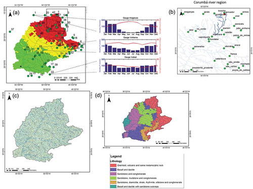
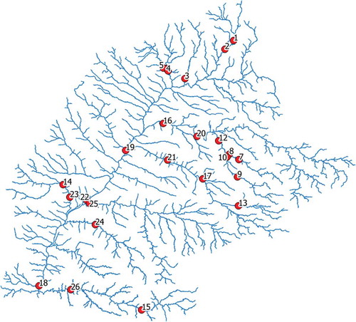
Due to its large spatial scale, the basin presents expressive climate variability. The northeast region has a warm, strongly seasonal climate, while the southwestern part features a more temperate climate, with evenly distributed precipitation over the year. Figure 1(a) shows the seasonality index for different regions, based on the methodology of Walsh and Lawler (1981), which relies on observed precipitation data. The 54 climate gauges from INMET used in this study are also presented. There is a large lack of data in the west of the basin, where the Ivinhema gauge (gauge 28) is the only one available. Finally, Figure 1(a) shows monthly precipitation and sunlight hours for three gauges, differing in terms of seasonality. The northern climate is typically more seasonal, with more sunlight hours during winter than the southern area, where precipitation is more evenly distributed throughout the year. According to Alvares et al. (2013), the Köppen climate classification for the basin is Aw (tropical with dry winter) in the north, Cwa (humid subtropical with dry winter and hot summer) and Cwb (humid subtropical with dry winter and temperate summer) in the northeast, Cfa (humid subtropical with oceanic climate without dry season and with hot summer) in the central-south region and Cfb (humid subtropical with oceanic climate without dry season and with temperate summer) in the south.

Figure 1. (a) Paraná River Basin, climate gauges and seasonality index along the basin. The two black squares indicate the Itaipu Dam (in the south) and the city of Brasília (in the north, above gauge no. 7), used in the analysis of Sections 4.2 and 4.3; (b) detail of the Corumbá River Basin (dark blue drainage), used for the analysis in Section 4.5, showing Roncador gauge (red dot), used because of the full availability of daily relative air humidity and hours of sunlight data; (c) the 1424 unit-catchments used for model calculation; and (d) lithological regions used for model calibration

3 Methods

3.1 MGB model

The MGB model is a semi-distributed, rainfall–runoff hydrological model developed to simulate large-scale basins (Collischonn et al. 2007, Pontes et al. 2017). The model has been successfully applied for a number of large basins in South America (Paiva et al. 2013, Fan et al. 2014).

In the MGB model, the basin is divided into unit-catchments (Fig. 1(c)), where vertical soil water balance is computed considering surface, subsurface and groundwater flow generation and interception and evapotranspiration processes. Water is then routed through the unit-catchment in linear reservoirs to the river drainage network, where a flood wave routing method is employed (Muskingum-Cunge or Local Inertial module). Model parameter datasets are given for hydrological response units (HRUs) inside each unit-catchment, which are defined as having homogenous land use and soil type areas. A complete description of the model is given by Pontes et al. (2017).

In the current application, one parameter dataset is provided for each lithological region in the basin, so that it considers the geological controls on rainfall–runoff processes. Traditional applications of the MGB model used sub-basins upstream of control discharge gauges to calibrate the model, but in this study we adopted a more physically-based calibration, based on a classification of main lithological areas within the basin (Fig. 1(d)). Within each lithological area, the model was calibrated for different HRUs defined from a map of HRUs for South America¹ (Fan et al. 2015).

Evapotranspiration is calculated with the Penman-Monteith formula (Equation (1)(1) $\mathrm{E}\mathrm{T}=\frac{\mathrm{\Delta }\left(R_n-G\right)+{\rho }_a{C}_p\left(e_s-e_a\right)/r_a}{\mathrm{\Delta }+\gamma \left(1+r_s/r_a\right)}\times \frac{1}{\lambda {\rho }_w}$(1) ), which depends on relative air humidity, atmospheric pressure, air temperature, sunlight hours (for radiation calculation) and wind speed data from the nearest climate gauge station (see Table 1 for data availability for each analysed gauge for these variables). To address the dependence of vegetation evapotranspiration on soil moisture availability, it is assumed that surface resistance increases linearly with soil moisture constraints after a threshold value is reached during dry periods (half of soil water maximum storage parameter) (Collischonn et al. 2007):

(1) $\mathrm{E}\mathrm{T}=\frac{\mathrm{\Delta }\left(R_n-G\right)+{\rho }_a{C}_p\left(e_s-e_a\right)/r_a}{\mathrm{\Delta }+\gamma \left(1+r_s/r_a\right)}\times \frac{1}{\lambda {\rho }_w}$(1)

Table 1. Daily data availability (percentage of total period) of sunlight hours (SH), relative humidity (RH), atmospheric pressure (AP), wind speed (WS) and average surface air temperature (ST) for each of the 54 INMET gauges. The starting date (dd/mm/yyyy) of data availability for each gauge is also given; the ending date of 31/12/2011 is the same for all gauges

ID	Gauge name	Starting date	SH	RH	AP	WS	ST	Daily precipitation
1	Aragarças	01/05/1970	80	92	92	92	84	91
2	Araxá	01/04/1963	77	80	82	82	76	81
3	Arinos	01/06/1976	71	88	89	89	79	87
4	Avelar	01/01/1985	88	71	95	95	94	71
5	Bambuí	01/01/1961	70	70	77	77	69	75
6	Barbacena	01/01/1961	88	89	90	90	87	89
7	Brasília	21/08/1961	98	99	99	99	98	98
8	Campo Mourão	02/01/1961	86	92	93	93	87	92
9	Campos Do Jordão	01/01/1961	64	90	93	93	66	91
10	Campos Novos	01/01/1961	67	69	71	71	69	69
11	Capinópolis	01/05/1970	83	83	86	86	78	83
12	Castro	01/01/1961	57	86	90	90	84	88
13	Catalão	01/01/1961	91	99	99	99	94	95
14	Catanduva	01/01/1961	65	91	93	93	92	93
15	Chapecó	01/071973	79	79	82	82	79	80
16	Coronel Pacheco	01/10/1966	84	85	86	86	84	85
17	Curitiba	01/01/1961	89	95	97	97	95	95
18	Divinópolis	11/10/1995	93	96	96	96	96	96
19	Franca	01/01/1961	74	96	96	96	88	96
20	Goiás	01/01/1961	58	97	97	97	91	97
21	Guarulhos	01/071983	94	96	96	96	95	96
22	Indaial	14/12/1970	76	78	81	81	66	79
23	Ipameri	11/2/1977	84	97	97	97	75	94
24	Irati	24/09/1966	93	94	96	96	66	94
25	Iraí	01/01/1961	84	84	88	88	74	85
26	Ituiutaba	01/03/1980	57	77	79	79	77	78
27	Itumbiara	01/09/1993	96	98	98	98	76	97
28	Ivinhema	01/09/1966	73	67	75	75	65	73
29	Jataí	24/11/1978	93	98	99	99	95	98
30	João Pinheiro	01/01/1961	48	80	81	81	77	80
31	Juiz De Fora	01/01/1961	88	89	91	91	87	89
32	Lavras	01/01/1961	86	86	87	87	86	86
33	Londrina	01/01/1961	70	89	90	90	86	88
34	Machado	01/09/1961	86	86	88	88	86	87
35	Maringá	01/01/1961	59	75	77	77	74	75
36	Mirante Santana	01/01/1961	70	98	98	98	97	98
37	Nhum	01/01/1993	94	95	95	95	87	95
38	Paracatu	03/07/1973	76	83	84	84	70	83
39	Paranaguá	01/01/1961	75	91	92	92	81	91
40	Paranaíba	08/07/1971	81	81	81	81	72	81
41	Patos De Minas	01/01/1961	84	86	88	88	87	87
42	Pirenópolis	17/02/1977	96	96	97	97	91	96
43	Poços De Caldas	01/01/1961	57	84	84	84	82	74
44	Presidente Prudente	01/01/1961	92	94	95	95	91	94
45	Resende	01/01/1961	87	78	96	96	93	79
46	Rio Verde	01/11/1971	70	78	79	79	66	71
47	Roncador	01/04/1994	99	100	100	100	98	99
48	Sorocaba	01/01/1961	45	54	55	55	55	55
49	São Carlos	01/01/1961	59	94	95	95	92	94
50	São Lourenço	01/01/1961	87	91	92	92	88	91
51	São Simão	01/01/1961	90	91	92	92	91	91
52	Taubaté	01/01/1961	64	69	69	69	69	69
53	Uberaba	01/01/1961	83	83	86	86	83	84
54	Unaí	01/05/1978	76	90	92	92	88	90

where ET is the daily evapotranspiration; Δ is the gradient of saturated vapour pressure to air temperature; R_n is the net radiation; G is the soil heat flux; ρ_a is the air density; C_p is the specific heat of air at constant pressure; e_s and e_a are the saturated vapour pressure and actual vapour pressure, respectively; γ is the psychometric constant; r_s and r_a are the surface and aerodynamic resistance, respectively; λ is the latent heat of evaporation; and ρ_w is the water density.

In this study, the model was run using a daily time step with the Muskingum-Cunge flood wave routing method. Calibration was carried out for 200 discharge gauges from the Brazilian National Water Agency (ANA) for the period 2000–2010, and validated with 26 gauges for the period 1990–2000. Precipitation input data were obtained from ANA for a total of 5201 gauges. Climate gauge data were interpolated to each unit-catchment centroid by the nearest-neighbour method, and precipitation data were interpolated with the inverse distance weighted (IDW) method. The calibrated model parameters, as well as the model validation with discharge gauges are presented in Appendix A.

3.2 Precipitation as proxy of climate variables

As shown by Collischonn and Tucci (2014), the two climate variables that best correlate to precipitation are relative humidity and sunlight hours. Other variables used in evapotranspiration calculation within the MGB, namely wind speed, atmospheric pressure and air temperature, did not correlate significantly and are thus not used here for evapotranspiration estimation from precipitation. For these variables, long-term INMET averages (1960–1990 climate normals) were used instead.

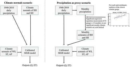
The flowchart in Figure 2 summarizes the methodology. The overall approach adopted in this study was to create, for each climate gauge available for the region, a regression equation between precipitation and these two climate variables (relative humidity, RH, and sunlight hours, SH). The regression was then used to estimate, for each month of the simulation period and for each unit-catchment of the basin, a value of each of these two variables based on the monthly total precipitation of that specific unit-catchment, which was then used to compute evapotranspiration based on the Penman-Monteith equation.

Figure 2. Overview of the methodology used, comparing the simulation scenarios with and without precipitation as proxy. RH: relative humidity; SH: sunlight hours; ST: surface average air temperature; WS: wind speed; AP: atmospheric pressure

A total of 54 climate gauges was used (Fig. 1). Monthly averages of RH and SH were correlated to monthly total precipitation, for each month of the year, and Student’s t-test for linear Pearson correlation coefficient (r) was carried out with a 0.01 significance value to select the months with statistically significant correlations. Table 1 presents daily data availability (%) for the climate variables obtained for the 54 gauges.

For each unit-catchment, the regression equation of the nearest gauge was used to compute RH and SH to calculate actual evapotranspiration in the model. For months when the test was not significant, the nearest gauge long-term climate average was used (i.e. one average value for all January months, and so on for the other months). Precipitation values equal to zero were removed from the regression in order to avoid significant correlations in very dry months.

3.3 Simulation experiments

The following simulation experiments were carried out within this study (described in Sections 4.1–4.5):

• Correlation between observed climate variables and precipitation (Section 4.1): assessment of how climate variables (SH and RH) are correlated with precipitation for the different gauges across the basin.

• Effects of climate data based on proxy on the simulated evapotranspiration (Section 4.2): comparison of calculated actual evapotranspiration (ET) based on long-term climatology and on precipitation as proxy.

• Correlation between evapotranspiration and precipitation (Section 4.3): evaluation of changes from water- to energy-limited situations on a monthly basis.

• Inter-annual variation of hydrological regime (Section 4.4): evaluation of Q and ET time series from 1950s to 1980s in scenarios with and without proxy.

• Model sensitivity to temporal resolution of climate data (Section 4.5): analysis of sensitivity of the Q and ET outputs of the hydrological model based on different temporal availability of climate data for a region with full temporal availability of daily data. The test with the Corumbá basin was performed to evaluate the added value of having more detailed information than the climate normal, which is the precipitation as proxy approach, in comparison to adopting daily data.

4 Results and discussion

4.1 Correlation between observed climate variables and precipitation

Figure 3 presents the correlation between monthly precipitation and RH and SH for Aragarças (seasonal precipitation) and Indaial (non-seasonal precipitation) gauges, for January and June. These months were chosen as representative of the precipitation seasonality (see Figure 1(a)). Aragarças gauge is located in the north of the basin and features a distinctive seasonal climatology, for which there is a strong correlation between relative air humidity and sunlight hours and monthly precipitation during rainy season (November–March), which can be checked in the January curves shown in Figure 3. For dry months (July – Southern Hemisphere winter), this correlation does not occur, mainly because of the small range of precipitation during this period, which produces the flat regression curve in Figure 3. As another example of the seasonality effect on correlations, for the Roncador gauge (Fig. 1(b)), there were only three years in the whole 17-year period with more than 0 mm in July. Also, in the tropical regions with seasonal precipitation, the relative air humidity ranged between smaller values (50–70%) in July compared to January (70–90%), while sunlight hours ranged between 0 and 7 h/d in the rainy period and >7 h/d in the dry period.

Figure 3. Correlation between climatological variables and monthly precipitation for gauges Aragarças and Indaial. The straight (blue) line refers to the linear regression. See Figure 1 for gauge locations

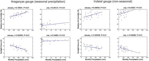
In turn, for the Indaial gauge, which has a non-seasonal precipitation behaviour, a much smaller variation exists between January and July. In this region, very similar monthly precipitation values were recorded during the year, and correlation curves are generally more steeply inclined in all months, as can be seen in the examples of Figure 3. However, this does not mean that there was always acceptable correlation in terms of p values. As one can see in Figure 3, for the Indaial gauge the correlations for RH in July and SH (h) in January had p values greater than 0.01.

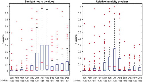
A synthesis of the regressions is presented in Figure 4, with box plots of p values for each month (a set of 54 p values, one for each gauge, was analysed for each month). These results indicate that the Brazilian summer months (January, February and March) have more significant correlations than winter months for both sunlight hours and relative humidity. Median values of p were smaller than 0.01 for all months except June, July, August, October and December for SH, and May, June, July and August for RH. The occurrence of these smaller p values was reinforced by the rainfall seasonality effects explained above, which generated flat regression curves in regions where a marked dry period occurs.

Figure 4. Box plots of p values for each month for the correlations between monthly precipitation and sunlight hours and relative humidity, based on a set of 54 p values (one for each climate gauge). Median values are displayed at the figure bottom

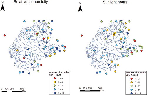
We used a simple criterion to define whether or not to use a regression equation based on a 0.01 significance level, which we understand to be a restricted value, and its applicability was validated by visual inspection of the regression lines. The regression Pearson correlation (r) obtained and associated p values for the correlations between monthly precipitation and monthly RH and SH for each gauge are presented in Appendix B (Table B1). Additionally, Figure 5 shows a map of the Paraná River Basin with all climate gauges used in this study, with the number of months for which a significant correlation (p < 0.01) between climate variables and monthly precipitation was found. Most gauges have more than six months of the year with a significant correlation.

Table B1. Main statistics for the correlations between monthly sunlight hours and precipitation for the months January and July. Pearson correlation (r) and p value are presented for each gauge

ID	Gauge name	Relative humidity regression with precipitation				Sunlight hours regression with precipitation
		r (Jan)	p (Jan)	r (Jul)	p (Jul)	r (Jan)	p (Jan)	r (Jul)	p (Jul)
1	Aragarças	0.7859	0.0000	0.3613	0.1408	−0.6099	0.0001	0.2486	0.3359
2	Araxá	0.7149	0.0000	0.1320	0.5032	−0.7699	0.0000	−0.1453	0.4695
3	Arinos	0.8897	0.0000	0.3589	0.3429	−0.8920	0.0000	−0.5380	0.1351
4	Avelar	0.4858	0.0350	0.5097	0.0307	−0.5093	0.0309	−0.3703	0.1303
5	Bambuí	0.2186	0.1874	0.2177	0.2754	−0.5178	0.0010	−0.2670	0.1782
6	Barbacena	0.5222	0.0002	0.3673	0.0197	−0.6140	0.0000	−0.1028	0.5335
7	Brasília	0.7276	0.0000	0.2706	0.2625	−0.7426	0.0000	−0.4131	0.0787
8	Campo Mourão	0.7370	0.0000	0.3608	0.0109	−0.8046	0.0000	−0.5206	0.0002
9	Campos Do Jordão	0.5687	0.0000	0.2272	0.1380	−0.1895	0.2683	−0.1509	0.4020
10	Campos Novos	0.5692	0.0002	0.5473	0.0006	−0.4132	0.0122	−0.7660	0.0000
11	Capinópolis	0.4109	0.0115	−0.1896	0.4105	−0.5980	0.0001	0.0120	0.9589
12	Castro	0.6700	0.0000	0.3598	0.0141	−0.4146	0.0164	−0.4321	0.0171
13	Catalão	0.7312	0.0000	0.2365	0.2772	−0.6418	0.0000	−0.0030	0.9894
14	Catanduva	0.5942	0.0000	0.5942	0.0001	−0.5895	0.0002	−0.5301	0.0053
15	Chapecó	0.6183	0.0002	0.6114	0.0003	−0.4731	0.0062	−0.7697	0.0000
16	Coronel Pacheco	0.4456	0.0040	0.0248	0.8910	−0.6240	0.0000	−0.2149	0.2298
17	Curitiba	0.4830	0.0004	0.5419	0.0000	−0.4992	0.0004	−0.5867	0.0000
18	Divinópolis	0.9166	0.0000	0.1978	0.5171	−0.2275	0.4148	−0.6882	0.0093
19	Franca	0.6464	0.0000	0.7144	0.0000	−0.4865	0.0017	−0.1912	0.3029
20	Goiás	0.5749	0.0000	0.3055	0.2035	−0.7355	0.0000	−0.3812	0.1452
21	Guarulhos	0.5059	0.0071	0.3980	0.0440	−0.5216	0.0053	−0.3263	0.1114
22	Indaial	0.4966	0.0033	0.4060	0.0172	−0.3631	0.0378	−0.5659	0.0006
23	Ipameri	0.5714	0.0005	0.2383	0.3740	−0.6070	0.0006	0.2588	0.3717
24	Irati	0.5113	0.0004	0.5778	0.0000	−0.4538	0.0020	−0.5760	0.0001
25	Iraí	0.4553	0.0019	0.4304	0.0028	−0.4333	0.0029	−0.5943	0.0000
26	Ituiutaba	0.5508	0.0029	−0.1013	0.8113	−0.6143	0.0051	−0.1416	0.7620
27	Itumbiara	0.7475	0.0004	−0.0871	0.8109	−0.5030	0.0334	0.1337	0.7128
28	Ivinhema	0.2397	0.1790	0.1122	0.5550	−0.7446	0.0000	−0.4036	0.0179
29	Jataí	0.5354	0.0016	0.2848	0.2372	−0.5520	0.0013	−0.3029	0.2372
30	João Pinheiro	0.6759	0.0000	0.3399	0.1217	−0.4992	0.0250	0.0966	0.7537
31	Juiz De Fora	0.4286	0.0024	0.4464	0.0027	−0.5785	0.0000	−0.3628	0.0155
32	Lavras	0.6030	0.0000	0.5140	0.0037	−0.6620	0.0000	−0.1968	0.2973
33	Londrina	0.5867	0.0000	0.3310	0.0246	−0.6822	0.0000	−0.5252	0.0008
34	Machado	0.4325	0.0038	0.4346	0.0064	−0.5298	0.0003	−0.3872	0.0163
35	Maringá	0.5793	0.0001	0.4961	0.0018	−0.7732	0.0000	−0.5020	0.0055
36	Mirante Santana	0.0489	0.7362	0.4956	0.0003	−0.2363	0.1653	−0.3103	0.0696
37	Nhum	0.6499	0.0026	−0.0967	0.7424	−0.7264	0.0004	−0.1979	0.5170
38	Paracatu	0.6247	0.0001	0.5079	0.0637	−0.8192	0.0000	−0.5897	0.0265
39	Paranaguá	0.3500	0.0148	0.3879	0.0064	−0.0881	0.5886	−0.5911	0.0000
40	Paranaíba	0.5594	0.0007	0.4657	0.0144	−0.6120	0.0002	−0.2817	0.1545
41	Patos De Minas	0.6368	0.0000	0.1624	0.4279	−0.6839	0.0000	0.0081	0.9688
42	Pirenópolis	0.7999	0.0000	0.4626	0.0825	−0.7517	0.0000	0.2347	0.3997
43	Poços De Caldas	0.3765	0.0166	0.2683	0.1377	−0.7600	0.0000	−0.3873	0.0615
44	Presidente Prudente	0.7316	0.0000	0.2791	0.0634	−0.7396	0.0000	−0.3137	0.0358
45	Resende	0.4921	0.0017	0.4908	0.0013	−0.2954	0.0642	−0.3869	0.0136
46	Rio Verde	0.5842	0.0011	0.2432	0.2881	−0.3491	0.0686	0.0011	0.9963
47	Roncador	0.6776	0.0028	−0.8481	0.3556	−0.7689	0.0003	−0.9653	0.1681
48	Sorocaba	0.7389	0.0000	0.4987	0.0081	−0.6906	0.0004	−0.4593	0.0275
49	São Carlos	0.5299	0.0001	0.2659	0.0929	−0.6130	0.0002	−0.2364	0.2449
50	São Lourenço	0.2691	0.0739	0.3498	0.0215	−0.3017	0.0493	−0.4496	0.0028
51	São Simão	0.5544	0.0001	0.4711	0.0037	−0.5645	0.0001	−0.2587	0.1276
52	Taubaté	0.5365	0.0019	0.4730	0.0047	−0.4610	0.0091	−0.0366	0.8451
53	Uberaba	0.2788	0.0669	−0.0821	0.7028	−0.7425	0.0000	0.0506	0.8102
54	Unaí	0.7272	0.0000	0.0013	0.9969	−0.8379	0.0000	−0.3199	0.3376

Figure 5. Number of months of the year with p < 0.01 for each gauge for relative air humidity and sunlight hours

The results presented in this section indicate that it is possible to use regression curves between monthly precipitation and climate variables to estimate monthly values of the latter for many months of the year across the whole Paraná Basin. These regressions are used in the next sections to improve model estimates of discharge and evapotranspiration time series by using a better temporal resolution of climate data.

4.2 Effects of climate data based on proxy on the simulated evapotranspiration

Time series of relative air humidity, sunlight hours and actual evapotranspiration computed from climate normals (constant values for all months) or based on regression with precipitation (one different value for each month) are presented in Figures 6 and 7 for the unit-catchments of Brasília city and Itaipu Dam (see Figure 1), which are representative of seasonal and non-seasonal precipitation regions, respectively.

Figure 6. Daily relative air humidity and sunlight hours for Brasilia (north of the basin) and Itaipu Dam (southern region), as computed from precipitation as proxy or only from climate averages

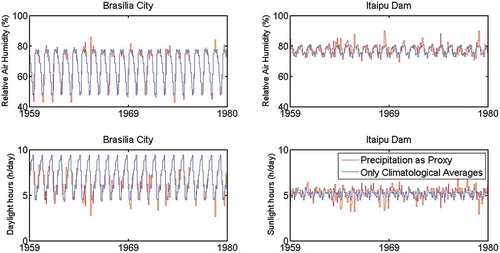
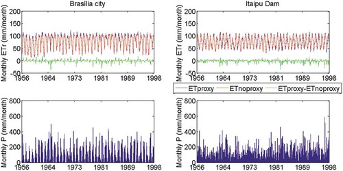
Figure 7. Monthly actual evapotranspiration (ET), with the two types of computation of climate variables, Precipitation as Proxy (ETproxy, blue) and Only Climatological Averages (ETnoproxy, red), and the difference between them (ETproxy − ETnoproxy, green), for Brasília city and Itaipu Dam, and monthly precipitation (P) for the same locations

For the Brasília location, the inclusion of precipitation as a proxy led to alterations mainly in rainy periods, with higher values of RH and smaller ones of SH, while values of RH (sunlight hours) based on climate normals ranged from 48% (4.5 h) to 78% (9.4 h), and using the regression with precipitation they varied between 43% (0 h) and 100% (9.4 h). In the southern region with non-seasonal precipitation, variation in both climate variables occurred throughout the whole period. Relative air humidity (sunlight hours) values varied in a narrower range, between 73% (4.5 h) and 81% (5.8 h), while the use of precipitation as proxy widened the ranges, with values from 70% (1.3 h) to 97% (6.6 h).

Generally, the incorporation of precipitation as proxy in the simulation was able to change the evapotranspiration rates, but differences were smaller than the seasonal ranging of evapotranspiration for both locations. Differences were higher during wetter periods, when precipitation altered climate variables most, and the maximum difference was 38 mm/month for Brasília and 35 mm/month for Itaipu, when evapotranspiration based on proxy was smaller than the other scenario.

4.3 Correlation between evapotranspiration and precipitation

An interesting way to understand how precipitation affects evapotranspiration rates and hydrological processes across the basin is to evaluate changes in the precipitation–evapotranspiration relationship through the annual cycle. Figures 8 and 9 present the correlation between monthly precipitation and model-calculated monthly actual evapotranspiration for each month of the year for Brasília city and Itaipu Dam, considering the scenarios with and without precipitation as proxy. Different correlation slopes were detected for each month, which is related to the local seasonal cycle of climate. As showed by Collischonn and Tucci (2014), potential evapotranspiration is inversely correlated with precipitation, since no soil moisture restriction is considered in its computation. When it comes to actual evapotranspiration, however, available soil moisture becomes an important constraint in some months. In Brazilian Cerrado regions, evapotranspiration has been observed to be reduced in dry periods due to decreasing soil water availability, in contrast to the Amazon region, for instance, where evapotranspiration is more dependent on incoming solar radiation and has a peak during the dry season (da Rocha et al. 2009).

Figure 8. Relationship between monthly precipitation and simulated monthly evapotranspiration for Brasília City (northern region) for the simulation period 1940–2010

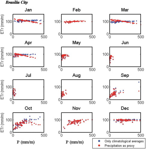
Figure 9. Relationship between monthly precipitation and simulated monthly evapotranspiration for Itaipu Dam (southern region) for the simulation period 1940–2010

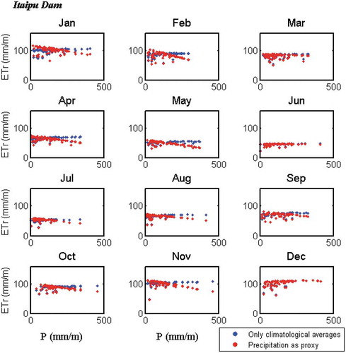
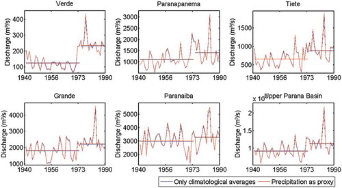
Figure 10. Long-term variation in calculated annual average discharge with and without precipitation as proxy. Horizontal lines indicate average values pre- and post-1973

Considering the precipitation as proxy scenario, for Brasília city, there is a clear change in the slope of the correlation line throughout the year. During the rainy season, evapotranspiration is inversely related to precipitation, since soil moisture is available and the increasing sunlight hours are the main constraints for evapotranspiration. In the beginning of the dry period (May) the relationship tends toward constant evapotranspiration rates, while in the driest months (June–August), the variation in evapotranspiration rates is possibly related to different antecedent soil moisture conditions from previous months. Finally, during the beginning of the wet period (September–October), there is a positive relationship, where more precipitation tends toward higher evapotranspiration rates, until December, when the slope changes back to negative and the cycle repeats. The scenario with only climatological variables was not able to represent the variation in slope for the annual cycle. Finally, it must be noted that, for regions with seasonal precipitation, fewer months showed significant correlation between climatological variables and monthly precipitation in comparison to non-seasonal precipitation regions.

For the Itaipu Dam location, actual evapotranspiration was negatively correlated to precipitation in most months in the scenario using precipitation as proxy, while the scenario without proxy led to very small variations in evapotranspiration. This behaviour happens because, after a given turning point, increasing precipitation leads to fewer sunlight hours, decreasing evapotranspiration.

These results indicate that, throughout the year, regions may change from being soil moisture limited to energy limited (especially for northern, seasonal precipitation regions), as revealed by the different correlations found between actual evapotranspiration and precipitation. The use of only climatological averages does not allow such interpretations. Differences between scenarios with climatological averages and using a proxy are larger during wetter months due to the influence of cloud cover (e.g. monthly precipitation totals >200 mm for January in Brasília city). For months with a positive correlation between evapotranspiration and precipitation, much more precipitation than occurred in the simulated period would be needed to turn this relationship into a negative one. The results presented here are interesting in that they show the potential of including monthly variation in climatological variables in hydrological studies. One additional advantage of using precipitation as a proxy is that it is possible to consider differences between climate data in different unit-catchments/regions by using a dense network of precipitation gauges, since rainfall gauge networks are typically denser than networks of climate gauges.

4.4 Inter-annual variation of Upper Paraná River hydrological regime

An important scientific debate on the Paraná River Basin is related to significant changes in its hydrological regime during recent decades (García and Vargas 1998). Discharge was observed to increase significantly from the 1970s onward, and causes for this nonstationarity were attributed to land use and land cover change, and alterations in the climate regime (Krepper et al. 2008, Bayer 2014, Lee et al. 2018). The change in the Paraná River mean discharges was so significant that it led to an increase in the number of turbines required at the Itaipu Dam, from the 18 initially projected to a total of 20 today. Bayer (2014) estimated that 39% of this increase in discharge was due to deforestation in the Paraná Basin, and 61% due to increases in precipitation.

Although previous studies have shown the effects of changes in precipitation in the Paraná River Basin response, they have not explored the inter-annual variation of climate variables (such as sunlight hours and relative humidity), and the potential effect that changes in precipitation have on evapotranspiration to alter these climate variables. Thus, in this section, the estimation of monthly climate variables based on precipitation as proxy is evaluated in terms of its impact on annual changes of both discharge and evapotranspiration. The model was run for the studied basin considering the period from 1 January 1940 to 31 December 2010.

Figures 10 and 11 show temporal series of discharge and evapotranspiration, respectively, for six selected sub-basins of the Paraná River Basin: Verde, Paranapanema, Tietê, Grande, Paranaíba and the whole Upper Paraná River Basin. The results are displayed for simulation scenarios with and without precipitation as proxy. It is observed that the scenario with precipitation as proxy led to less calculated evapotranspiration; this in accordance with the results from Section 4.3, where it was shown that wet months tended to present a negative correlation between precipitation and evapotranspiration, which could not be represented in the scenario using climate normals. Smaller evapotranspiration rates (Fig. 11) generated higher annual discharges (Fig. 10).

Figure 11. Long-term variation in calculated annual evapotranspiration with and without precipitation as proxy. Horizontal lines indicate average values pre- and post-1973

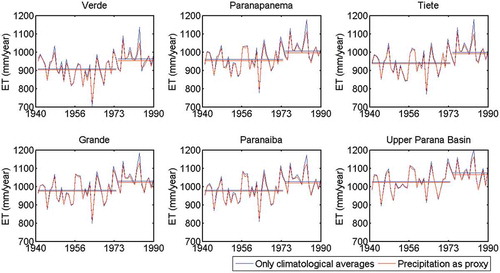
Long-term averages for periods pre- and post-1973, which roughly define the period from which important hydrological changes were observed in the basin, are also plotted as horizontal lines in Figures 10 and 11. Average values show smaller evapotranspiration rates and higher discharges after 1973.

For the whole Upper Paraná Basin, post-1973 the scenario with (without) proxy led to a long-term average evapotranspiration of 1066 (1074) mm/year, while pre-1973 it was 1023 (1027) mm/year. Similar behaviours were observed for the other sub-basins. For discharge, in the Upper Paraná Basin the post-1973 period had an average discharge of 11 460 (11 260) m³/s, against 9236 (9148) m³/s for the pre-1973 period. A mean difference of ~200 m³/s occurred after 1973, and ~88 m³/s before 1973, and this increase in the difference value may be explained by the higher precipitation rates after 1973 that led to fewer sunlight hours. This analysis, however, indicates that the long-term effect of precipitation on sunlight hours and relative humidity explains a small part of the increase in discharge (and decrease in evapotranspiration) in the basin, given the relatively small differences between scenarios with and without precipitation as proxy.

In the Paraná River Basin, discharge has increased with time since the 1970s due mainly to land cover changes and increases in precipitation volumes (Bayer 2014). Our results suggest that an additional source of increasing discharge is the reduction in sunlight hours and increase in relative humidity due to increasing precipitation, although this effect is certainly less important than the other two, if compared to MGB simulations by Bayer (2014) for instance.

Regarding evapotranspiration computation with the Penman-Monteith equation, as in the MGB model, it would also be interesting to evaluate impacts from changes in surface air temperature. However, estimates of the temporal variation of this variable were not considered in this study, given the poor correlation with precipitation found by Collischonn and Tucci (2014). A further development of this study could involve the simulation of the nonstationary hydrological regime in the basin by considering changes of land use, precipitation and climate variables (i.e. beyond sunlight hours and relative humidity, such as temperature).

4.5 Model sensitivity to temporal resolution of climate data

In the previous sections, evaluation was carried out through comparisons between the MGB model simulations using long-term averages of climate variables (relative air humidity, sunlight hours, air temperature, wind speed, air pressure – RH, SH, ST, WS and AP, respectively) and monthly values of climate variables based on precipitation as proxy. The latter is an interesting approach for poorly gauged basins, where daily climate data are typically not available, and monthly estimates are actually better than long-term averages. However, it is important to understand how model outputs based on monthly climate values compare to those using daily data, which would be the ideal scenario (for smaller basins, hourly observed data could also be important). Thus, in this section, we evaluated the effect on model estimates of adopting the following three approaches of data temporal resolution:

1. daily data for RH, SH, ST, WS, AP (reference scenario);

2. monthly averages of RH and SH and climate normals for ST, WS and AP (similar to using precipitation as proxy); and

3. long-term monthly climate average for RH, SH, ST, WS, AP.

The sub-basin of the Corumbá River (before its confluence with the Paranaíba River in the northern Paraná River Basin; Figure 1(b)) was selected as the test basin, because of the location of the Roncador climate gauge, which had full availability of climate variables for a satisfactory period of time. The period 1 January 1995 to 31 December 2000 (6 years) was identified as having no failures (complete time series with observed data). This short period of full data availability also shows the relevance of developing methods for estimating temporal variability of climate variables, such as the use of precipitation as proxy, as proposed by Collischonn and Tucci (2014) and this study, since no other gauging location had an equivalent or better time series.

Figure 12(a) shows the simulated discharge at the Corumbá sub-basin outlet, and Figure 12(b) and (c) shows the calculated evapotranspiration for scenarios a, b and c. The results indicate small differences between the three scenarios for discharge, but large ones for simulated actual evapotranspiration. The use of monthly values (scenarios b and c) generally filtered out important daily variations, but higher errors occurred when using long-term averages of climate data. The usage of climate normals (scenario c) led to even more attenuated monthly evapotranspiration rates, with less extreme values than the proxy scenario (scenario b). Using precipitation as proxy seemed a good approach for estimating monthly evapotranspiration values, and this technique seems preferable to simply adopting long-term averages.

Figure 12. (a) Discharge at the Corumbá River sub-basin outlet for scenarios a–c; and (b) daily and (c) monthly evapotranspiration for the Corumbá River sub-basin. See Figure 1(b) for the sub-basin location

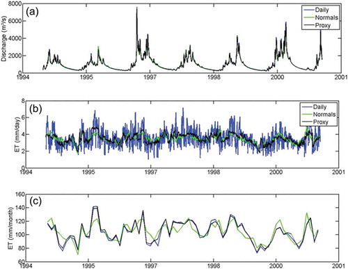
These results also indicate that evapotranspiration is more sensitive to the temporal resolution of climate data than is discharge. Actually, to deal with possible over- or underestimation of discharge, the modeller may use overparameterization to overcome errors in evapotranspiration and reach satisfactory modelled discharges in typical hydrological model applications which are focused mainly on discharge estimation. This procedure could be avoided with a more correct temporal resolution of input climate variables.

5 Conclusions

In this study, multiple analyses were carried out to elucidate the effect of precipitation on climate variables that ultimately influence evapotranspiration and water budget components in large river basins. The study case was the Paraná River Basin, a prominent case of perceptible changes in hydrological regime. Monthly precipitation was used as a proxy of monthly values of sunlight hours and relative humidity, and these new estimates were then used as input data for a MGB model application. Results were generally compared to a simulation scenario using long-term climate averages as input.

In the “precipitation as proxy” approach proposed here, precipitation affects evapotranspiration in two ways – by altering relative humidity and sunlight hours and by controlling the soil moisture cycle, which limits water uptake by plants during dry periods. By applying precipitation as proxy, it is possible to take advantage of heterogeneity of precipitation across the basin, using a generally more distributed precipitation gauging network to estimate climate data.

The main conclusions from this work are:

• Precipitation can be used as a proxy of climate variables (i.e. sunlight hours and relative humidity), which is useful for improving their temporal resolution, from long-term climate averages (i.e. climate normals) towards monthly values.

• Using precipitation as proxy to estimate monthly values of sunlight hours and relative humidity leads to a better estimation of monthly evapotranspiration, in comparison to using only long-term average values, when compared to evapotranspiration estimated using daily climate data (study case in the Corumbá River Basin, a sub-basin of the Paraná).

• Differences between scenarios considering precipitation or not as a proxy for climate variables occurred mainly in the wetter months, so that the correlation between monthly precipitation and monthly evapotranspiration changed from positive to negative in the evaluated locations (Brasília and Itaipu Dam) of the Paraná River Basin.

• For the studied region with seasonal precipitation (Brasília city) during the rainy period, a negative correlation was found between monthly precipitation and evapotranspiration in wetter months, since soil moisture is usually available and the main constraint is radiation availability.

• For the studied region with non-seasonal precipitation (Itaipu Dam), a negative correlation between monthly precipitation and evapotranspiration was found for most months.

• Analysis of the long-term changes of the hydrological regime of the Upper Paraná River Basin showed that the effect of a changing precipitation on relative humidity and sunlight hours has a minor effect on the nonstationarity of hydrological fluxes.

Given our results, the effect of a changing precipitation on relative humidity and sunlight hours seems to have a minor effect on hydrological fluxes if compared to other alterations in the basin, such as changes in land use and precipitation itself (Bayer 2014, Lee et al. 2018). To further understand these mechanisms, a continuation of the presented research could include: (1) combining land use changes (e.g. using inter-decadal land cover maps) and the precipitation as proxy approach to run the hydrological model and assess the streamflow time series; and (2) comparison of the obtained results with the use of climate variables from long-term re-analysis data.

Disclosure statement

No potential conflict of interest was reported by the authors.

Additional information

Funding

The authors would like to thank CNPq for funding this research [grant number: 141161/2017-5].

Notes

¹ https://www.ufrgs.br/lsh/products/remote-sensing/simplified-hydrological-response-units-map-for-south-america/.

Appendix A.

Model calibrated parameters and model performance

All model calibrated parameters for the hydrological vertical balance (soil water budget) are presented in Table A1 (for more details on model parameterization see Collischonn et al. 2007). Within a given unit-catchment, there is one computation of rainfall–runoff processes for each existent HRU. Also, within each of the six sub-basins (Fig. 1(d)), the same rainfall–runoff parameters are applied to each HRU type. Then, for example, all “Forest with shallow soil” HRUs in the unit-catchments of sub-basin 1 will have the same rainfall–runoff parameters. The only exception is made for parameters CS, CI and CB, which are related to surface, sub-surface and baseflow linear reservoirs (hillslope propagation module within catchment) of the unit-catchments (as described in Section 3.1.1), and are defined as constant for all unit-catchments within a sub-basin.

Table A2 presents model validation for the 26 gauges displayed in Figure A1 through the KGE performance metric, showing a satisfactory model performance.

Table A1. Model calibrated parameters for rainfall–runoff processes: Wm: maximum water storage in the soil of each HRU; b: parameter from the variable contributing area model for runoff generation; Kbas and Kint: equivalent hydraulic conductivities for baseflow and subsurface flow;; and CS, CI and CB: related to residence time within surface, subsurface and baseflow linear reservoirs, respectively. The HRUs adopted in this study are: Forest_Deep: forest with deep soil; Forest_Shallow: forest with shallow soil; Agric_Shallow: agriculture with shallow soil; Agric_Deep: agriculture with deep soil; Grass_Shallow: grasslands with shallow soil; Grass_Deep: grasslands with deep soil; Floodplain: floodplain areas adjacent to rivers; and Urban: urban areas

Sub-basins	Wm (mm)	b (-)	Kbas (mm d^−1)	Kint (mm d^−1)
Sub-basin 1: Granitoid, volcanic and some metamorphic rock
Forest_Deep	500	0.1	1.5	5
Forest_Shallow	700	0.1	2.5	10
Agric_Shallow	500	0.1	1.5	5
Agric_Deep	700	0.1	2.5	10
Grass_Shallow	500	0.1	1.5	5
Grass_Deep	700	0.1	2.5	10
Floodplain	300	0.1	1	5
Urban	100	0.1	0.1	5
CS	15
CI	150
CB	5000
Sub-basin 2: Basalt and dacite
Forest_Deep	300	0.5	0.3	4
Forest_Shallow	400	0.5	0.8	4
Agric_Shallow	300	0.5	0.3	4
Agric_Deep	400	0.5	0.8	4
Grass_Shallow	300	0.5	0.3	4
Grass_Deep	400	0.5	0.8	4
Floodplain	400	0.5	0.8	4
Urban	100	0.5	0.1	4
CS	10
CI	100
CB	5000
Sub-basin 3: Sandstone and conglomerate
Forest_Deep	1000	0.1	2	20
Forest_Shallow	1200	0.1	3	30
Agric_Shallow	1000	0.1	2	20
Agric_Deep	1200	0.1	3	30
Grass_Shallow	1000	0.1	2	20
Grass_Deep	1200	0.1	3	30
Floodplain	300	0.1	3	30
Urban	100	0.1	0.1	20
CS	10
CI	100
CB	8000
Sub-basin 4: Sandstone, mudstone and conglomerate
Forest_Deep	700	0.1	1.5	35
Forest_Shallow	800	0.1	2	35
Agric_Shallow	700	0.1	1.5	35
Agric_Deep	800	0.1	2	35
Grass_Shallow	700	0.1	1.5	35
Grass_Deep	800	0.1	2	35
Floodplain	200	0.1	1.5	2
Urban	100	0.1	0.1	2
CS	18
CI	180
CB	4000
Sub-basin 5: Sandstone, diamictite, shale, rhythmite, siltstone and conglomerate
Forest_Deep	300	0.5	0.5	12
Forest_Shallow	400	0.5	1	17
Agric_Shallow	300	0.5	0.5	12
Agric_Deep	400	0.5	1	17
Grass_Shallow	300	0.5	0.5	12
Grass_Deep	400	0.5	1	17
Floodplain	100	0.5	0.5	10
Urban	100	0.5	0.1	10
CS	10
CI	100
CB	5000
Sub-basin 6: Basalt and dactite with sandstone outcrops
Forest_Deep	900	0.1	1.5	10
Forest_Shallow	1000	0.1	2.5	10
Agric_Shallow	900	0.1	1.5	10
Agric_Deep	1000	0.1	2.5	10
Grass_Shallow	900	0.1	1.5	10
Grass_Deep	1000	0.1	2.5	10
Floodplain	300	0.1	1	10
Urban	100	0.1	0.1	10
CS	10
CI	100
CB	5000

Table A2. Performance metrics (KGE) after model validation for the 26 gauges presented in Figure A1

Gauge ID	Gauge name	KGE
1	EngenheiroAmorim	0.507
2	Pires do Rio	0.614
3	Ponte Meia Ponte	0.886
4	Fazenda Santa Maria	0.808
5	Maurilândia	0.71
6	Abaixo Barra do Rio Verde	0.833
7	Clube de Regatas	0.719
8	Uhe Marimbondo	0.601
9	Porto Cunha Bueno	0.754
10	Passagem	0.577
11	Uhe Marimbondo Passagem	0.596
12	Ponte Joaquim Justino	0.507
13	Artemis	0.775
14	Fazenda Ipacarai	0.484
15	União da Vitória	0.687
16	Água Vermelha	0.881
17	Ibitinga	0.91
18	Itaipi	0.891
19	Jupia	0.829
20	Marimbondo	0.876
21	N Avanhandava	0.902
22	P Primavera	0.827
23	Porto Ivinhema	0.504
24	Porto Paraiso do Norte	0.562
25	Rosana	0.775
26	Salto Caxias	0.807

Figure A1. Discharge gauges used for model validation. KGE performance metrics are presented in Table A2

Appendix B.

Correlation between precipitation and climate variables

Table B1 presents, for each gauge, the obtained regression Pearson correlation and associated p values for the correlations between monthly precipitation and monthly relative humidity and sunlight hours. Results are presented only for January and July for brevity.

References

- Allen, R.G., et al., 1998. Crop evapotranspiration. Guidelines for computing crop water requirements. FAO Irrigation and Drainage Paper. Rome, Italy: Food and Agricultural Organization of the United Nations.
- Alvares, C.A., et al., 2013. Köppen’s climate classification map for Brazil. Meteorologische Zeitschrift, 22 (6), 711–728. doi:10.1127/0941-2948/2013/0507
- Bastiaanssen, W.G.M., et al., 1998. A remote sensing surface energy balance algorithm for land (SEBAL): part 2 validation. Journal of Hydrology, 212–213, 213–229.
- Bayer, D., 2014. Efeitos das mudanças de uso da terra no regime hidrológico de bacias de grande escala. PhD Thesis. Instituto de Pesquisas Hidráulicas (IPH), Porto Alegre, Brazil.
- Beven, K., 1979. A sensitivity analysis of the Penman-Monteith actual evapotranspiration estimates. Journal of Hydrology, 44, 169–190. doi:10.1016/0022-1694(79)90130-6
- Beven, K., 2006. A manifesto for the equifinality thesis. Journal of Hydrology, 320, 18–36. doi:10.1016/j.jhydrol.2005.07.007
- Blaney, H.F. and Criddle, W.D., 1950. Determining water needs from climatological data. US Department of Agriculture Soil Conservation Service. SOS–TP, USA.
- Bonan, G., 2008. Ecological climatology: concepts and applications. 2nd edn. Cambridge, UK: Cambridge University Press, 550 pp.
- Budyko, M.I., 1958. The heat balance of the Earth’s surface. Translated from Russian by N.A. Stepanova. Washington, DC: Office of the Technical Service, US Deparment of Commerce, 259.
- Collischonn, B. and Collischonn, W., 2016. Rainfall as proxy for evapotranspiration predictions. Proceedings of the International Association of Hydrological Sciences, 374, 35–40. doi:10.5194/piahs-374-35-2016
- Collischonn, B. and Tucci, C.E.M., 2014. Relações regionais entre precipitação e evapotranspiração mensais. Revista Brasileira de Recursos Hídricos, 19 (3), 205–214. doi:10.21168/rbrh.v19n3.p205-2014
- Collischonn, W., et al., 2007. The MGB-IPH model for large-scale rainfall—runoff modelling. Hydrological Sciences Journal, 52, 878–895. doi:10.1623/hysj.52.5.878
- Corbari, C., et al., 2014. Evapotranspiration estimate from water balance closure using satellite data for the Upper Yangtze River basin. Hydrology Research, 45 (4–5), 603–614. doi:10.2166/nh.2013.016
- da Rocha, H.R., et al., 2009. Patterns of water and heat flux across a biome gradient from tropical forest to savanna in Brazil. Journal of Geophysical Research, 114, G00B12. doi:10.1029/2007JG000640
- Droogers, P. and Allen, R.G., 2002. Estimating reference evapotranspiration under inaccurate data conditions. Irrigation and Drainage Systems, 16 (1), 33–45. doi:10.1023/A:1015508322413
- Empresa de Pesquisa Energética (EPE), 2015. Brazilian energy balance. Rio de Janeiro, Brazil. 291 pp.
- Fan, F., et al., 2014. Ensemble streamflow forecasting experiments in a tropical basin: the São Francisco river case study. Journal of Hydrology, 519, 2906–2919. doi:10.1016/j.jhydrol.2014.04.038
- Fan, F.M., et al., 2015. A hydrological response units map for all South America. XXI Simpósio Brasileiro de Recursos Hídricos, Brasília, Brazil. Anais do XXI Simpósio Brasileiro de Recursos Hídricos.
- García, N.O. and Vargas, W.M., 1998. The temporal climatic variability in the ‘Río De La Plata’ Basin displayed by the river discharges. Climatic Change, 38, 359–379. doi:10.1023/A:1005386530866
- Gong, L., et al., 2006. Sensitivity of the Penman-Monteith reference evapotranspiration to key climatic variables in the Changjiang (Yangtze River) basin. Journal of Hydrology, 329 (3–4), 620–629. doi:10.1016/j.jhydrol.2006.03.027
- González-Dugoa, M.P., et al., 2013. Monitoring evapotranspiration of irrigated crops using crop coefficients derived from time series of satellite images. II. Application on basin scale. Agricultural Water Management, 125, 81–91. doi:10.1016/j.agwat.2012.11.005
- Guitjens, J., 1982. Models of alfalfa yield and evapotranspiration. Journal of the Irrigation and Drainage Division ASCE, 108 (3), 212–222.
- Harbeck, G.E., Jr., 1962. A practical field technique for measuring reservoir evaporation utilizing mass-transfer theory. US Geological Survey, Paper 272-E, 101–105.
- Hrachowitz, M., et al., 2013. A decade of Predictions in Ungauged Basins (PUB)—a review. Hydrological Sciences Journal, 58 (6), 1198–1255. doi:10.1080/02626667.2013.803183
- Jung, C.-G., Lee, D.-R., and Moon, J.-W., 2016. Comparison of the Penman-Monteith method and regional calibration of the Hargreaves equation for actual evapotranspiration using SWAT-simulated results in the Seolma-cheon basin, South Korea. Hydrological Sciences Journal, 61 (4), 793–800. doi:10.1080/02626667.2014.943231
- Jury, M., 2017. Evaluation of satellite-model proxies for hydro-meteorological services in the upper Zambezi. Journal of Hydrology: Regional Studies, 13, 91–109.
- Krepper, C.M., Garcia, N.O., and Jones, P.D., 2008. Low-frequency response of the upper Paraná basin. International Journal of Climatology, 28, 351–360. doi:10.1002/joc.1535
- Lee, E., et al., 2018. Land cover change explains the increasing discharge of the Paraná River. Regional Environmental Change, 18, 1871–1881. doi:10.1007/s10113-018-1321-y
- Li, B., Chen, F., and Liu, X., 2016. Sensitivity of the Penman-Monteith reference evapotranspiration to sunshine duration in the Upper Mekong River Basin. Hydrological Sciences Journal, 62 (5), 830–842. doi:10.1080/02626667.2016.1243286
- Moiwo, J.P., et al., 2011. Comparison of evapotranspiration estimated by ETWatch with that derived from combined GRACE and measured precipitation data in Hai River Basin, North China. Hydrological Sciences Journal, 56 (2), 249–267. doi:10.1080/02626667.2011.553617
- Monteith, J.L., 1965. Evaporation and environment. Symposia of the Society for Experimental Biology, 19, 205–234.
- Oudin, L., et al., 2010. Estimating potential evapotranspiration without continuous daily data: possible errors and impact on water balance simulations. Hydrological Sciences Journal, 55 (2), 209–222. doi:10.1080/02626660903546118
- Paiva, R., et al., 2013. Large scale hydrologic and hydrodynamic modeling of the Amazon River basin. Water Resources Research, 49, 1226–1243. doi:10.1002/wrcr.20067
- Penman, H.L. and Long, I.F., 1960. Weather in wheat. Quarterly Journal of the Royal Meteorological Society, 86, 16–50. doi:10.1002/qj.49708636703
- Pontes, P., et al., 2017. MGB-IPH model for hydrological and hydraulic simulation of large floodplain river systems coupled with open source GIS. Environmental Modelling & Software, 94, 1–20. doi:10.1016/j.envsoft.2017.03.029
- Priestley, C.H.B. and Taylor, R.J., 1972. On the assessment of surface heat flux and evaporation using large-scale parameters. Monthly Weather Review, 100, 81–92. doi:10.1175/1520-0493(1972)100<0081:OTAOSH>2.3.CO;2
- Rasmusson, E., et al., 1993. Climatology. In: D. Maidment, ed. Handbook of hydrology (pp. 2.30–2.32). New York: McGraw-Hill.
- Ruhoff, A.L., et al., 2013. Assessment of the MODIS global evapotranspiration algorithm using eddy covariance measurements and hydrological modelling in the Rio Grande basin. Hydrological Sciences Journal, 58 (8), 1658–1676. doi:10.1080/02626667.2013.837578
- Seevers, P.M. and Ottmann, R.W., 1994. Evapotranspiration estimation using a normalized difference vegetation index transformation of satellite data. Hydrological Sciences Journal, 39 (4), 333–345. doi:10.1080/02626669409492754
- Seiller, G. and Anctil, F., 2015. How do potential evapotranspiration formulas influence hydrological projections? Hydrological Sciences Journal, 61 (12), 2249–2266. doi:10.1080/02626667.2015.1100302
- Su, H., et al., 2005. Modeling evapotranspiration during SMACEX: comparing two approaches for local- and regional-scale prediction. Journal of Hydrometeorology, 6, 910–922. doi:10.1175/JHM466.1
- Thornthwaite, C.W., 1948. An approach toward a rational classification of climate. Geographical Review, 38 (1), 55–94. doi:10.2307/210739
- Walsh, P.D. and Lawler, D.M., 1981. Rainfall seasonality: description, spatial patterns and change through time. Weather, 36, 201–208. doi:10.1002/wea.1981.36.issue-7
- Wang, Q., et al., 2011. Monthly versus daily water balance models in simulating monthly runoff. Journal of Hydrology, 404, 166–175. doi:10.1016/j.jhydrol.2011.04.027
- Wilby, R.L., et al., 2000. Hydrological responses to dynamically and statistically downscaled climate model output. Geophysical Research Letters, 27 (8), 1199–1202. doi:10.1029/1999GL006078
- Wood, A.W., et al., 2004. Hydrologic implications of dynamical and statistical approaches to downscaling climate model outputs. Climatic Change, 62, 189–216. doi:10.1023/B:CLIM.0000013685.99609.9e
- Zhang, L., et al., 2008. Water balance modeling over variable time scales based on the Budyko framework – model development and testing. Journal of Hydrology, 360, 117–131. doi:10.1016/j.jhydrol.2008.07.021