On the correlation between precipitation and potential evapotranspiration climate change signals for hydrological impact analyses

ABSTRACT

State-of-the-art hydrological climate impact assessment involves ensemble approaches to address uncertainties. For precipitation, a wide range of climate model runs is available. However, for particular meteorological variables used for the calculation of potential evapotranspiration (ET_o), availability of climate model runs is limited. It is preferred that climate model runs are considered coupled when calculating changes in precipitation and ET_o amounts, in order to preserve the internal physical consistency. This results in constraints on the maximum ensemble size. In this paper, we investigate the correlation between climate change signals of precipitation and ET_o. It is found that, for two medium-sized catchments in Belgium, uncoupling climate model runs used for calculation of change signals of precipitation and ET_o amounts does not result in a significant bias for changes in extreme flow. With these results, future impact studies can be conducted with larger ensemble sizes, resulting in a more complete uncertainty estimation.

KEYWORDS:

• climate change
• extreme flows
• impact study
• ensembles
• uncertainty

Editor R. Woods Associate editor S. Huang

Introduction

The main challenges in climate change impact analyses involve quantification and incorporation of uncertainties. This challenge manifests at different stages of a climate impact analysis and is tackled by climate model developers, climate change impact modellers, policy makers and adaptation planners (Hawkins and Sutton 2009, Katz et al. 2013, Kunreuther et al. 2014, Patt and Weber 2014, Drouet et al. 2015, Ekström et al. 2016, McMillan et al. 2017).

The uncertainty in the future climate system is characterized through the representative concentration pathways (RCPs), the climate model uncertainty and the stochastic uncertainty (Hawkins and Sutton 2009, Moss et al. 2010, van Vuuren et al. 2011, Fatichi et al. 2016, Hosseinzadehtalaei et al. 2017a, Van Uytven and Willems 2018). Through a cooperation amongst 20 climate modelling groups in the Coupled Model Intercomparison Project Phase 5 (CMIP5, Taylor et al. 2012), a large set of climate model runs became available; this set consists of various climate models, forced by the different RCPs and run with various sets of initial conditions.

For hydrological modelling of climate change impacts, the spatial and/or temporal resolution of the global climate model data output mismatches the resolutions of interest. Another problem is that the climate model output data are often significantly biased. Although dynamical downscaling increases the resolution, biased output remains persistently produced (Jacob et al. 2014, Maraun 2016). Therefore, statistical downscaling and bias correction methods are applied, where methods differ in underlying assumptions, strengths and limitations (Fowler et al. 2007, Maraun et al. 2010, Chen et al. 2011, Bürger et al. 2013, Ekström et al. 2015, Sunyer et al. 2015). Similarly to the climate models, an ensemble of statistical downscaling methods is advisable to produce projected meteorological time series, being used as inputs to the hydrological impact models, where precipitation and potential evapotranspiration (ET_o) series have to be considered.

Potential evapotranspiration is not a required output from climate models and projected time series for ET_o are computed based on various climate model output variables. Different calculation formulas exist. Some empirical formulas are simple and require only air temperature data (e.g. Thornthwaite and Mather 1951); other physically-based formulas are more complex and use radiation, heat fluxes, relative humidity and wind speed as input (e.g. Monteith 1965). Further in this paper, we refer to the latter as “combinational ET_o formulas”. Multiple studies have shown that rainfall–runoff projections are sensitive to the selection of the ET_o method (Kingston et al. 2009, Seiller and Anctil 2016, Paparrizos et al. 2017, Seong et al. 2017, Hosseinzadehtalaei et al. 2017b). Recently, the use of calculated ET_o in conventional hydrological climate change impact studies has been questioned, arguing that neglecting changes in stomatal conductance is causing an overestimation of changes for future ET_o (e.g. Milly and Dunne 2016, 2017).

When the precipitation and ET_o series are applied to force hydrological models, the hydrological model set-up adds on the hydrological impact uncertainty (Nicolle et al. 2014, Vansteenkiste et al. 2014b, Ceola et al. 2015, Koch et al. 2016, de Boer-Euser et al. 2017).

In summary, hydrological climate change impact analyses are built on multiple cascade levels. Each cascade level contributes to the total uncertainty and, therefore, a multi-ensemble approach is recommended. Some recent hydrological climate change impact studies focus on an individual cascade level; however, most studies implement a more comprehensive ensemble approach and account for the uncertainty at each cascade level (see Table 1 for a selected overview of recent studies). Moreover, when looking at the ET_o calculation formula(s) applied in the impact studies, we noticed a relation between the climate model ensemble size and the degree of variable parsimony of the ET_o calculation formula. In particular, combinational ET_o calculation formulas demand more variables and result in smaller ensemble sizes with respect to the climate models. This is due to the low availability of climate models including variables such as relative humidity and radiation, in contrast with availability of temperature (and precipitation) as climate model output. As a result, in a conventional hydrological climate change impact study employing combinational ET_o calculation formula(s), the ensemble size remains limited and the full range of available climate model runs for precipitation cannot be used.

Table 1. Selected recent climate change impact studies on water resources, with indications on composition of applied multi-model ensembles. * indicates that a (small) number of scenarios were created based on a large ensemble of climate model runs. n/a: for evapotranspiration (ET_o), some papers did not specifically mention the calculation method. The calculation methods are based a single variable (S) or on a combination of multiple variables (C).

Reference	Greenhouse gas scenarios	Climate models	Statistical downscaling methods	Hydrological model		ETo
				Model structure	Parameter sets	Method	Type
Birkinshaw et al. (2017)	1	35	1	1	1	Thornthwaite	S
Islam et al. (2017)	2	12	1	1	1	n/a	n/a
Liu et al. (2017)	2	21	1	1	1	Modified Penman	S
Liu et al. (2011)	3	18	1	1	1	Modified Penman	C
Reshmidevi et al. (2017)	1	5	1	1	1	Hargreaves	S
Teshager et al. (2016)	3	8	1	1	1	n/a	n/a
Hundecha et al. (2016)	1	15	8	1	1	Kay and Davies	S
(Meaurio et al. (2017)	2	5	2	1	1	Hargreaves	S
Chamorro et al. (2017)	4	5	1	2	1000	n/a	n/a
Chen et al. (2011)	2	6	4	3	10	n/a	n/a
Dams et al. (2015)	3*		1	4	4	Penman-Monteith	C
Gosling et al. (2017)	1	5	1	8	1	Multiple	S/C
Habets et al. (2013)	2	6	3	7	1	Penman-Monteith	C
Seiller et al. (2017)	2	29	2	12	3	Oudin	S
Teklesadik et al. (2017)	4	4	1	6	1	Multiple	S/C
Teng et al. (2011)	2	15	1	5	1	Morton	C
Vansteenkiste et al. (2014a)	3*		1	3	9	Penman Bultot	C
Vansteenkiste et al. (2012)	3*		1	2	1	Penman Bultot	C

Given the literature overview and observations above, we are in search of a methodology to maximize the climate model ensemble size, whilst maintaining the option to include a combinational ET_o calculation formula in the ET_o ensemble. Based on the climate model runs, the precipitation and ET_o changes are interrelated. Because this forms the basis of the ensemble size restrictions, we investigate the importance of that coupling. The influence of breaking the coupling between precipitation and ET_o changes – hereafter also referred to as correlation breaking – is quantified through a hydrological impact analysis. By correlation breaking, one could increase the climate model ensemble size, and combine precipitation changes for one climate model run with ET_o changes for another run. This methodology is applied and validated for two medium-sized catchments in Belgium, using an ensemble of 20 climate model runs and three hydrological models. Hereby, ET_o is calculated following the Penman-Bultot formula (Bultot et al. 1983). This method is commonly used in Belgium as advised by the Royal Meteorological Institute of Belgium (RMI).

Data and methods

Catchments and hydrological models

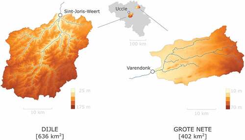
The study is conducted on two catchments in Belgium: the Dijle catchment upstream of Sint-Joris-Weert and the Grote Nete catchment upstream of Varendonk (Fig. 1). The Dijle catchment, located in the centre of Belgium, is dominated by sandy and loamy sand coverage. The Grote Nete catchment, located in the northeastern part of Belgium, has a predominantly sandy soil coverage, with parabolic land dunes present in the upstream parts. The main land uses for the Dijle and Grote Nete catchments include cropland (28% and 33%, respectively), grassland (15% and 19%), forest (31% and 23%) and urban and built-up area (19% and 19%). These catchments have been investigated in several previous climate change impact analyses (Vansteenkiste et al. 2012, 2014a, 2014b, Tavakoli et al. 2014, Van Hoey et al. 2014, Vrebos et al. 2014, Willems et al. 2014, Sunyer et al. 2015).

Figure 1. Selected catchments in Belgium.

For both catchments, lumped conceptual hydrological models NAM (Nielsen and Hansen 1973, DHI 2009), PDM (Moore 1985, 2007) and VHM (Willems 2014) are applied. The three hydrological models are forced with daily precipitation and ET_o data. Calibration is done using the optimization algorithm SCEM-UA (Vrugt et al. 2003), with a modified version of the Nash-Sutcliffe efficiency (NSE; Nash and Sutcliffe 1970) as objective function (Hartmann and Bárdossy 2005). With this modified version of NSE, the model is calibrated on different time scales simultaneously in order to enhance the performance of the conceptual hydrological models under changing conditions. Model evaluation is done by comparing observed and modelled streamflow series through performance indices such as NSE, RMSE-observation standard deviation ratio (RSR) and percent bias (PBIAS) (Moriasi et al. 2007). The performance of the three hydrological models after calibration is classified as satisfactory to good, with the exception of some performance indices of the NAM and PDM models for the Dijle catchment: NSE and RSR for the NAM model in the validation period and NSE and RSR for PDM in the calibration period (see Table 2 and Fig. 2).

Table 2. Hydrological signatures for the three hydrological models (NAM, PDM and VHM) calibrated for the Grote Nete and Dijle catchments. NSE: Nash-Sutcliffe efficiency (-); PBIAS (%): percent bias; and RSR: RMSE-observations standard deviation ratio (-).

	Grote Nete				Dijle
	NAM	PDM	VHM		NAM	PDM	VHM
Calibration period (22 May 2004–30 September 2009)
NSE	0.62	0.72	0.63	NSE	0.56	0.45	0.62
PBIAS	1.05	0.35	0.14	PBIAS	2.21	4.20	–0.33
RSR	0.59	0.53	0.61	RSR	0.66	0.74	0.62
Validation period (1 October 2009–1 October 2014)
NSE	0.57	0.56	0.55	NSE	0.48	0.50	0.54
PBIAS	–8.91	–16.9	–4.14	PBIAS	–18.8	–13.9	–1.34
RSR	0.65	0.66	0.67	RSR	0.72	0.70	0.68

Figure 2. Hydrographs for selected winter and summer events for both catchments.

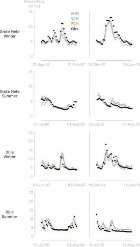
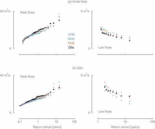
This study focuses particularly on peak flows and low flows, and therefore model performance evaluation is done for extreme events. Extreme flows are extracted from the time series using a peak-over-threshold (POT) method (Willems 2009). With this method, the time series are split into nearly independent events, based on multiple criteria such as peak height and minimum inter-event time. This allows peak- and low-flow values to be selected per event. The peak and low flows are ranked from more extreme to less extreme, and empirical return periods are assigned. This evaluation is visualized in Figure 3.

Figure 3. Evaluation of calibrated hydrological models for extreme peak and low flows for both catchments (2004–2014).

Current and projected hydro-meteorological time series

Observed precipitation and calculated ET_o data are available from measurements on a daily time step for the period 1901–2000 at the Uccle meteorological station (Fig. 1). The evapotranspiration is calculated following the Penman-Bultot method (Bultot et al. 1983), a modified Penman method (Penman 1948). This method uses mean sea-level pressure (psl), surface downwelling shortwave radiation (rsds), mean, maximum and minimum 2-m air temperature (tas, tasmax and tasmin, respectively), mean 10-m wind speed (sfcWind) and near-surface relative humidity (rhs) as input for the calculation of ET_o (see also Appendix A).

The total ensemble includes 20 global, CMIP5-based climate model runs, hereafter denoted as GCM runs, and comprises eight different models and four RCPs (RCP 2.6, 4.5, 6.0 and 8.5) (Table 3). For the selected climate model runs, data are available for precipitation and all meteorological variables required for the Penman-Bultot evapotranspiration calculation method. More information on the ET_o calculation method can be found in Baguis et al. (2010). The periods 1961–1990 and 2071–2100 are chosen as reference period and projection period, respectively.

Table 3. Selected global climate models.

Modelling centre or group	Institute ID	Model name	Emission scenario(s)
			RCP 8.5	RCP 6.0	RCP 4.5	RCP 2.6
College of Global Change and Earth System Science, Beijing Normal University	GCESS	BNU-ESM			×	×
Centre National de Recherches Météorologiques/Centre Européen de Recherche et Formation Avancée en Calcul Scientifique	CNRM -CERFACS	CNRM-CM5	×		×
NOAA Geophysical Fluid Dynamics Laboratory	NOAA GFDL	GFDL-ESM2G	×	×	×	×
		GFDL-ESM2M	×	×	×
Institute for Numerical Mathematics	INM	INM-CM4			×
Institut Pierre-Simon Laplace	IPSL	IPSL-CM5A-LR	×	×
		IPSL-CM5A-MR	×	×		×
Meteorological Research Institute	MRI	MRI-CGCM3	×		×	×

The projected time series for precipitation are obtained by applying an advanced perturbation method, accounting for the daily precipitation amount changes in a quantile-based way, and wet day frequency changes (Ntegeka et al. 2014). For ET_o, the delta change method is considered, where change factors are applied based on the mean evapotranspiration for reference and projection periods (Ntegeka et al. 2014).

Next, by comparing statistics for observed and projected time series, climate change signals are defined. Hydrological climate change impact analyses in Belgium are typically interested in winter peak flows and summer low flows. Therefore, relative changes in extreme daily (winter) precipitation amounts and duration of dry (summer) spells are analysed. A dry spell is defined as the total number of consecutive dry days, where precipitation on a dry day does not exceed 1 mm. After ranking variables such as daily precipitation, duration of dry spells and daily ET_o from extreme to less extreme, empirical return periods are assigned and empirical distributions are acquired. Per empirical return period, the relative change δ is calculated, expressed as a percentage:

(1) $\delta X\left(T\right)=\left(\frac{X{\left(T\right)}_{\mathrm{f}\mathrm{u}\mathrm{t}\mathrm{u}\mathrm{r}\mathrm{e}}-X{\left(T\right)}_{\mathrm{c}\mathrm{u}\mathrm{r}\mathrm{r}\mathrm{e}\mathrm{n}\mathrm{t}}}{X{\left(T\right)}_{\mathrm{c}\mathrm{u}\mathrm{r}\mathrm{r}\mathrm{e}\mathrm{n}\mathrm{t}}}\right)\times 100$(1)

where X is the variable of interest (daily precipitation, duration of dry spells and daily ET_o) and T the empirical return period. Changes can further be averaged over a range of return periods, if the behaviour of the changes is found to be stable within that range.

Note that the observed and projected time series have a length of 100 years, compared to the reference and projection periods, which are 30 years (1961–1990 and 2071–2100, respectively). The fact that length of the reference/projection periods is not equal to the length of the time series is handled by the advanced perturbation method of Ntegeka et al. (2014), by working in a quantile-based way.

Climate change impact assessment

Assuming stationarity of the hydrological model parameters, the hydrological models are forced by the current and projected time series. Next, characteristics of simulated rainfall–runoff time series are compared to quantify the impact of climate change on water resources. Extreme flows are extracted for current and projected time series based on a POT method (Willems 2009). After assigning empirical return periods for these extreme flows, changes are calculated per empirical return period according to Equation (1).

Uncoupling GCM variables

The set of available GCM runs results in 20 time series for precipitation and 20 time series of ET_o. Hydrological simulations are done for each possible combination of precipitation and ET_o. Simulations where the forcing data emerge from a single climate model run are labelled as “coupled” time series (20 in total). In contrast, the other possible combinations where forcing data for precipitation and ET_o emerge from different climate model runs are labelled as “uncoupled” time series (20 × 19 = 380 in total).

The impact of the uncoupling can now be evaluated by comparing the coupled and uncoupled time series through:

• hydrological signatures: NSE, PBIAS and RSR (see above);

• empirical cumulative distributions for both peak and low flows and corresponding impact factors.

Results

Precipitation and ET_o climate change signals

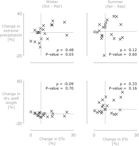
An overview of the precipitation and ET_o climate change signals is presented in Figure 4, with Figures 5 and 6 presenting the changes in the periods 1961–1990 and 2071–2100. Changes in daily precipitation amounts and frequency are considered, as well as changes in monthly ET_o amounts.

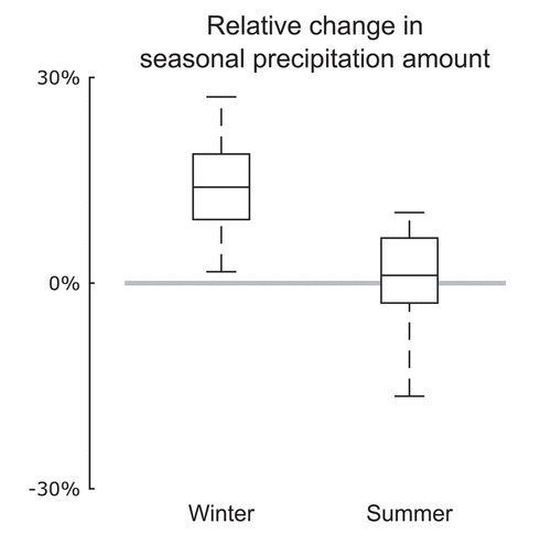
Extreme daily precipitation amounts (Fig. 4(a)) are very likely to increase for both seasons, as 18 (winter) and 19 (summer) of the 20 GCM runs predict, on average, positive changes. For return periods up to 10–30 years, changes remain constant: changes vary in the range [–8%, +32%] in winter and [–20%, +41%] in summer. Furthermore, for more extreme events, both the median change and variance increase with increasing return period. For the 100-year empirical return period, winter changes vary in the range [0%, +85%], and summer changes in the range [–30%, +160%]. The average seasonal precipitation amount is expected to increase in winter (October–March), since all GCM runs predict positive changes (Fig. 5); for summer (April–September), the various GCM runs do not show any agreement on the sign of the change (Fig. 5).

Figure 4. Climate change signals for both catchments for (a) daily precipitation amounts (relative changes for empirical return periods, per season), (b) dry spell durations (relative changes for empirical return periods, per season) and (c) average monthly evapotranspiration amount (absolute mean monthly values). Reference period 1961–1990; projection period 2071–2100.

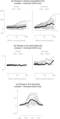
Figure 5. Relative changes for both catchments in seasonal precipitation amount for winter and summer periods. Reference period 1961–1990; projection period 2071–2100.

It is likely that the duration of dry spells will increase in summer, as 14 of the 20 GCM runs predict positive changes, irrespective of return period (Fig. 4(b)). However, the magnitude of these changes is poorly known: e.g. the duration of a dry spell in summer with a 10-year empirical return period will change in the range [–5%, +45%] (Fig. 4(b)). In contrast, for winter, the GCM results are not in agreement with respect to dry-spell lengths; however, changes are projected to be small [–15%, +10%] (Fig. 4(b)). Finally, the number of wet days is virtually certain to increase in winter and likely to decrease in summer (Fig. 6).

Figure 6. Relative changes for both catchments in wet day frequency for winter and summer periods. Reference period 1961–1990; projection period 2071–2100.

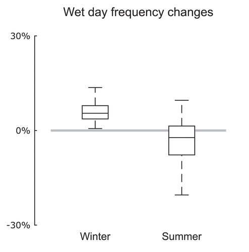
Figure 7. Relative frequency of peak flow events per month. Thick black line represents current conditions, grey lines represent the considered climate model runs for the projection period 2071–2100.

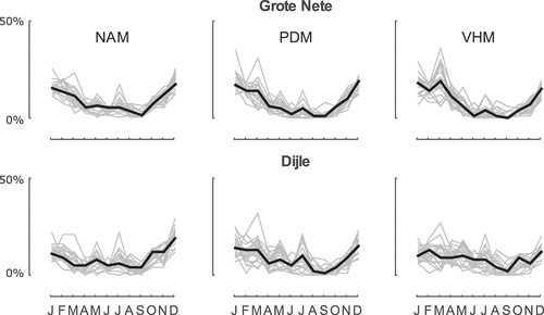
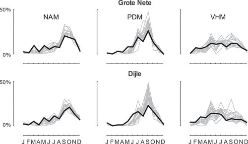
Figure 8. Relative frequency of low flow events per month. Thick black line represents current conditions, grey lines represent the considered climate model runs for the projection period 2071–2100.

The climate change signals for the average monthly ET_o amount are shown in Figure 4(c). Firstly, a seasonal dependence is observed, where the summer changes are typically stronger than the winter changes. For January (Jan) and July (Jul), a typical winter and summer month, respectively, the changes are in the ranges [0.00 mm/d, +0.10 mm/d] and [–0.05 mm/d, +0.85 mm/d], respectively (Fig. 4(c)). Furthermore, based on these GCM runs, it is very likely that the ET_o amount will increase for all months by the end of the 21st century.

Correlation in climate change signals

For the catchments considered, extreme peak flows typically relate to extreme daily winter precipitation amounts and mostly occur in the middle of winter periods (Fig. 7). In turn, extreme low flows originate from long dry summer spells and occur towards the end of summer (Fig. 8). In this context, Figure 9 shows the correlation between the change in the average seasonal ET_o amount and the change in extreme daily precipitation amount (top panels) or dry-spell durations (bottom panels). The Pearson correlation coefficients were calculated with corresponding P values (Fig. 9). A P value less than 0.05 indicates a correlation significantly different from zero at the 95% confidence level. For the considered climate model ensemble, and for these catchments, a (positive) correlation between the winter ET_o and precipitation changes appears. However, for the summer season, no significant correlation is found; nor are the ET_o changes correlated with the dry-spell duration changes, based on the selected criteria. Note that the data points in Figure 9 are based on the average climate change signals for empirical return periods between 1 and 30 years.

Figure 9. Climate change signals (relative changes) for both catchments for average seasonal ET_o amount versus extreme daily precipitation amount (top) and dry spell duration (bottom). Crosses indicate the results for the coupled climate model runs; grey lines indicate median results. Correlation coefficients ρ and corresponding P values indicate possible correlation between the variables.

Effect of uncoupling the GCM variables

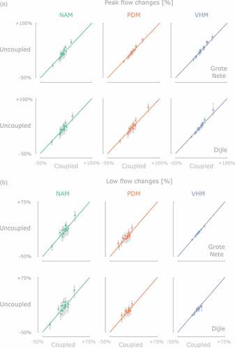
The effects of uncoupling the precipitation and ET_o climate change signals are shown in Figures 10 and 11. Hydrological signatures (NSE, PBIAS and RSR), shown in Figure 10, indicate good to very good performance of rainfall–runoff series based on uncoupled ensemble members compared to rainfall–runoff series of the coupled ensemble member, based on the criteria of Moriasi et al. (2007). For calculation of the hydrological signatures, the coupled ensemble member was taken as the “observed series”, whereas the uncoupled member was taken as the “modelled series”. Furthermore, Figure 11 shows relative changes of future extreme peak (and low) flows based on uncoupled ensemble members versus coupled ensemble members. The maximum bias introduced by replacing the coupled ET_o changes by ET_o changes of another GCM run is 17% for peak flows and 20% for low flows. Average values, however, are limited to 0.07% and 0.05%, respectively.

Figure 10. Hydrological signatures for the uncoupled streamflow series compared with the coupled series. Circles represent the median result, black horizontal lines represent the full spread of results. NSE: Nash-Sutcliffe efficiency; PBIAS: percent bias; and RSR: RMSE-observations standard deviation ratio. Performance ratings (unsatisfactory to very good) taken from Moriasi et al. (2007).

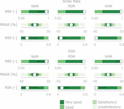
Figure 11. Changes for coupled vs uncoupled ensemble members, for peak flows and low flows, for both catchments and three hydrological models. Coloured dots indicate median values.

Discussion and conclusions

Towards the end of the 21st century, wetter winters, i.e. increasing winter precipitation amount, and drier summers, i.e. decreasing summer precipitation amount, are projected for Belgium (Tabari et al. 2015, Hosseinzadehtalaei et al. 2017a) and western Europe in general (Jacob et al. 2014, KNMI 2015). This is generally in agreement with the results of the present study. Previous studies show a decreasing summer precipitation, whereas our results are inconclusive. This is mainly due to the selected ensemble of climate model runs. We could use only climate model runs delivering all the necessary variables for calculation of ET_o according to Penman-Bultot (mean sea-level pressure, total radiation balance, temperature, wind speed and humidity).

A weak correlation was found within climate models between the change signals for extreme daily precipitation and ET_o amounts in winter. However, this correlation appears less important after propagation of the meteorological series in the hydrological impact model and is damped out throughout the impact modelling chain. No significant bias was found for peak flow impacts when randomly replacing the climate model used for deriving ET_o changes: the average bias for peak flow is equal to 0.07%, which is considered insignificant. Regarding low flows, mainly caused by long dry spells in summer periods, no correlation was found between dry spell duration changes and ET_o changes. As expected, on average, impact results for low flows do not show any significant bias when randomly replacing the climate model used for deriving ET_o changes: the average bias for low flow change is as small as 0.05%.

Previous research also reported on the correlation between relative changes in precipitation and relative changes in ET_o for the same area. Tabari et al. (2015) found “… no strong relationship for both winter and summer seasons”. In the first instance, this seems to contradict our results. However, it must be noted that they used the mean monthly change in precipitation, whereas here the change in extreme precipitation and changes in dry spell lengths are considered. Moreover, Tabari et al. (2015) considered four seasons of three months per year, whereas here six-month seasons are applied. In another study with different research objectives, Ntegeka et al. (2014) also looked into the correlation of changes in precipitation and ET_o amounts. They applied the same method for deriving the climate change signals, based on a set of 28 regional climate models, and with four seasons of three months per year. The results obtained by Ntegeka et al. (2014) are comparable with our study. Furthermore, our results are consistent with those of Adler et al. (2008), who investigated the relationship between anomalies in precipitation and surface temperature on a global scale. The surface temperature could serve as a proxy for ET_o, as this is one of the most important drivers of ET_o.

On average, no significant bias was seen by uncoupling the climate change signals for precipitation and ET_o. We acknowledge that bias may have been introduced for some individual combinations. However, when ensembles of climate change signals were considered, and after propagation in the hydrological models, these became insignificant. Moreover, for both peak and low flows, the biases remained smaller than the differences between the median impacts of coupled ensemble members for the different hydrological models. Finally, when considering the median of all uncoupled results, the minor biases were reduced even more.

This study used only 20 climate model runs for precipitation. However, for the case studies considered, 160 climate model runs are available for precipitation within the CMIP5 ensemble. Only for the 20 selected runs, ET_o can be calculated based on a combinational method, e.g. Penman-based. Traditionally, one would only include 20 climate model runs in an ensemble for (hydrological) impact modelling. We have shown that, for our case study, it is possible to include all 160 available climate model runs for precipitation (i.e. 20 runs where the corresponding ET_o calculation is possible and 140 runs where it is not). The disadvantage, however, is that such an ensemble requires a significant amount of simulations: per combination of hydrological model and catchment, one ends up with 2820 simulations (i.e. 140 P-GCM runs × 20 ET_o-GCM runs + 20 P-GCM runs × 1 ET_o-GCM run). This might present a challenge in computational time and one needs to be very cautious and conscientious when interpreting results and drawing conclusions from this big dataset. The computational disadvantage, though, is not considered as a problem for impact calculations on river hydrology, since ample conceptual models exist that require little calculation time. In our case, we performed 2400 simulations (20 P-GCM runs × 20 ET_o-GCM runs × 3 hydrological models × 2 catchments), which took 680 seconds in Matlab 2014b, run on a PC with MS Windows 10 (64 bit), i7 2.70 GHz processor and 8.00 GB RAM. In turn, for urban applications and for distributed models where computational requirements are often very high, this might be an important limitation.

Acknowledgements

We acknowledge the World Climate Research Programme’s Working Group on Coupled Modelling, which is responsible for CMIP, and thank the climate modelling groups for producing and making available their model output. Finally, Hossein Tabari is acknowledged for calculating the evapotranspiration for the climate model data. This was completed in a previous study. The climate model data are available through the website of the Earth System Grid Federation, https://esgf.llnl.gov/. The meteorological observations at Uccle were made available by the Royal Meteorological Institute of Belgium.

Disclosure statement

No potential conflict of interest was reported by the authors.

Additional information

Funding

The second author obtained a scholarship from the Fund for Scientific Research (FWO) - Flanders. This financial support is gratefully acknowledged.

Appendix A. The Penman-Bultot method for potential evapotranspiration

The evaporation of a free water surface is computed as:

(A1) $E_0=\frac{\delta Q_0^{\ast }/L+\gamma \left(\alpha +\beta u\right)\left(\epsilon -e\right)}{\gamma \mathit{+}\delta }$(A1)

with

(A2) $\delta ={\left(\frac{d\epsilon }{dT}\right)}_T$(A2)

(A3) $Q_0^{\ast }=\left(1-{\alpha }_0\right)K_s-L^{\ast }$(A3)

(A4) $\gamma \mathit{=}0.000662p$(A4)

where $Q_0^{\ast }$ is the total radiation balance; $K_s$is the global solar radiation; ${\alpha }_0$is the free water surface albedo; $L^{\ast }$is net terrestrial radiation; $L$ is the latent heat of vaporization of water; $\gamma$ is a psychrometric coefficient; $p$ is mean annual atmospheric pressure; $u$ is mean daily wind speed; $\epsilon -e$ is the saturation deficit; and $\alpha$ and $\beta$ are location-specific parameters, determined with evaporation measurements known for 11 Belgian locations (Bultot et al. 1983). Here, $\alpha =0.205$ and $\beta =0.028$.

The free water surface albedo is calculated using:

(A5) ${\alpha }_0=0.07+\left(A-0.07\right)I{r}^{0.4}$(A5)

where A is the albedo of the free water surface under a clear sky (tabulated as a function of month of the year and Ir), and Ir is the relative insolation.

Net terrestrial radiation, $L^{\ast }$, is calculated as:

(A6) $L^{\ast }=\sigma T^4\left(1-\left(a+b\sqrt{e}\right)\left(1+c{\left(1-Ir\right)}^2\right)\right)$(A6)

where $\sigma$ is the Stefan-Boltzmann constant, $e$ is the water vapour pressure and $T$ is the air temperature. Parameters a, b and c can be determined by measurements of radiation variables, and are location specific. Bultot et al. (1983) determined seasonal values for the station at Uccle.

Based on a ratio involving $a_i$ (the albedo of a natural cover surface), one is able to transfer the above evaporation of a free water surface E₀ to the potential evapotranspiration of a natural cover EToi.

References

- Adler, R.F., et al., 2008. Relationships between global precipitation and surface temperature on interannual and longer timescales (1979–2006). Journal of Geophysical Research, 113, D22104. doi:10.1029/2008JD010536
- Baguis, P., et al., 2010. Climate change scenarios for precipitation and potential evapotranspiration over central Belgium. Theoretical and Applied Climatology, 99, 273–286. doi:10.1007/s00704-009-0146-5
- Birkinshaw, S.J., et al., 2017. Climate change impacts on Yangtze River discharge at the Three Gorges Dam. Hydrology and Earth System Sciences, 21, 1911–1927. doi:10.5194/hess-21-1911-2017
- Bultot, F., Coppens, A., and Dupriez, G.L., 1983. Estimation de l’évapotranspiration potentielle en Belgique (Procédure Révisée). Uccle - Brussels, Belgium: Institut Royal Météorologique.
- Bürger, G., et al., 2013. Downscaling extremes: an intercomparison of multiple methods for future climate. Journal of Climate, 26, 3429–3449. doi:10.1175/JCLI-D-12-00249.1
- Ceola, S., et al., 2015. Virtual laboratories: new opportunities for collaborative water science. Hydrology and Earth System Sciences, 19, 2101–2117. doi:10.5194/hess-19-2101-2015
- Chamorro, A., et al., 2017. Effect of (quasi-) optimum model parameter sets and model characteristics on future discharge projection of two basins from Europe and Asia. Climatic Change, 142, 559–573. doi:10.1007/s10584-017-1974-4
- Chen, J., et al., 2011. Overall uncertainty study of the hydrological impacts of climate change for a Canadian watershed. Water Resources Research, 47, 1–16. doi:10.1029/2011WR010602
- Dams, J., et al., 2015. Multi-model approach to assess the impact of climate change on runoff. Journal of Hydrology, 529, 1601–1616. doi:10.1016/j.jhydrol.2015.08.023
- de Boer-Euser, T., et al., 2017. Looking beyond general metrics for model comparison - lessons from an international model intercomparison study. Hydrology and Earth System Sciences, 21, 423–440. doi:10.5194/hess-21-423-2017
- DHI (Danish Hydrological Institute) (2009) Mike 11 software manual. Available form: https://www.mikepoweredbydhi.com/products/mike-11 [14 Mar 2015]
- Drouet, L., Bosetti, V., and Tavoni, M., 2015. Selection of climate policies under the uncertainties in the fifth assessment report of the IPCC. Nature Climate Change, 5, 937–940. doi:10.1038/nclimate2721
- Ekström, M., et al., 2016. The method of producing climate change datasets impacts the resulting policy guidance and chance of mal-adaptation. Climate Services, 4, 13–29. doi:10.1016/J.CLISER.2016.09.003
- Ekström, M., Grose, M.R., and Whetton, P.H., 2015. An appraisal of downscaling methods used in climate change research. WIREs Climate Change, 6, 301–319. doi:10.1002/wcc.339
- Fatichi, S., et al., 2016. Uncertainty partition challenges the predictability of vital details of climate change. Earth’s Future, 4, 240–251. doi:10.1002/2015EF000336
- Fowler, H.J., Blenkinsop, S., and Tebaldi, C., 2007. Linking climate change modelling to impacts studies: recent advances in downscaling techniques for hydrological modelling. International Journal of Climatology, 27, 1547–1578. doi:10.1002/joc.1556
- Gosling, S.N., et al., 2017. A comparison of changes in river runoff from multiple global and catchment-scale hydrological models under global warming scenarios of 1°C, 2°C and 3°C. Climatic Change, 141, 577–595. doi:10.1007/s10584-016-1773-3
- Habets, F., et al., 2013. Impact of climate change on the hydrogeology of two basins in northern France. Climatic Change, 121, 771–785. doi:10.1007/s10584-013-0934-x
- Hartmann, G. and Bárdossy, A., 2005. Investigation of the transferability of hydrological models and a method to improve model calibration. Advances in Geoscience, 5, 83–87. doi:10.5194/adgeo-5-83-2005
- Hawkins, E. and Sutton, R., 2009. The potential to narrow uncertainty in regional climate predictions. Bulletin of the American Geological Society, 90, 1095–1107. doi:10.1175/2009BAMS2607.1
- Hosseinzadehtalaei, P., Tabari, H., and Willems, P., 2017a. Uncertainty assessment for climate change impact on intense precipitation : how many model runs do we need? International Journal of Climatology, 37, 1105–1117. doi:10.1002/joc.5069
- Hosseinzadehtalaei, P., Tabari, H., and Willems, P., 2017b. Quantification of uncertainty in reference evapotranspiration climate change signals in Belgium. Hydrology Research, 48, 1391–1401. doi:10.2166/nh.2016.243
- Hundecha, Y., et al., 2016. Inter-comparison of statistical downscaling methods for projection of extreme flow indices across Europe. Journal of Hydrology, 541, 1273–1286. doi:10.1016/j.jhydrol.2016.08.033
- Islam, S.U., Dery, S.J., and Werner, A.T., 2017. Future climate change impacts on snow and water resources of the Fraser River Basin, British Columbia. Journal of Hydrometeorology, 18, 473–496. doi:10.1175/JHM-D-16-0012.1
- Jacob, D., et al., 2014. EURO-CORDEX: new high-resolution climate change projections for European impact research. Regional Environmental Change, 14, 563–578. doi:10.1007/s10113-013-0499-2
- Katz, R.W., et al., 2013. Uncertainty analysis in climate change assessments. Nature Climate Change, 3, 769–771. doi:10.1038/nclimate1980
- Kingston, D.G., et al., 2009. Uncertainty in the estimation of potential evapotranspiration under climate change. Geophysical Research Letters, 36, 3–8. doi:10.1029/2009GL040267
- KNMI (Koninklijk Nederlands Meteorologisch Instituut), 2015. KNMI’14 climate scenarios for the Netherlands; A guide for professionals in climate adaptation. De Bilt, The Netherlands.
- Koch, J., et al., 2016. Inter-comparison of three distributed hydrological models with respect to seasonal variability of soil moisture patterns at a small forested catchment. Journal of Hydrology, 533, 234–249. doi:10.1016/J.JHYDROL.2015.12.002
- Kunreuther, H., et al., 2014. Integrated risk and uncertainty assessment of climate change response policies coordinating lead authors: integrated risk and uncertainty assessment of climate change response policies. In: O. Edenhofer, et al., eds. Climate change 2014: mitigation of climate change. Contribution of working group III to the fifth assessment report of the intergovernmental panel on climate change. Cambridge, UK: Cambridge University Press, 151–205.
- Liu, J., et al., 2017. Local climate change and the impacts on hydrological processes in an arid alpine catchment in Karakoram. Water, 9, 1–17. doi:10.3390/w9050344
- Liu, T., et al., 2011. Climate change impact on water resource extremes in a headwater region of the Tarim basin in China. Hydrology and Earth System Sciences, 15, 3511–3527. doi:10.5194/hess-15-3511-2011
- Maraun, D., 2016. Bias correcting climate change simulations - a critical review. Current Climate Change Reports, 2, 211–220. doi:10.1007/s40641-016-0050-x
- Maraun, D., et al., 2010. Precipitation downscaling under climate change: recent developments to bridge the gap between dynamical models and the end user. Reviews of Geophysics, 48 (3). doi:10.1029/2009RG000314
- McMillan, H., et al., 2017. How uncertainty analysis of streamflow data can reduce costs and promote robust decisions in water management applications. Water Resources Research, 53, 5220–5228. doi:10.1002/2016WR020328
- Meaurio, M., et al., 2017. Assessing the hydrological response from an ensemble of CMIP5 climate projections in the transition zone of the Atlantic region (Bay of Biscay). Journal of Hydrology, 548, 46–62. doi:10.1016/j.jhydrol.2017.02.029
- Milly, P.C.D. and Dunne, K.A., 2016. Potential evapotranspiration and continental drying. Nature Climate Change, 6, 946–949. doi:10.1038/nclimate3046
- Milly, P.C.D. and Dunne, K.A., 2017. A hydrologic drying bias in water-resource impact analyses of anthropogenic climate change. Journal of the American Water Resources Assocication JAWRA, 53, 822–838. doi:10.1111/1752-1688.12538
- Monteith, J.L., 1965. Evaporation and the environment. In: The state and movement of water in living organisms, XIXth symposium, Swansea UK. Cambridge, UK: Cambridge University Press, pp 205–234.
- Moore, R.J., 1985. The probability-distributed principle and runoff production at point and basin scales. Hydrological Sciences Journal, 30, 273–297. doi:10.1080/02626668509490989
- Moore, R.J., 2007. The PDM rainfall–runoff model. Hydrology and Earth System Sciences, 11, 483–499. doi:10.5194/hess-11-483-2007
- Moriasi, D.N., et al., 2007. Model evaluation guidelines for systematic quantification of accuracy in watershed simulations. Transactions of the American Society for Agricultural and Biological Engineering (ASABE), 50, 885–900.
- Moss, R.H., et al., 2010. The next generation of scenarios for climate change research and assessment. Nature, 463, 747–756. doi:10.1038/nature08823
- Nash, J.E. and Sutcliffe, J.V., 1970. River flow forecasting through conceptual models part I: A discussion of principles. Journal of Hydrology, 10, 282–290. doi:10.1016/0022-1694(70)90255-6
- Nicolle, P., et al., 2014. Benchmarking hydrological models for low-flow simulation and forecasting on French catchments. Hydrology and Earth System Sciences, 18, 2829–2857. doi:10.5194/hess-18-2829-2014
- Nielsen, S.A. and Hansen, E., 1973. Numerical simulation of the rainfall-runoff process on a daily basis. Nordic Hydrology, 4, 171–190. doi:10.2166/nh.1973.0013
- Ntegeka, V., et al., 2014. Developing tailored climate change scenarios for hydrological impact assessments. Journal of Hydrology, 508, 307–321. doi:10.1016/j.jhydrol.2013.11.001
- Paparrizos, S., Maris, F., and Matzarakis, A., 2017. Sensitivity analysis and comparison of various potential evapotranspiration formulae for selected Greek areas with different climate conditions. Theoretical and Applied Climatology, 128 (3–4), 745–759. doi:10.1007/s00704-015-1728-z
- Patt, A.G. and Weber, E.U., 2014. Perceptions and communication strategies for the many uncertainties relevant for climate policy. WIREs Climate Change, 5, 219–232. doi:10.1002/wcc.259
- Penman, H.L., 1948. Natural evaporation from open water, bare soil and grass. Proceedings of the Royal Society London A, Mathematical, Physical and Engineering Sciences, 193, 120–145.
- Reshmidevi, T.V., et al., 2017. Estimation of the climate change impact on a catchment water balance using an ensemble of GCMs. Journal of Hydrology. doi:10.1016/j.jhydrol.2017.02.016
- Seiller, G. and Anctil, F., 2016. How do potential evapotranspiration formulas influence hydrological projections? Hydrological Sciences Journal, 61, 2249–2266. doi:10.1080/02626667.2015.1100302
- Seiller, G., Roy, R., and Anctil, F., 2017. Influence of three common calibration metrics on the diagnosis of climate change impacts on water resources. Journal of Hydrology, 547, 280–295. doi:10.1016/j.jhydrol.2017.02.004
- Seong, C., Sridhar, V., and Billah, M.M., 2017. Implications of potential evapotranspiration methods for streamflow estimations under changing climatic conditions. International Journal of Climatology. doi:10.1002/joc.5218
- Sunyer, M.A., et al., 2015. Inter-comparison of statistical downscaling methods for projection of extreme precipitation in Europe. Hydrology and Earth System Sciences, 19, 1827–1847. doi:10.5194/hess-19-1827-2015
- Tabari, H., Taye, M.T., and Willems, P., 2015. Water availability change in central Belgium for the late 21st century. Global Planetary Change, 131, 115–123. doi:10.1016/j.gloplacha.2015.05.012
- Tavakoli, M., et al., 2014. Impact of climate change and urban development on extreme flows in the Grote Nete watershed, Belgium. Natural Hazards, 71, 2127–2142. doi:10.1007/s11069-013-1001-7
- Taylor, K.E., Stouffer, R.J., and Meehl, G.A., 2012. An overview of CMIP5 and the experiment design. Bulletin of the American Geological Society, 93, 485–498. doi:10.1175/BAMS-D-11-00094.1
- Teklesadik, A.D., et al., 2017. Inter-model comparison of hydrological impacts of climate change on the Upper Blue Nile basin using ensemble of hydrological models and global climate models. Climatic Change, 141, 517–532. doi:10.1007/s10584-017-1913-4
- Teng, J., et al., 2011. Estimating the relative uncertainties sourced from gcms and hydrological models in modeling climate change impact on runoff. Journal of Hydrometeorology, 13, 122–139. doi:10.1175/JHM-D-11-058.1
- Teshager, A.D., et al., 2016. Assessment of impacts of agricultural and climate change scenarios on watershed water quantity and quality, and crop production. Hydrology and Earth System Sciences, 20, 3325–3342. doi:10.5194/hess-20-3325-2016
- Thornthwaite, C.W. and Mather, J.R., 1951. The role of evapotranspiration in climate. Archiv für Meteorologie Geophysik und Bioklimatologie Serie B, 3, 16–39. doi:10.1007/BF02242588
- Van Hoey, S., et al., 2014. A qualitative model structure sensitivity analysis method to support model selection. Journal of Hydrology, 519, 3426–3435. doi:10.1016/j.jhydrol.2014.09.052
- Van Uytven, E. and Willems, P., 2018. Greenhouse gas scenario sensitivity and uncertainties in precipitation projections for central Belgium. Journal of Hydrology, 558, 9–19. doi:10.1016/j.jhydrol.2018.01.018
- van Vuuren, D.P., et al., 2011. The representative concentration pathways: an overview. Climatic Change, 109, 5–31. doi:10.1007/s10584-011-0148-z
- Vansteenkiste, T., et al., 2012. Climate change impact on river flows and catchment hydrology: A comparison of two spatially distributed models. Hydrological Processes, 3662, 3649–3662. doi:10.1002/hyp.9480
- Vansteenkiste, T., et al., 2014a. Intercomparison of hydrological model structures and calibration approaches in climate scenario impact projections. Journal of Hydrology, 519, 743–755. doi:10.1016/j.jhydrol.2014.07.062
- Vansteenkiste, T., et al., 2014b. Intercomparison of five lumped and distributed models for catchment runoff and extreme flow simulation. Journal of Hydrology, 511, 335–349. doi:10.1016/j.jhydrol.2014.01.050
- Vrebos, D., et al., 2014. Water displacement by sewer infrastructure in the Grote Nete catchment, Belgium, and its hydrological regime effects. Hydrology and Earth System Sciences, 18, 1119–1136. doi:10.5194/hess-18-1119-2014
- Vrugt, J.A., et al., 2003. A shuffled complex evolution metropolis algorithm for optimization and uncertainty assessment of hydrologic model parameters. Water Resources Research, 39. doi:10.1029/2002WR001642
- Willems, P., 2009. A time series tool to support the multi-criteria performance evaluation of rainfall-runoff models. Environmental Modelling and Software, 24, 311–321. doi:10.1016/j.envsoft.2008.09.005
- Willems, P., 2014. Parsimonious rainfall-runoff model construction supported by time series processing and validation of hydrological extremes - Part 1: step-wise model-structure identification and calibration approach. Journal of Hydrology, 510, 578–590. doi:10.1016/j.jhydrol.2014.01.017
- Willems, P., et al., 2014. Parsimonious rainfall-runoff model construction supported by time series processing and validation of hydrological extremes - Part 2: intercomparison of models and calibration approaches. Journal of Hydrology, 510, 591–609. doi:10.1016/j.jhydrol.2014.01.028