Parameter identification in hydrological models using groundwater-level measurements and satellite-based soil moisture

ABSTRACT

The main objective was to identify representative parameter sets for two mesoscale catchments. Discharge, groundwater level and satellite-based soil moisture were included in the calibration process to increase the robustness and the representativeness of the parameters. The integration of these data led to an innovative, detailed soil water description, which was implemented in a hydrological model with its corresponding parameters as an appropriate interface to optimization algorithms. A new lexicographic calibration strategy was applied. A comparison with results obtained by the SCE-UA (shuffled complex evolution algorithm) optimization showed that the lexicographic approach delivered more similar parameter sets, had more similar effects on the hydrological system and was much faster. The similarity of the parameter values and the cross-validation scores indicates the good representativeness of the model and furthermore emphasizes the application of a lexicographic calibration procedure. The consideration of groundwater level was a clear-cut benefit for the calibration, while the consideration of satellite-based soil moisture showed no significant effects in the two catchments.

KEYWORDS:

• hydrological modelling
• soil water simulation
• multi-objective calibration
• optimization
• lexicographic approach

Editor S. Archfield Associate editor N. Verhoest

1 Introduction

The demands on hydrological models have increased since the performance of computers has been improved. Common tasks for hydrological models include planning applications, operational tasks, such as flood forecasting, or scientific questions. To meet all these requirements, the development, improvement and parameter estimation of hydrological models have been strongly prioritized in hydrology. In the study at hand, we focus on a new multi-objective lexicographic calibration strategy to identify representative parameters for two selected catchments.

The complexity of modern hydrological model systems requires effective calibration techniques in order to find representative model parameters for the simulated hydrological regime. In the past 10 years, the calibration methods have shifted from single-criterion towards multi-criteria and multi-objective techniques (Efstratiadis and Koutsoyiannis 2010). Essential aspects in parameter identification, besides the goodness of fit in calibration/validation, are the transferability and plausibility of the calibration parameters as well as the time efficiency of the calibration procedure. Further, a model needs to provide appropriate process-related interfaces that allow calibration on multi-objective variables. For usage of measurements of satellite-based soil moisture within the calibration process, for instance, the soil model has to be designed in such a way that simulated water content for the upper 5 cm is individually evaluated and can be accessed as a calibration interface.

Hydrological model applications require various data for the structural model set-up. This includes, for example, topographic information, land-use information and soil maps. Time series data such as rainfall or discharge are needed as primary boundary conditions and for the calibration of the model. Due to technical difficulties in measuring these data, they often introduce uncertainties, gaps or other implausibilities. For this reason, hydrologists tend to use robust calibration methods to avoid influences of measurement errors (Bárdossy and Singh 2008). Numerous applications in modelling work with long-term simulations, which are needed, for example, in extreme value statistics or climate impact research (Schewe et al. 2014, Al-Safi and Sarukkalige 2017, Hattermann et al. 2017). To achieve credible results in this context, calibration parameters need to be representative and reliable beyond the calibration period (Merz et al. 2011). Further, the calculation time of process-based hydrological models can be high, in particular for applications on large catchments (Zhang et al. 2009). In this context, optimization strategies are required that reliably identify plausible calibration parameter sets with few iteration steps (Gelleszun et al. 2017).

In various published studies, different types of data have been used in the calibration of hydrological models. Sutanudjaja et al. (2014) presented a stepwise calibration of a large-scale coupled groundwater–land surface model (see also Sutanudjaja et al. 2018 for the improved version). They performed more than 3000 simulation runs and retrospectively evaluated quality criteria of simulated values for discharge, soil moisture and groundwater-level time series versus observed ones. The soil moisture observation was based on the soil water index (SWI) derived from the European remote sensing scatterometer. The SWI is an empirical value calculated from satellite-based measurements for the upper soil layer (few centimetres) by applying a low-pass filter (Wagner et al. 1999b). The cumulative distribution function (cdf) of the simulated soil water content was scaled to match the cdf of the SWI. After that, the mean absolute error (MAE) was used as the objective function to compare simulated and observed soil moisture. They concluded that the SWI is suitable for calibrating soil moisture in low-lying areas. López López et al. (2016) used a Kalman filter to assimilate data from the AMSR-E¹ into the global hydrological model PCR-GLOBWB (Van Beek and Bierkens 2008). The root mean square error (RMSE) was used as the objective function to compare simulated and observed soil moisture. They concluded that the assimilation of soil moisture observations yields significant improvements in the model estimates of discharge. Laiolo et al. (2016) improved the calibration results of discharge in a small catchment by including satellite-based soil moisture in the calibration. Crow et al. (2017) improved flow forecasts by integrating satellite-based soil moisture into the initial soil water conditions. Wanders et al. (2014) used satellite-based soil moisture data of AMSR-E, ASCAT² and SMOS³ to investigate if these data improve the calibration of the hydrological model LISFLOOD (van der Knijff et al. 2010) and which calibration parameters are affected. The RMSE was used as the objective function to compare simulated and observed soil moisture. They concluded that remotely sensed soil moisture improves the calibration of the hydrological model in small catchments.

In general, various challenges emerge when dealing with multi-objective calibration. On the one hand, there is often an imbalance between model resolution and data scale. Penetration depth of satellite-based measurements of soil moisture, for example, is only a few centimetres at commonly used C-band frequencies (see e.g. Albergel et al. 2010, 2009). In contrast, soil storages in models struggle with numerical stability if they are too small. Further, groundwater levels are usually not simulated in meso- or large-scale hydrological models, since these models are designed to simulate the catchment discharge. Groundwater models, on the other hand, require detailed data about the underground structure (geology) and require huge computational effort. Another challenge in hydrological modelling is the identification of representative and robust calibration parameter sets (Gelleszun et al. 2017). Optimization approaches are often controlled by mathematical rules. In this context, excellent calibration results may face problems in validation. Manual calibration, on the other hand, is subjective and therefore not reproducible by others. Further, objective functions have to be set with respect to the affected variables. It is, for example, questionable to apply absolute criteria such as the RMSE on soil moisture comparisons because of a possible bias in absolute values retrieved by satellite data (see e.g. Drusch et al. 2004, Löw et al. 2007, Pathe et al. 2009 or Liu et al. 2011). Another challenge is the large computation time of process-based distributed hydrological models combined with multi-objective optimization algorithms. The computation time of large-scale models can be extensive (up to several days for a single simulation run). For this reason, optimization strategies are required that generate reliable results with few iterations. In addition, an a priori consideration of the preferences for the multi-objective optimization task leads to fewer iteration steps.

Accordingly, the objectives of this study are:

• Presentation of an innovative soil water model suited for meso- and macroscale hydrological model applications.

• Extension of the lexicographic strategy based on Gelleszun et al. (2017) by including the multi-objective observations of discharge (Q), groundwater level (GW) and soil moisture (θ).

• Application of the hydrological model with the extended lexicographic calibration strategy on two mesoscale catchments in northern Germany.

In this context, we present a newly developed, innovative soil water model, which is implemented in the hydrological modelling system PANTA RHEI (see Section 2.1). The model has an interface to apply a lexicographic calibration strategy (Gelleszun et al. 2017), which we extended by involving multi-objective observations. The soil water model provides the needed interfaces for multi-objective calibration (subgrid simulations for soil moisture and approximation of groundwater level). The fundamental idea of the lexicographic calibration strategy is to determine an order of preference of objective functions prior to the calibration. This order is dependent on the scientific context, the focus of the project and the available data. The grouping of parameters and the sequential procedure allows the integration of different objective functions and thus reduces the search space with the advantage of saving calculation time. Analyses of parameter reliability and the impact of the parameters on model results were conducted via cross-validation and comparison of the results with those obtained by the commonly used optimization algorithm SCE-UA⁴ (Duan et al. 1992). Following Duan et al. (1992, 1993), the SCE global optimization algorithm combines the downhill-simplex procedure (Nelder and Mead 1965) with concepts of controlled random search (Price 1987), competitive evolution (Holland 1975) and complex shuffling.

2 Methodology

2.1 Hydrological model PANTA RHEI

PANTA RHEI is a deterministic, semi-distributed, physically-based hydrological model for long-term or single-event simulations. It provides an API⁵ to apply individual optimization methods. The PANTA RHEI model was developed by the Department of Hydrology, Water Management and Water Protection, Leichtweiss Institute for Hydraulic Engineering and Water Resources, University of Braunschweig, in co-operation with the Institut für Wassermanagement IfW GmbH, Braunschweig (LWI-HYWAG und IfW 2012). It has been successfully applied for scientific questions (Hölscher et al. 2012, Förster 2013, Förster et al. 2014, Gocht 2013, Kreye 2015, Gocht and Meon 2016) and in numerous national and international projects (Hölscher et al. 2014, Lorenz et al. 2014, Lorenz 2015, Meon et al. 2014, Wurpts 2014, Kreye et al. 2017, Le et al. 2017, Meon et al. 2017, Zeunert et al. 2017). The scientific questions were aimed at both model development and model extension. Förster (2013) and Förster et al. (2014) implemented snow models of different complexity into PANTA RHEI and applied the weather research and forecast model WRF (Skamarock et al. 2008) to generate meteorological forcing data. Other research studies aimed to analyse the impacts of climatic and demographic changes on a multipurpose reservoir system in the Harz Mountains, Germany (Gocht 2013, Gocht and Meon 2016). Furthermore, PANTA RHEI was extended to an eco-hydrological model for water quality simulations (Lorenz et al. 2014, Lorenz 2015, Zeunert et al. 2017). The PANTA RHEI model is used in the operational flood forecast of the Federal State of Lower Saxony, Germany (Meyer 2013, Meon et al. 2015, Riedel et al. 2017). The temporal discretization is adaptive and in many applications an hourly time step is used. The spatial differentiation is divided into three levels: hydrological response units (HRUs), sub-catchments and gauged catchments.

The evapotranspiration is calculated by a modified Penman-Monteith method (Penman 1948, Monteith 1965), which is one of the most well-established physically-based approaches (Chen et al. 2005, Sentelhas et al. 2010). Snow accumulation and melting (as snow-water equivalent) is calculated by energy balance methods (Förster et al. 2014). Soil types can be parameterized by texture information, e.g. from regional soil maps (Boess et al. 2004, Kreye and Meon 2016). PANTA RHEI provides a physically-based soil water model (see Section 2.2). The calculation of runoff concentration is based on four linear storages with individual storage constants: surface runoff, fast and slow interflow and baseflow.

2.2 Soil water simulation at the hydrological mesoscale

2.2.1 Modelling concepts

The simulation of soil water movements and storages can be particularly sensitive with respect to many model outputs (total runoff, infiltration, groundwater recharge, actual evapotranspiration, etc.). In particular, the water content of the soil near the surface is a decisive factor for runoff generation (Binley et al. 1989a, Beven 1995, de Roo et al. 1996, Coles et al. 1997, Bronstert and Bárdossy 1999, Entin et al. 2000, Hasenauer et al. 2009).

Extensive spatial data covering highly resolved soil physical properties are rarely available for mesoscale catchments. On the other hand, parameters, which are derived from experimental data, are often exact, but very limited in space and time. Hence, hydrologists tend to use roughly regionalized information as “effective” properties. In this context, the question of representativity of such effective soil parameters has to be carefully considered, particularly with regard to highly nonlinear processes of soil water movement.

Zhu and Mohanty (2002) determined an effective set of van Genuchten (1980) parameters (VGP) by using inverse modelling approaches. They found many VGP sets, which described the average system behaviour in an effective way. On the other hand, Zhu and Mohanty (2002) discussed a high effort with complex numerical methods for the identification of an effective parameter set. Especially for coarse texture, it was not possible to determine one single effective parameter set. Different effective VGPs were valid for different system states, which can hardly be applied in continuous hydrological modelling.

In the study of Christiaens and Feyen (2002), the influence of various effective soil hydraulic parameterizations on model results (MIKE SHE) was investigated. It was shown that many model variants reach similar quality criteria if compared with the observed data, even if the base effective parameter sets were strongly different. Christiaens and Feyen (2002) concluded that the bandwidth of possible suitable soil hydraulic parameterizations is wide. In model applications dealing with scenario simulations, it is difficult to decide which parameter set should be used. Zhu et al. (2007) tested several statistical methods (p-norm) to determine an effective parameter set. Many datasets obtained from field experiments were needed for this investigation and the result (“best” p-norm) was dependent on the spatial location. Durner et al. (2007) generated synthetic results on the lysimeter scale. They tried to determine effective soil hydraulic parameter sets by means of inverse modelling. Effective parameters could well describe the system behaviour in cases of non-complex structures such as a homogeneous soil with medium texture. In more complex cases, effective parameters reached their limits. In other studies (Qu 2014, Qu et al. 2015), subgrid variability of the soil hydraulic parameters was directly linked to the variability of experimentally measured time series of soil water content at different locations. Further, Koch et al. (2016) used various hydrological models and several variants of soil parameters as input. They figured out that those variants with spatially highly resolved distributed soil parameters reach better calibration results than variants with effective (lumped) parameters.

Some of the aforementioned studies have in common that the analyses are based on experimental field data. Such data are normally not available for mesoscale applications. Other studies have in common that they are based on pure artificial systems and cannot directly be transferred to real-world catchments.

Bronstert and Bárdossy (1999), as well as Kirchner (2006), queried the usage of effective parameters of soil properties in general. Spatial patterns of soil moisture manifest on small subgrid areas, which are not resolved by effective properties. Hence, models using effective soil parameters are not able to describe subgrid variability. This may lead to high effort in calibration, and to both possible non-plausible calibration parameters and physically questionable simulation results. On the other hand, it is challenging to account for subgrid variable soil parameters in a mesoscale hydrological model due to the limited data availability. Bronstert and Bárdossy (1999) recommended using additional stochastic components in order to describe subgrid variability.

2.2.2 Soil water model DYVESOM

The physically-based soil model DYVESOM (dynamic vegetation soil model) is implemented in PANTA RHEI (Kreye et al. 2010, 2012, Kreye 2015, Kreye and Meon 2016). DYVESOM was developed for the hydrological meso- and macroscale by using various sets of parameterizations of soil hydraulic functions for the description of soil heterogeneity on a subgrid scale. It accounts for root growth and vegetational feedback on soil properties and thus on the soil water movement. Therefore, the growing season index (GSI, see Jolly et al. 2005, Förster et al. 2012) is calculated based on meteorological variables (minimum temperature and water vapour pressure deficit on a daily time step as well as the maximum day/photoperiod length). The GSI influences the root activity as well as the infiltration in the hydrological model. Further, the GSI is used to modify vegetational parameters for the calculation of evapotranspiration. PANTA RHEI is able to describe the effects of climate variations on the soil water balance for the past and possible future scenarios with a higher degree of physical credibility.

The DYVESOM model considers subgrid variability of soil hydraulic parameters in an innovative way. The spatial structure of DYVESOM is shown in Figure 1(a). Different sets of VGP are established by means of lognormal distributions of the saturated hydraulic conductivity (Ks), as shown in Figure 1(b). The assumption of Ks being lognormally distributed on the subgrid scale has been proved by many studies, e.g. Law (1944), Binley et al. (1989b) or Viera et al. (2011). Strong correlations between VGP and Ks using ROSETTA – open source software, which is based on a hierarchical neural network (Leij et al. 1996, Nemes et al. 2001, Schaap et al. 2001) – can be used to parameterize the unknown distribution functions of the VGP (Kreye and Meon 2016). Figure 1(b) shows an example of the connections between VGP and Ks based on the texture class silty sand (Su, see Sponagel 2005). Regression analyses were conducted for each texture class and VGP. After the regression functions were derived, Ks was applied as an indicator to modify the VGP. In this manner, DYVESOM is parameterized many times, each with a different VGP (Fig. 2). These different models (domains) operate both individually and in parallel at the same spatial locations with (water flux) connection to each other. It may be noted that we do not have multiple (soil) model scenarios – it is one model with multiple parameterizations solved simultaneously. The developed soil model is innovative regarding its concept, interfaces and parameterizations. More details of its parameterization are given in Kreye and Meon (2016).

Figure 1. (a) Spatial structure of the soil model DYVESOM. The model includes several sub-models characterized by different sets of van Genuchten (1980) parameters (VGP). These different sub-models operate both individually and in parallel at the same spatial locations. (b) The VGP sets are established in dependence on the saturated hydraulic conductivity (Ks). Multiple regression functions were derived in order to describe the connection between Ks and the VGP θ_R, θ_S, n and α (Kreye and Meon 2016).

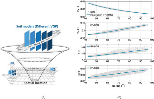
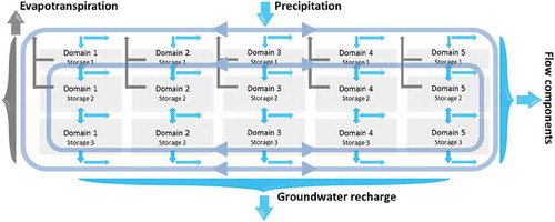
Figure 2. Schematic description of the soil model DYVESOM. Several sub-models with different van Genuchten (1980) parameters are structured in parallel with (water flux) connections to each other. This scheme was applied for every spatial location/hydrological response unit.

The model structure of DYVESOM provides the required interfaces for calibrations at soil moisture and groundwater level. This means that the upper 5 cm of the soil are evaluated individually in order to meet the penetration depth of C-band frequencies. To achieve this without numerical problems, sub time steps had to be developed. These evaluations were performed for all DYVESOM parameterizations (domains). To compare with satellite-based soil moisture measurements, one average value over all domains was applied. A second interface was developed to allow calibration with groundwater-level data. Since the deepest soil storages are beyond the root zone, the outflows of these storages are only controlled by the actual water contents θ3 in combination with a unit gradient boundary condition. The outflows are considered to represent groundwater recharge. To find correlations with groundwater-level measurements, two approaches were taken. First, the simulated time series of soil water content θ3 was used for the correlation analyses, and second, the time series of the simulated groundwater recharge was used for correlation analyses.

To improve the multi-objective calibration of such a highly complex system, a lexicographic optimization strategy was used (Gelleszun et al. 2015, 2017) (see Section 2.3).

2.3 Extended lexicographic calibration strategy

Optimization procedures require numerical expressions in order to determine the quality of the simulation objectively. Such an expression is called an objective function. Since the effects of complex hydrological processes can hardly be evaluated within one single-objective function, the assignment sequence “(A) calibration parameters → (B) hydrological processes → (C) objective function” is indefinite. This indefinite sequence is bypassed by the lexicographic calibration strategy. It immediately applies objective functions that are individually suited for the calibration parameters.

The fundamental idea of the lexicographic calibration strategy is to determine an order of preference of objective functions prior to the calibration. This order is dependent on the scientific context, the focus of the project and the available data. If the preferences are established, the calibration parameters are grouped and treated with individual objective functions. The grouping allows implementing multi-objective targets, which are handled sequentially. On the other hand, the search space of the calibration parameters is reduced with the effect of less calculation time compared to global optimization methods using all parameters at the same time. Various optimization algorithms can be utilized with the lexicographic calibration strategy. The downhill simplex method (Nelder and Mead 1965) was used in this study. This algorithm converges reliably, provided that the surface of the search space is continuous and has an explicit minimum. A simplex is a geometric construct that consists of a set of n + 1 points in an n-dimensional parameter space. The smaller the dimension of the parameter space, the more reliable is the convergence of the downhill simplex method.

The list in Table 1 shows the calibration parameters of PANTA RHEI that are used in this study.

Table 1. Description of the applied calibration parameters of the PANTA RHEI model.

Parameter	Description
Os	Offset of infiltration function. This parameter shifts the function of infiltration capacity and therefore influences the amount of water that infiltrates into the first soil storage. The higher the value, the higher is the infiltration rate. Os is a parameter within the soil model DYVESOM.
Dr	Draining rate of the canopy storage. The draining rate influences the interception loss and therefore the volume of runoff. The higher the value, the faster the canopy storage drains, leading to more runoff. Dr is a parameter within the calculation of the evapotranspiration.
Pf	Factor that influences preferential flow in the soil and therefore accounts for the allocation between fast and slow interflow. The higher the value, the more preferential flow occurs. Pf is a parameter within the soil model DYVESOM.
Fv	Factor that accounts for the influence of vegetation development on the soil. The higher the value, the more smoothed is the influence of vegetation (depending on the growing season index). Fv is a parameter within the soil model DYVESOM.
Fp	Factor that influences percolation. The higher the value, the more water percolates into deeper soil storages, leading to more baseflow and less interflow. Fp is a parameter within the soil model DYVESOM.
Ki	Linear storage constant of fast interflow. The higher the value, the steeper are the hydrographs of fast interflow. Ki is a parameter within the calculation of runoff formation.

We used different objective functions aimed at different hydrological variables (Q, GW and θ). The objective functions are associated with calibration parameters that have sensitive influence. The individual objective functions are applied in dependence on the calibration step. In the first calibration step, the main preference is given to the volume of simulated discharge and long-term groundwater values. Nevertheless, the soil surface as the upper physical boundary of the model controls all subsequent processes. Therefore, the quality of simulated soil water content is taken into account in the first calibration step too. The second step focuses on the simulated time series of groundwater level and still considers the total volume. In the last step, fine tuning on the discharge time series is selected as preference. Descriptions of the multi-objective functions for each step are given in Table 2.

Table 2. Order of preference for the multi-objective (discharge Q, groundwater level GW and soil water content θ) lexicographic calibration strategy with the corresponding calibration steps, associated parameters of PANTA RHEI and applied objective functions.

Step	Parameter	Objective function
1	Os, Dr	Absolute volume error of Q multiplied with correlation of time series of θ and relative error of long-term monthly values of GW
2	Pf, Fv	Absolute volume error of Q multiplied with coefficient of determination of time series of GW
3	Fp, Ki	Model efficiency Elog of the logarithmic time series of Q

The time period 2001–2011 was selected for model calibration and validation due to data availability of Q, GW and θ. Results from lexicographic multi-objective calibrations were compared with results obtained by lexicographic single-objective calibrations. Descriptions of the single-objective functions for each step are given in Table 3.

Table 3. Order of preference for the single-objective (Q) lexicographic calibration strategy with the corresponding calibration steps, associated parameters of PANTA RHEI and applied objective functions.

Step	Parameter	Objective function, description
1	Dr, Os	Absolute error of Q between observed and simulated peaks multiplied with RMSE between logarithmic observed and simulated time series
2	Fp, Fv	RMSE between low-flow values of the observed and simulated time series. The low-flow values are determined dependent on the 40% percentile of the (observed) duration curve of non-exceedence
3	Pf, Ki	Model efficiency Elog of the logarithmic time series of Q

The entire study period was separated into five sub-periods, each of 2-year length (see Table 4). Each 2-year period was calibrated individually. A cross-validation for every parameter set obtained for the 2-year periods was executed with each of the other (four) periods. The start times of the simulations were set 4 years prior to the evaluation periods to avoid the influence of initial conditions.

Table 4. Periods of simulation and calibration. The start of simulation was always 4 years before the calibration start time in order to avoid influence of initial model conditions.

	Period of calibration
Label	Start	End
P1	01.11.2001	31.10.2003
P2	01.11.2003	31.10.2005
P3	01.11.2005	31.10.2007
P4	01.11.2007	31.10.2009
P5	01.11.2009	31.10.2011
P6	01.11.2001	31.10.2011

Additional calibrations applied with the global optimization algorithm SCE-UA (Duan et al. 1992) were used as references. The SCE-UA is a renowned algorithm and often applied in hydrological calibration routines (Durner et al. 2007, Muttil and Jayawardena 2008, Zhang et al. 2009, Beskow et al. 2013, Guo et al. 2013). This algorithm is able to detect the global minimum within a multi-criteria optimization task (see e.g. Duan et al. 1994).

We developed one single- and one multi-objective function, which were used for the optimization with the global method SCE-UA. These functions include all criteria listed in Tables 2 and 3 with equal weights.

Several common quality criteria (see e.g. Hall 2001) were used to evaluate the calibration results. With respect to the discharge Q, the quality criteria E_rel, d and PBIAS were calculated in addition to E_log, which is the model efficiency (Nash and Sutcliffe 1970) based on logarithmic time series. These criteria were calculated for both model areas and all time periods. The criterion E_rel stands for model efficiency with relative errors and d is the index of agreement. These criteria are dimensionless and have their optimum at a value of 1.0. PBIAS (%) gives the percentage deviation in total volume. Since a hydrological model does not account for the simulation of groundwater level and groundwater flow, we applied straightforward transfer functions to generate a relative temporal course of groundwater level. Therefore, two different model results served as variables. The first is the simulated soil water content of the deepest soil storage (θ3), and the other is the simulated groundwater recharge (GWR). Both should be positively correlated to the groundwater level, if the hydrological model is plausible. To evaluate the model performance with respect to the groundwater level, the coefficient of determination R² was calculated in different ways: R²_θ3 compares the time series of simulated soil water content of the deepest soil storage with the time series of measured groundwater level, where both time series were standardized; R²_GWR uses both standardized time series of simulated groundwater recharge and the time series of measured groundwater level; and R²_GWRM is based on long-term mean monthly values of both standardized simulated groundwater recharge and measured groundwater level. With respect to the upper soil water content, θ, R² and E_rel were calculated based on the simulated and measured time series. Since the absolute values for the satellite-based measurements of θ are not reliable, a relative comparison (e.g. in the form of R² or E_rel) should be preferred (Mladenova et al. 2010, Liu et al. 2011). Sub-catchments with more than 20% forest area were not considered for the evaluation of θ, because the satellite sensors used operated in C-band frequencies.

2.4 Study areas

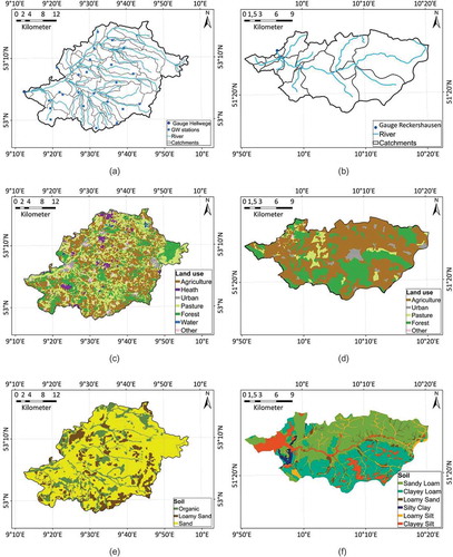
Two mesoscale catchments in northern Germany were selected as study areas. The catchments differ from each other in terms of their physiogeographical properties. The land use of the Hellwege catchment is mostly agricultural and based on a livestock economy. The Reckershausen catchment, in contrast, is dominated by arable land. The soil characteristics are also different: Hellwege has mostly sandy soils, which is typical for the landscape in the Lüneburger Heide,⁶ while the soils in Reckershausen are mostly fine grained. The spatial resolution of the soil map is 1:50 000. The spatial resolution of vegetation information (German ATKIS system) varies between 0.5 and 1 km² per polygon. In addition to soil and vegetation data, a 5 m × 5 m digital elevation model⁷ was used. Further, the authors are familiar with the behaviour of the hydrological systems of these two catchments (Hölscher et al. 2012, 2014, Wurpts 2014). Figure 3 presents maps of both catchments showing the spatial distribution of land use and soil properties, as well as the main rivers and locations of groundwater stations. The relevant regional properties are summarized in Table 5.

Figure 3. Spatial distribution of the main rivers and locations of (a, b) hydrometric and groundwater stations, (c, d) land use and (e, f) soil properties for (a, c, e) Hellwege and (b, d, f) Reckershausen.

2.5 Meteorological and remote sensing data

The meteorological input data (precipitation, average temperature, minimum and maximum temperature, relative humidity, global radiation and wind speed) were available at a daily time step.⁸ Data from 771 stations for precipitation and 123 stations for the other meteorological variables were used to generate 1 km × 1 km gridded data fields for Lower Saxony by means of geo-statistical analyses.⁸ Continuous discharge data⁸ for the two stations, Hellwege and Reckershausen, were available for the considered time periods (see Section 2.3) at a daily time step.

Satellite-based data were used for the comparison of simulated and observed soil water content. Processed satellite data originating from three different satellites were applied. The main properties of these products are summarized in Table 6. The ESCAT and ASCAT time series were spatially refined in dependence of the ASAR data (Kreye 2015). The strength of the ESCAT and ASCAT satellite data is the high temporal cover, while ASAR⁹ clearly has the better spatial resolution. The refinement was done in two steps. First, the times had to be identified where both satellite products have measurements within a ±6 h time frame. These matches were filtered again. Only matches with daily precipitation less than 1 mm were further considered. In a second step, regression analyses were conducted to detect a relationship between both satellite products. For these analyses, a genetic algorithm for the free adjustment of polynomial functions was applied. Finally, the ASCAT data were spatially downscaled in dependence of the ASAR data.

Table 5. Main physiogeographical properties of the two study areas, Hellwege and Reckershausen.

Property	Hellwege	Reckershausen
Area (km^2)	907	321
Main land use	37% arable land, 32% pasture, 21% forest, 10% other	61% arable land, 29% forest, 10% other
Soil properties	80% pure and loamy sand, 20% organic soil	55% clayey loam, 45% sandy loam
Elevation (m a.s.l.)	12–121	186–470
Mean discharge, 1970–2000 (m^3 s^−1)	9.13	2.59
Mean precipitation, 1970–2000 (mm)	837	785
Mean temperature, 1970–2000 (°C)	8.8	8.1
Number of HRUs	1778	294
Spatial resolution (km^2/HRU)	0.51	1.06

Table 6. Main properties of the applied satellite products of soil water content measurements. ERS-2: European Remote Sensing satellite 2; MetOP-A: Meteorological Operational Platform; Envisat: environmental satellite. ESCAT: advanced microwave instrument scatterometer; ASCAT: advanced scatterometer; ASAR: advanced synthetic aperture radar.

Satellite	Instrument	Run time	Spatial resolution	Temporal resolution
ERS-2	ESCAT	1996–2006	50 km × 50 km	~7 d/measurement
MetOP-A	ASCAT	2007–2020	25 km × 25 km	~1–2 d/measurement
Envisat	ASAR	2002–2012	1 km × 1 km (global mode)	~20 d/measurement

Sub-catchments with more than 20% forest cover were not considered, because the dense vegetation cover blocks C-band frequencies (see e.g. Wagner et al. 1999a, Mladenova et al. 2010). Measurement data at times with air temperature equal to and smaller than 0°C were not considered due to possible frozen soil. If the water in the upper centimetres of the soil is frozen, satellite-based measurements are not valid (Pathe et al. 2009, Mladenova et al. 2010).

Groundwater-level data were available for the Hellwege study area at 24 stations and an average temporal resolution of three weeks.⁸ These 24 time series were arithmetically merged to one time series being valid for the catchment since the sandy aquifer is highly permeable, hydraulically continuously connected and it is located near the (mostly flat) surface (Kreye 2015).

2.6 Latin hypercube sampling (LHS)

Uncertainty and sensitivity analyses are closely related and they overlap in many applications. While sensitivity analyses primarily quantify the influence of model parameters on model results, uncertainty analyses include other variables, such as the variation of input data (Loucks et al. 2005). An uncertainty analysis indirectly accounts for the sensitivity of the parameters. An essential goal of uncertainty analyses is the description of the bandwidth of possible model results by means of probability analysis (Loucks et al. 2005). In this study, the uncertainty analysis was limited to the variation of model parameter combinations and their effects on the model results and objective functions. The influence of the essential external variable (precipitation height) for the PANTA RHEI model system has already been described by Gelleszun et al. (2015).

To quantify the uncertainties of the model parameters and their influence on the model results, a large number of randomly generated model parameter combinations is needed. An established sampling method is the Monte Carlo method, while a more efficient method is the Latin hypercube sampling (LHS), first developed by McKay et al. (1979). According to Yu et al. (2001), LHS needs about 10% of the samples compared to the Monte Carlo method. Further information about LHS can be found in e.g. Loh (1996) or Xu et al. (2005). In this study, LHS was used to compare the results of the two optimization approaches (SCE-UA and lexicographic) with a random sample of parameter values from a multidimensional distribution. We evaluated how the calibrated parameter values differ from the values obtained by LHS. Second, the model performance based on the lexicographic and SCE-UA approaches can be benchmarked.

Latin hypercube sampling was performed for the Reckershausen model area, with 100 000 runs by varying all six model parameters. The time from 2003 to 2009 was selected as the simulation period, while only the last two years were used for analysis in order to minimize the influence of the initial conditions.

3 Results

3.1 Multi-objective calibration results

Calibration results are shown for the five different 2-year periods and for the entire period (2001–2011). Further, multi-criteria calibration (Q, GW and θ) was compared with single-criterion calibration (Q).

Table 7 shows the results for established quality criteria regarding the multi-criteria calibrations with the lexicographic strategy (see also Section 2.3). The calculations of these criteria are based on simulated and observed time series of Q, GW and θ. Regression functions based on these two indicators (θ3 and GWR) were fitted to the observed groundwater level. The quality of these regression functions was evaluated as R² of the time series “z” or as R² based on monthly mean values “m”. The individual calibration results mostly reached high scores. In Hellwege, the values of E_log, E_rel and d (with respect to Q) were slightly lower for the period 2009–2011 than for the other periods, but the volume (PBIAS) simulation was reasonable. A similar configuration was found for the period 2005–2007 in the study area of Reckershausen. High to moderate scores were realized for the comparison of measured and simulated groundwater levels, which are represented by the model output θ3. The R² and E_rel based on simulated and observed time series of θ achieved moderate scores in most cases. The winter months (December–February) were not considered when calculating the quality criteria of θ shown here. The reasons for this are given in Section 3.2.

Table 7. Quality criteria of the multi-objective calibration results obtained by the lexicographic calibration strategy for the whole period (2001–2011) and the five individual 2-year periods for the Hellwege and Reckershausen study areas. E_log: model efficiency based on logarithmic time series; E_rel: relative model efficiency; d: index of agreement; PBIAS: percentage volume error (%); and R²: coefficient of determination based on different time series.

	Q				GW			θ
	Elog	Erel	d	PBIAS	R^2θ3	R^2GWR	R^2GWRM	R^2	Erel
Hellwege
2001–2011	0.84	0.87	0.96	0.94	0.88	0.58	0.63	0.91	0.73
2001–2003	0.89	0.89	0.96	1.18	0.97	0.75	0.80	0.85	0.85
2003–2005	0.79	0.81	0.95	−0.59	0.51	0.31	0.42	0.54	0.39
2005–2007	0.81	0.81	0.96	−0.80	0.91	0.62	0.63	0.55	0.64
2007–2009	0.94	0.96	0.99	1.95	0.97	0.70	0.71	0.54	0.53
2009–2011	0.82	0.83	0.93	−0.18	0.89	0.49	0.50	0.44	0.64
Reckershausen
2001–2011	0.92	0.96	0.96	−1.55	-	-	-	0.86	0.85
2001–2003	0.94	0.96	0.97	1.56	-	-	-	0.84	0.94
2003–2005	0.94	0.95	0.97	−1.83	-	-	-	0.71	0.81
2005–2007	0.86	0.91	0.91	0.10	-	-	-	0.48	0.55
2007–2009	0.96	0.97	0.97	1.25	-	-	-	0.54	0.58
2009–2011	0.95	0.97	0.98	−3.56	-	-	-	0.54	0.72

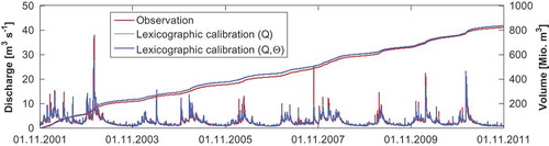
The observed and simulated discharge time series and cumulative time series for the Hellwege study area are shown in Figure 4. The simulations were based on the lexicographic calibration strategy with the single criterion (Q) and multi-criteria (Q, GW and θ). For both single- and multi-criteria calibrations, the simulated discharges are highly correlated with the observations. The a priori defined criteria of the preference order were fulfilled. As shown in Table 7, and Figures 4 and 5, high-flow and low-flow periods, as well as the seasonality, were simulated by the model with high accordance to the observed values. The multi-criteria calibration shows a slightly better fit regarding the volume, which also leads to an enhanced fit of the discharge peaks. Figure 5 shows the observed and simulated discharge time series and cumulative time series for the Reckershausen study area. Analogous to Hellwege, the simulated time series are very close to the observations. It is notable that there is no difference in the calibrated model result of the discharge time series between single-criterion fitting (Q) and multi-criteria fitting (Q, θ).

Figure 4. Hellwege: Discharge time series and cumulative time series of observations (red) and simulation based on lexicographic calibration for the period 2001–2011. The calibration (grey) is based on the single criterion Q and the calibration (blue) is based on the multi-criteria Q, GW and θ. For colour, see the online version.

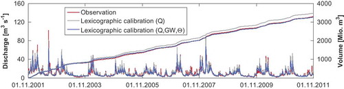
Figure 5. Reckershausen: Discharge time series and cumulative time series of observations (red) and simulation based on lexicographic calibration for the period 2001–2011. The calibration (grey) is based on the single criterion Q and the calibration (blue) is based on the multi-criteria Q and θ. For colour, see the online version.

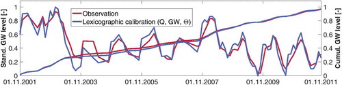
The simulation results of the Hellwege study area for standardized groundwater level are illustrated in Figure 6. The results shown in both Figures 4 and 6 are based on the final lexicographic calibration run. It is noteworthy that the large-scale hydrological model does not account for a calculation of groundwater flow as is done in specialized groundwater models. Nevertheless, the hydrological model performed very well in approximating the groundwater level. The seasonality and the cumulative time series of the simulation are highly correlated with the observations.

Figure 6. Hellwege: Standardized groundwater-level time series and cumulative time series of observations (red) and simulation based on lexicographic calibration (blue) for the period 2001–2011. For colour, see the online version.

Figure 7 shows the evaluation of the simulated soil water content θ for the upper 5 cm of soil storage based on the same calibration parameters as the results for Q and GW (Figs 4 and 6). The water content θ is defined as the effective saturation of the pore volume with a range between zero (dry) and one (saturated). The simulation is based on the multi-objective lexicographic calibration, while the observation is based on integrated satellite measurements of ESCAT/ASCAT/ASAR (Kreye 2015).

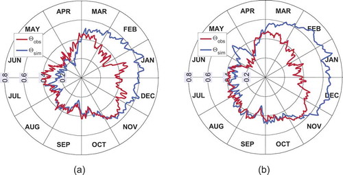
Figure 7 shows the long-term mean daily values of θ based on the period 2001–2011. Most of the year, the simulation and satellite-based observations in both study areas coincide very well. In winter, we generally observe a mismatch between simulated and measured soil water content. This seasonal effect is higher than expected, although we know that absolute values of satellite-based soil moisture measurements are often biased (Drusch et al. 2004, Pathe et al. 2009, Liu et al. 2011). Also, the (relative) dynamics of soil water content vary clearly in winter-time.

Figure 7. Simulated and observed soil water content (θ) as long-term mean daily values based on the period 2001–2011 for (a) Hellwege and (b) Reckershausen.

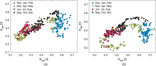
Scatter plots were created to further investigate this phenomenon and are shown in Figure 8. The simulated values are expressed as long-term mean daily values based on the period 2001–2011. The simulation is based on the multi-objective lexicographic calibration, while the observation is based on integrated satellite measurements of ESCAT/ASCAT/ASAR (Kreye 2015). The data points in the scatter plots are distinguished by means of the seasons. For both model areas, the highest agreement between simulation and observation can be seen in the autumn (September–November). During the winter months there is no correlation identifiable (blue dots in Fig. 8). It is assumed that this imbalance with respect to the seasons could be caused by frozen water in the upper soil layers, since satellite measurements are not valid if the soil water is frozen (see Albergel et al. 2009, Parajka et al. 2009, Pathe et al. 2009).

Figure 8. Scatter plot of simulated and observed soil water content (θ) as long-term mean daily values based on the period 2001–2011 for (a) Hellwege and (b) Reckershausen. The data points are coloured with respect to the season of the year. For colour, see the online version.

3.2 Representativity of the lexicographic calibration results and comparison with SCE-UA-based calibration results

3.2.1 Effects on the ranges of calibrated parameters

Ten different sets of model parameters were determined for both the lexicographic calibration strategy and for the SCE-UA, since every 2-year period was calibrated individually and both single- (Q) and multi-objective (Q, GW and θ) functions were used. Based on recent investigations, there was no change in the general hydrological response in the Hellwege and Reckershausen study areas within the period 2001–2011 (Hölscher et al. 2012, Hölscher et al. 2014, 2017, Wurpts 2014, Kreye et al. 2017). The values of the parameters originating from the calibrations of the 2-year periods are therefore anticipated to be similar. Figure 9 evaluates the ranges of the model parameters (see Tables 2 and 3) that were determined in the mentioned calibrations. The bandwidths of the parameters O_s, D_r, F_v and F_p are much smaller for the multi-objective calibration compared to the single-objective calibration for Hellwege, while the bandwidths of K_i and P_f are smaller for the single-objective calibration. This finding was expected since the first four parameters have more influence on the groundwater recharge than the latter two, and groundwater was considered within the multi-objective calibration. Different findings were obtained for Reckershausen. Here, the bandwidths of the parameters of single- and multi-objective calibrations are nearly identical. The multi-objective calibration was based on Q and θ. In conclusion, the consideration of θ did not influence the parameter bandwidths of the calibration.

In the Hellwege study area, the lexicographic calibration significantly reduced the bandwidths of O_s, D_r, F_p and K_i, in contrast to the SCE-UA calibration. The same effect may be observed for the Reckershausen study area, but for the parameters O_s, F_p and P_f. Hence, the lexicographic calibration strategy generally resulted in closer parameter bandwidths, although not all parameters showed closer bandwidths. Furthermore, the catchment has influence on the specific parameters that showed a reduced bandwidth. Obviously, the model parameters influence simulation results in different ways due to diverse physiographical structure and hydrological behaviour of the catchment. Close parameter bandwidths of the lexicographic calibration originate from a high influence of parameters on the results. These dominant parameters are indirectly identified by the lexicographic calibration expressed as close bandwidths and therefore high reliability.

3.2.2 Cross-validation

For the cross-validation, quality criteria were analysed for both study areas and calibration variants (lexicographic and SCE-UA). The criteria, which are shown in Table 7, are calculated for every 2-year period based on all final multi-objective calibration parameters. The scores of these quality criteria are visualized in Figure 10. Regarding Q, 90 quality criteria values for each model area are shown for five different calibration parameter sets (originating from the five 2-year periods) applied on six time periods (see Table 4) for three different quality criteria (E_log, E_rel and d). These criteria obtained slightly higher validation scores based on the lexicographic calibration strategy compared to SCE-UA. Regarding GW and θ, 90 and 60 criteria values are shown, respectively. The scores for GW are clearly higher for the lexicographic strategy. Regarding θ, there is hardly any difference between the scores of the lexicographic calibration strategy and SCE-UA.

In summary, both calibration methods (lexicographic and SCE-UA) gave high-quality criteria in validation. It can also be noted that the lexicographic calibration has higher scores in validation and closer parameter bandwidths in contrast to SCE-UA. These results show that the lexicographic calibration is capable of increasing the representativeness and reliability of the calibration parameters.

3.2.3 Effects on long-term monthly groundwater recharge

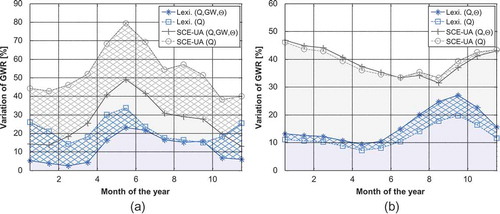
As shown in Figure 9, the calibration parameters vary in certain ranges, which also leads to different validation scores (Fig. 10). In order to investigate further the effects of the calibration parameters on model results, we analysed the seasonal variation of simulated groundwater recharge. Figure 11 shows these variations as long-term monthly mean values for the period 2001–2011. Groundwater recharge was simulated for this period several times based on the different calibration parameters originating from the five 2-year periods. This was done for the five lexicographic parameter sets based on single- (Q) and multi-objective (Q, GW, and θ) calibrations in each case. The same was elaborated based on the equivalent SCE-UA calibrations. The variations in long-term monthly groundwater recharge are expressed as absolute percentage deviations. Hence, a variation of e.g. 0% means that all simulations based on the different parameterizations yielded the same groundwater recharges. First, looking at the results for Reckershausen (Fig. 11(b)): distinctions can be observed between the lexicographic calibrations, with variations of 12% and 16% as yearly averages, for single- and multi-objective calibrations, respectively, and the SCE-UA calibrations, with variations of 39% as yearly averages for both calibrations. Hence, the lexicographic approach leads to a massive reduction of variations in simulations of groundwater recharge. However, there is no real difference regarding single- (Q) and multi-objective (Q, θ) calibrations in the Reckershausen study area. The consideration of θ did not enhance the calibration performance. Within the lexicographic calibration, it even increased the variation of groundwater recharge slightly (from 12% to 16%). The consideration of GW, in contrast, leads to a clear reduction of variation in the simulated groundwater recharge (cf. Hellwege, Fig. 11(a)). The variation is halved for the multi-objective calibrations in comparison to the single-objective calibrations. Further, the lexicographic calibration leads to approximately one-third of the variation when compared to SCE-UA. The average yearly variations based on the lexicographic calibrations were 22% (Q) and 11% (Q, GW and θ) and those based on SCE-UA were 54% (Q) and 27% (Q, GW and θ).

Figure 9. Box-and-whisker plots for parameter ranges based on the five different calibration periods for (a) Hellwege and (b) Reckershausen. A parameter range of 0% means that all five parameters have the same value. The lexicographic calibration results (blue) and those of calibration with SCE-UA (grey) are light for single-objective calibration (Q) and dark for multi-objective calibration (Q, GW, θ resp. Q, θ). For colour, see the online version.

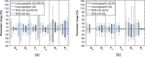
Figure 10. Box-and-whisker plots of various quality criteria (see Table 7) of (a, b) Q, (c) GW and (d, e) θ for (a, c, d) Hellwege and (b, e) Reckershausen. The simulation time series are based on the multi-objective lexicographic (blue) and SCE-UA (grey) calibration. The whiskers determine the maximum and minimum extent; the horizontal line represents the median; the outlined boxes are the 10% and 90% quantiles; and the filled boxes are the 25% and 75% quantiles. For colour, see the online version.

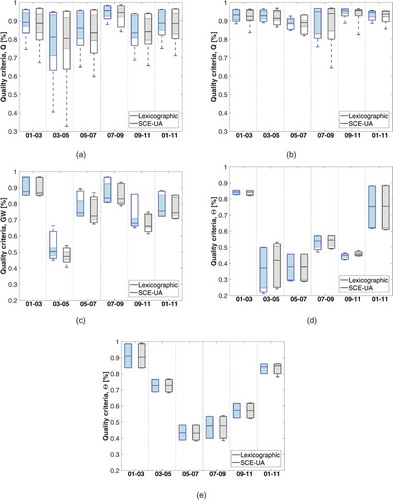
Figure 11. Seasonal variation of simulated groundwater recharge shown as long-term monthly mean values for the period 2001–2011 for (a) Hellwege and (b) Reckershausen. Results are based on the five 2-year lexicographic calibrations (blue) and the five 2-year SCE-UA calibrations (grey), with multi-objective results displayed as asterisks and crosses, respectively, and single-objective results as rectangles and circles, respectively. For colour, see the online version.

To summarize: (a) the lexicographic calibration delivers parameter sets that have similar effects on the hydrological system; (b) the consideration of groundwater level is a clear benefit; while (c) the consideration of satellite-based soil moisture seems to have no significant effect on the resulting parameters and model results.

3.3 Comparison with simulation runs based on LHS

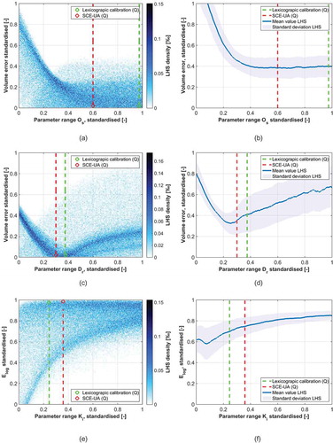
The LHS (see Section 2.6) was performed for the Reckershausen study area with 100 000 runs, varying all six model parameters. Figure 12 shows the relationship between various calibration parameters and objective functions based on the LHS runs. Figure 12(a) and (b) visualizes the connection between both standardized O_s and the absolute volume error. Figure 12(a), (c) and (e) displays the point density based on a scatter plot using the results of all 100 000 runs, while Figure 12(b), (d) and (f) shows the mean value and standard deviation of the volume error depending on O_s. All graphs include the parameter values of the single-objective lexicographic and SCE-UA calibrations. The single objective was selected due to the negligible influence of θ in the calibration. The relationship between parameter value and objective function is blurred due to the multiple variations of all calibration parameters in the LHS, but it can be seen that parameter values of O_s in the upper 50% of the parameter range yielded lower volume errors. The relationship between D_r and volume error is shown in Figure 12(c) and (d); it is stronger, with a quite clear minimum of the volume error. Both calibration variants are close to the parameter value of D_r for this minimum. The relationship between both standardized K_i and E_log is shown in Figure 12(e) and (f); it can be seen that the higher the parameter value, the better is the value of E_log. The two calibration variants yielded K_i values in the central part of the parameter range. Due to the influence of the other five parameters, different values of K_i can be used to achieve high values of E_log.

Figure 12. Relationships between standardized calibration parameters and objective functions based on 100 000 LHS runs. All graphs are based on the period 2007–2009 for the Reckershausen study area. (a, b) Relationships between the calibration parameter O_s and the absolute volume error. In (a, c, e), the point densities are calculated based on scatter plots. In (b, d), the average values and standard deviations of the volume error are shown in dependence on O_s and D_r. (e, f) the same analyses based on the calibration parameter K_i and the objective function E_log.

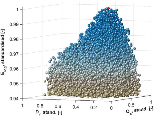
Figure 13 illustrates the relationship between standardized O_s, D_r and E_log based on the 100 000 LHS runs. Every sphere symbolizes one LHS run. In addition, the results of the single-objective lexicographic and SCE-UA calibrations are included. It can be seen that the SCE-UA calibration achieved the highest benchmark score in E_log, but the lexicographic calibration is very close to this score. It is worth noting that the conduction of the 100 000 LHS runs for the 6-year simulation in the Reckershausen study area took about 486 days on an i7 6 × 3.4 GHz processor. The SCE-UA algorithm needed on average 1300 iterations for one optimization task. This took about 6.3 days. The lexicographic calibration, in contrast, needed on average 80 iterations, which took only 0.4 days.

Figure 13. Relationship between standardized O_s and D_r calibration parameters and E_log objective function based on 100 000 LHS runs. Each sphere symbolizes one LHS run. In addition, the results of the single-objective lexicographic (green) and SCE-UA (red) calibrations are included. The graph is based on the period 2007–2009 for the Reckershausen study area. For colour, see the online version.

4 Summary

The main objective of this study was to identify representative parameter sets for two catchments, Reckershausen and Hellwege, in northern Germany by including groundwater-level measurements and satellite-based soil moisture in addition to flow data in an extended lexicographic calibration process. The integration of these additional data demanded a detailed soil water description within the hydrological model, with its corresponding parameters as appropriate interface to the optimization procedure. Therefore, we developed an innovative soil water model (DYVESOM), which was implemented in the hydrological modelling system PANTA RHEI. The DYVESOM model has the advantage of considering subgrid spatial variability of soil hydraulic parameters without the need of experimentally derived parameters (Kreye and Meon 2016), which therefore allows it to be applied on meso- or macroscale catchments. The upper 5 cm of the soil are evaluated individually in order to meet the penetration depth of C-band frequencies. Since the deepest soil storages are beyond the root zone, the outflows of these storages are controlled only by the actual water contents θ3 in combination with a unit gradient boundary condition. Therefore, the simulated time series of soil water content θ3 in the deepest soil storages was used to find correlations with groundwater-level measurements.

The two study catchments were calibrated by using a lexicographic calibration strategy. We integrated measurements of discharge, groundwater level and soil moisture in order to identify representative parameter sets for the catchments. For the calibration and subsequent validation, the observed time series were split into five sub-series, each of length 2 years. This procedure allowed a comparison to be made of the calibration methods and aimed for the obtained parameter sets to be representative of the catchments. The criteria for representativeness were goodness of fit for the validation periods, and the similarity of the resulting parameters and their effect on components of the water balance. Since we considered the same catchment but different time periods, we expected to identify similar parameters for the different periods.

Four variants of calibration procedure were distinguished: single- and multi-objective lexicographic calibration and single- and multi-objective calibration with SCE-UA. In general, both the lexicographic and SCE-UA calibrations provided high goodness-of-fit criteria for single- and multi-objective calibration. The results of the cross-validation and the identifiability of the parameter sets were more convincing for the lexicographic calibration strategy. Furthermore, the different lexicographic parameter sets resulted in similar effects on the hydrological system, which was indicated by comparing the monthly long-term groundwater recharge. These findings emphasize the high representativeness of the parameter sets for the hydrological model determined by the lexicographic calibration strategy.

5 Conclusions

5.1 Consideration of groundwater-level measurements in the calibration routine

The consideration of groundwater-level measurements within the calibration procedure turned out to be a clear benefit for the identifiability of the parameters. Regression analyses were conducted to find correlations between measured time series of groundwater level and simulated variables of the model. The strongest correlations were found by using the water content θ3 of the deepest soil storages. The groundwater level was calculated for θ3 based on a linear transfer function. Hence, the calibration process was improved by involving groundwater-level data due to fewer degrees of freedom of the calibration parameters. This is in accordance with other studies (e.g. Seibert 2000, Seibert and McDonnell 2002, Madsen and Khu 2006). Furthermore, the reliability of the simulated soil water budget could be increased. A very important point is that the calculation of groundwater recharge is much more plausible if measured groundwater levels are involved in the calibration.

It has to be acknowledged again that groundwater level was approximated with a hydrological model without the additional application of a groundwater model. In this context, the high agreement between approximated and measured groundwater levels is remarkable. Groundwater models require detailed data about the underground structure (geology) and have huge computation times. Hence, these models are limited to smaller areas. The possibility to apply a hydrological model for the approximation of groundwater level seems to be a promising alternative to complex model coupling (see e.g. Sutanudjaja et al. 2014, Maxwell et al. 2015). One constraint surely is that the groundwater has to be in hydraulic connection with the unsaturated zone and the geology must not be too complex.

5.2 Consideration of satellite-based soil moisture in the calibration routine

The consideration of satellite-based soil moisture did not influence the calibration results in a significant way for the two considered catchments. This was surprising and is in contrast to several other studies (e.g. Parajka et al. 2006, 2009, Sutanudjaja et al. 2014, Wanders et al. 2014, Laiolo et al. 2016, López López et al. 2016, Crow et al. 2017). Due to the specifications of the satellite measurements (C-band) used and the structure of our model, we conclude as follows.

• There is little margin in a physically-oriented model to provide a calibration parameter that modifies the relative soil water dynamics in the upper few centimetres significantly.

• The detected correlation between simulated and measured soil moisture is rather a correlation between spatially interpolated precipitation and measured satellite soil moisture.

Due to the low penetration depth of satellite-based soil moisture measurements, the comparison with simulated soil moisture was limited to the upper few centimetres of the soil. Even though the model provides possibilities to compare simulated to measured soil moisture values, it is of major importance that the model provides parameters that influence the objective within the calibration (reproduce the soil moisture in an adequate way). Rosnay et al. (2013) had similar findings, where model results are hardly affected when including the soil moisture in the calibration. If the aim is to obtain significant effects of calibration parameters on the relative soil water dynamics of the upper centimetres, there are two possibilities: either powerful parameters have to be imposed that dominate the whole physical background of the model, or the model structure itself has to be highly conceptual.

Precipitation directly influences the relative (and absolute) soil water dynamics in the upper few centimetres. Obviously, different soil hydraulic properties control the infiltration, but the signal of precipitation dominates in most cases. Draper et al. (2011) and Crow and Ryu (2009) concluded that satellite-based measurements of soil moisture could be used to improve the interpolation of precipitation. Crow et al. (2009) even presented a method to utilize satellite-based soil moisture retrievals to enhance satellite-based rainfall accumulation products.

In addition, our findings indicate that C-band satellite-based soil moisture measurements have to be considered with caution during winter months. Even after omitting the cold days (air temperature equal to or less than 0°C), the comparison between simulated and measured soil moisture showed no correlation in winter, in contrast to the high correlations with discharge and groundwater level. Apparently, this kind of filtering did not work properly for our catchments. The satellite-based measurements that remain after the application of the filter still seem to underestimate the soil moisture, which is analogous to the findings of Pellarin et al. (2006).

Considering the aforementioned aspects, we generally concluded that the use of C-band satellite-based soil moisture measurements for process-based hydrological model calibration gave no clear-cut benefit in the two considered catchments, Reckershausen and Hellwege. Some studies alternatively apply the soil water index SWI. But, due to the empirical calculation of the SWI by applying a simple low-pass filter, the valid localization (upper few centimetres) of the satellite measurement is blurred. We suggest using the SWI only for non-modelling applications to retrieve rough information about soil water on a supra-regional or global scale.

5.3 Performance of the multi-objective lexicographic calibration strategy

Reckershausen and Hellwege were categorized as mesoscale catchments. Generally, hydrological model applications on such large scales require enormous computing power (Zhang et al. 2009), which calls for time-efficient optimization methods. Besides the time efficiency, the advantage of the lexicographic calibration strategy is a consideration of expert knowledge prior to the simulation by determining a suitable order of preference. The objectivity was kept by applying automated optimization algorithms. The order of preference reasonably affects final outcome of the calibration, but in most cases this order is specified by the scientific context or engineering task. The results are repeatable, if the same order is applied. Generally, the individual definition of a suitable order can be compared to discover the most suitable parameter set in the context of a Pareto optimum by means of global multi-objective calibration.

The application of the extended hydrological model with the extended lexicographic calibration strategy on two catchments led to reliable and representative parameters, which was proved by analysing the impact of the parameters on model results via cross-validation and comparison to the well-established optimization algorithm SCE-UA (Duan et al. 1992). The cross-validation with different time periods also showed that the obtained parameter sets were very robust. This is important in hydrological modelling since we often deal with uncertain measurement data.

We showed that the SCE-UA optimization detects the “best” LHS sample regarding model performance. But it was also shown that the model performance based on the lexicographic approach is actually nearly identical to the best LHS sample. This is remarkable, because of the much shorter computation effort of the lexicographic approach compared to both SCE-UA and LHS. The lexicographic approach needs only 6% of the time of SCE-UA and 0.08% of the time of LHS.

One iteration run with the PANTA RHEI model on an average computer took 40 minutes. A global optimization run usually requires more than 1000 iterations, which adds up to more than 4 days of simulation time. For many practical applications in hydrology, large catchments with many hydrometric stations have to be addressed. The catchment of the River Aller in Lower Saxony (Germany), for instance, is the key study area in various projects funded by the state of Lower Saxony, Ministry of Environment, Energy and Climate Protection (Hölscher et al. 2012, 2014, 2017).¹⁰ This catchment has more than 150 hydrometric stations. It is obvious that calibration with the help of global optimization algorithms is not feasible because of the huge run time (4 days × 150 stations = 600 days). But with the help of a lexicographic calibration strategy, this task can be solved.

The similarity of the parameters and the cross-validation scores shown here, as well as the integration of groundwater-level data within the calibration process, indicate the good representativeness of the hydrological model and, furthermore, emphasize the application of multi-objective lexicographic calibration approaches.

Acknowledgments

We thank the Niedersächsischen Landesbetrieb für Wasserwirtschaft, Küsten- und Naturschutz (NLWKN), the Harzwasserwerke and the Leibniz University of Hannover for provision of the necessary data.

Disclosure statement

No potential conflict of interest was reported by the authors.

Additional information

Funding

The study was connected to the projects “Water management impact assessment of global climate change” (KLIBIW) phases 3 and 4, which were funded by the state of Lower Saxony, Ministry of Environment, Energy and Climate Protection.

Notes

¹ Advanced Microwave Scanning Radiometer for the Earth Observing System.

² Advanced scatterometer.

³ Soil Moisture and Ocean Salinity.

⁴ Shuffled Complex Evolution – University of Arizona.

⁵ API – application programming interface.

⁶ Lüneburger Heath.

⁷ Provided by the Lower Saxony Water Management, Coastal Defence and Nature Conservation Agency (NLWKN).

⁸ Executed by the Institute of Water Resources Management, Hydrology and Agriculture (WAWI) of the Leibniz University of Hannover.

⁹ Provided by the Department of Geodesy and Geoinformation of the TU Wien.

¹⁰ https://www.nlwkn.niedersachsen.de/startseite/wasserwirtschaft/sonderthemen_projekte/klimawandel/projekt_klibiw/das-projekt-klibiw-104191.html.

References

- Albergel, C., et al., 2009. An evaluation of ASCAT surface soil moisture products with in-situ observations in Southwestern France. Hydrology and Earth System Sciences, 13 (2), 115–124. doi:10.5194/hess-13-115-2009
- Albergel, C., et al., 2010. Cross-evaluation of modelled and remotely sensed surface soil moisture with in situ data in southwestern France. Hydrology and Earth System Sciences, 14 (11), 2177–2191. doi:10.5194/hess-14-2177-2010
- Al-Safi, H.I.J. and Sarukkalige, P.R., 2017. Assessment of future climate change impacts on hydrological behavior of Richmond River Catchment. Water Science and Engineering, 10 (3), 197–208. doi:10.1016/j.wse.2017.05.004
- Bárdossy, A. and Singh, S.K., 2008. Robust estimation of hydrological model parameters. Hydrology and Earth System Sciences, 12 (6), 1273–1283. doi:10.5194/hess-12-1273-2008
- Beskow, S., Norton, L.D., and Mello, C.R., 2013. Hydrological prediction in a tropical watershed dominated by oxisols using a distributed hydrological model. Water Resources Management, 27 (2), 341–363. doi:10.1007/s11269-012-0189-8
- Beven, K., 1995. Linking parameters across scales: subgrid parameterizations and scale dependent hydrological models. Hydrological Processes, 9 (5–6), 507–525. doi:10.1002/(ISSN)1099-1085
- Binley, A., Beven, K., and Elgy, J., 1989a. A physically based model of heterogeneous hillslopes: 2. Effective hydraulic conductivities. Water Resources Research, 25 (6), 1227–1233. doi:10.1029/WR025i006p01227
- Binley, A., Elgy, J., and Beven, K., 1989b. A physically based model of heterogeneous hillslopes: 1. Runoff production. Water Resources Research, 25 (6), 1219–1226. doi:10.1029/WR025i006p01219
- Boess, J., et al., eds., 2004. Erläuterungsheft zur digitalen nutzungsdifferenzierten Bodenkundlichen Übersichtskarte 1:50.000 (BÜK50n) von Niedersachsen. Stuttgart: Schweizerbart’sche Verlagsbuchhandlung.
- Bronstert, A. and Bárdossy, A., 1999. The role of spatial variability of soil moisture for modelling surface runoff generation at the small catchment scale. Hydrology and Earth System Sciences, 3 (4), 505–516. doi:10.5194/hess-3-505-1999
- Chen, D., et al., 2005. Comparison of the Thornthwaite method and pan data with the standard Penman-Monteith estimates of reference evapotranspiration in China. Climate Research, 28, 123–132. doi:10.3354/cr028123
- Christiaens, K. and Feyen, J., 2002. Constraining soil hydraulic parameter and output uncertainty of the distributed hydrological MIKE SHE model using the GLUE framework. Hydrological Processes, 16 (2), 373–391. doi:10.1002/(ISSN)1099-1085
- Coles, N.A., et al., 1997. Modelling runoff generation on small agricultural catchments: can real world runoff responses be captured? Hydrological Processes, 11 (2), 111–136. doi:10.1002/(SICI)1099-1085(199702)11:2<111::AID-HYP434>3.0.CO;2-M
- Crow, W.T., et al., 2009. Improving satellite-based rainfall accumulation estimates using spaceborne surface soil moisture retrievals. Journal of Hydrometeorology, 10 (1), 199–212. doi:10.1175/2008JHM986.1
- Crow, W.T., et al., 2017. L band microwave remote sensing and land data assimilation improve the representation of prestorm soil moisture conditions for hydrologic forecasting. Geophysical Research Letters, 44 (11), 5495–5503. doi:10.1002/2017GL073642
- Crow, W.T. and Ryu, D., 2009. A new data assimilation approach for improving runoff prediction using remotely-sensed soil moisture retrievals. Hydrology and Earth System Sciences, 13 (1), 1–16. doi:10.5194/hess-13-1-2009
- de Roo, A.P.J., Wesseling, C.G., and Ritsema, C.J., 1996. Lisem: a single-event physically based hydrological and soil erosion model for drainage basins. I: theory, input and output. Hydrological Processes, 10 (8), 1107–1117. doi:10.1002/(ISSN)1099-1085
- Draper, C., et al., 2011. Assimilation of ASCAT near-surface soil moisture into the SIM hydrological model over France. Hydrology and Earth System Sciences, 15 (12), 3829–3841. doi:10.5194/hess-15-3829-2011
- Drusch, M., et al., 2004. Soil moisture retrieval during the Southern Great Plains Hydrology Experiment 1999. A comparison between experimental remote sensing data and operational products. Water Resources Research, 40 (2), 687. doi:10.1029/2003WR002441
- Duan, Q., Sorooshian, S., and Gupta, V., 1992. Effective and efficient global optimization for conceptual rainfall-runoff models. Water Resources Research, 28 (4), 1015–1031. doi:10.1029/91WR02985
- Duan, Q., Sorooshian, S., and Gupta, V.K., 1994. Optimal use of the SCE-UA global optimization method for calibrating watershed models. Journal of Hydrology, 158 (3–4), 265–284. doi:10.1016/0022-1694(94)90057-4
- Duan, Q.Y., Gupta, V.K., and Sorooshian, S., 1993. Shuffled complex evolution approach for effective and efficient global minimization. Journal of Optimization Theory and Applications, 76 (3), 501–521. doi:10.1007/BF00939380
- Durner, W., Jansen, U., and Iden, S.C., 2007. Effective hydraulic properties of layered soils at the lysimeter scale determined by inverse modelling. European Journal of Soil Science, 071026202618002-???. doi:10.1111/ejs.ahead-of-print
- Efstratiadis, A. and Koutsoyiannis, D., 2010. One decade of multi-objective calibration approaches in hydrological modelling: a review. Hydrological Sciences Journal, 55 (1), 58–78. doi:10.1080/02626660903526292
- Entin, J.K., et al., 2000. Temporal and spatial scales of observed soil moisture variations in the extratropics. Journal of Geophysical Research, 105 (D9), 11865–11877. doi:10.1029/2000JD900051
- Förster, K., 2013. Detaillierte Nachbildung von Schneeprozessen in der hydrologischen Modellierung. Dissertation. Technische Universität Braunschweig, Leichtweiß-Institut für Wasserbau.
- Förster, K., et al., 2014. Effect of meteorological forcing and snow model complexity on hydrological simulations in the Sieber catchment (Harz Mountains, Germany). Hydrology and Earth System Sciences, 18 (11), 4703–4720. doi:10.5194/hess-18-4703-2014
- Förster, K., Gelleszun, M., and Meon, G., 2012. A weather dependent approach to estimate the annual course of vegetation parameters for water balance simulations on the meso- and macroscale. Advances in Geosciences, 32, 15–21. doi:10.5194/adgeo-32-15-2012
- Gelleszun, M., Kreye, P., and Meon, G., 2015. Lexikografische Kalibrierungsstrategie für eine effiziente Parameterschätzung in hochaufgelösten Niederschlag-Abfluss-Modellen. Hydrologie und Wasserbewirtschaftung, 59 (3), 84–95.
- Gelleszun, M., Kreye, P., and Meon, G., 2017. Representative parameter estimation for hydrological models using a lexicographic calibration strategy. Journal of Hydrology, 553, 722–734. doi:10.1016/j.jhydrol.2017.08.015
- Gocht, M., 2013. Optimierter Betrieb eines Talsperrenverbundsystems mit Anpassung an den Klimawandel. Braunschweig: Univ.-Bibl.
- Gocht, M. and Meon, G., 2016. Modelling and assessment of the combined impacts of climatic and demographic change on a multipurpose reservoir system in the Harz mountains. Environmental Earth Sciences, 75 (21), 3589. doi:10.1007/s12665-016-6099-y
- Guo, J., et al., 2013. A novel multi-objective shuffled complex differential evolution algorithm with application to hydrological model parameter optimization. Water Resources Management, 27 (8), 2923–2946. doi:10.1007/s11269-013-0324-1
- Hall, M.J., 2001. How well does your model fit the data? Journal of Hydroinformatics, 3 (1), 49–55. doi:10.2166/hydro.2001.0006
- Hasenauer, S., et al., 2009. Bodenfeuchtedaten aus Fernerkundung für hydrologische Anwendungen. Österreichische Wasser- und Abfallwirtschaft, 61 (7–8), 117–123. doi:10.1007/s00506-009-0097-1
- Hattermann, F.F., et al., 2017. Cross‐scale intercomparison of climate change impacts simulated by regional and global hydrological models in eleven large river basins. Climatic Change, 141 (3), 561–576. doi:10.1007/s10584-016-1829-4
- Holland, J.H., 1975. Adaptation in natural and artificial systems. An introductory analysis with applications to biology, control and artificial intelligence. Ann Arbor: University of Michigan Press.
- Hölscher, J., et al., 2012. Globaler Klimawandel. Wasserwirtschaftliche Folgenabschätzung für das Binnenland. 1st ed. Norden: NLWKN.
- Hölscher, J., et al., 2014. Globaler Klimawandel. Wasserwirtschaftliche Folgenabschätzung für das Binnenland. 1st ed. Norden: NLWKN.
- Hölscher, J., et al., 2017. Globaler Klimawandel. Wasserwirtschaftliche Folgenabschätzung für das Binnenland : gesamtbericht des Projektes KliBiW Themenbereich Hochwasser. 1st ed. Hannover: Niedersächsischer Landesbetrieb für Wasserwirtschaft Küsten- und Naturschutz (NLWKN).
- Jolly, W.M., Nemani, R., and Running, S.W., 2005. A generalized, bioclimatic index to predict foliar phenology in response to climate. Global Change Biology, 11 (4), 619–632. doi:10.1111/gcb.2005.11.issue-4
- Kirchner, J.W., 2006. Getting the right answers for the right reasons: linking measurements, analyses, and models to advance the science of hydrology. Water Resources Research, 42 (W03S04), 1–5. doi:10.1029/2005WR004362
- Koch, J., et al., 2016. Inter-comparison of three distributed hydrological models with respect to seasonal variability of soil moisture patterns at a small forested catchment. Journal of Hydrology, 533, 234–249. doi:10.1016/j.jhydrol.2015.12.002
- Kreye, P., 2015. Mesoskalige Bodenwasserhaushaltsmodellierung mit Nutzung von Grundwassermessungen und satellitenbasierten Bodenfeuchtedaten. Dissertation. Technische Universität Braunschweig.
- Kreye, P., et al., 2017. Detaillierte Nachbildung der Niedrigwasserverhältnisse in der hydrologischen Modellierung für die Ermittlung von Klimafolgen im Aller-Leine-Oker-Einzugsgebiet, Niedersachsen. Koblenz: Bundesanstalt für Gewässerkunde (BfG).
- Kreye, P., Gelleszun, M., and Meon, G., 2012. Ein landnutzungssensitives Bodenmodell für die meso- und makroskalige Wasserhaushaltsmodellierung. In: M. Weiler, ed.. Wasser ohne Grenzen. Freiburg/Breisgau: Rombach Druck- und Verlagshaus GmbH & Co. KG, 25–30
- Kreye, P., Gocht, M., and Förster, K., 2010. Entwicklung von Prozessgleichungen der Infiltration und des oberflächennahen Abflusses für die Wasserhaushaltsmodellierung. Hydrologie und Wasserbewirtschaftung, 54 (5), 268–278.
- Kreye, P. and Meon, G., 2016. Subgrid spatial variability of soil hydraulic functions for hydrological modelling. Hydrology and Earth System Sciences, 20 (6), 2557–2571. doi:10.5194/hess-20-2557-2016
- Laiolo, P., et al., 2016. Impact of different satellite soil moisture products on the predictions of a continuous distributed hydrological model. International Journal of Applied Earth Observation and Geoinformation, 48, 131–145. doi:10.1016/j.jag.2015.06.002
- Law, J., 1944. A statistical approach to the interstitial heterogeneity of sand reservoirs. Transactions of the AIME, 155 (1), 202–222. doi:10.2118/944202-G
- Le, T.T.H., et al., 2017. Räumliche und zeitliche Variabilität der Wassermenge und Wasserqualität des Thi-Vai-Einzugsgebietes in Südvietnam – datenanalyse eines Monitoringprogramms. Hydrologie & Wasserbewirtschaftung, 61 (6), 370–382.
- Leij, F., et al., 1996. The UNSODA unsaturated soil hydraulic database: user’s manual. Cincinnati, OH: National Risk Management Research Laboratory, Office of Research and Development, U.S. Environmental Protection Agency.
- Liu, Y.Y., et al., 2011. Developing an improved soil moisture dataset by blending passive and active microwave satellite-based retrievals. Hydrology and Earth System Sciences, 15 (2), 425–436. doi:10.5194/hess-15-425-2011
- Loh, W.-L., 1996. On Latin hypercube sampling. The Annals of Statistics, Singapore, 24 (5), 2058–2080. doi:10.1214/aos/1069362310
- López López, P., et al., 2016. Improved large-scale hydrological modelling through the assimilation of streamflow and downscaled satellite soil moisture observations. Hydrology and Earth System Sciences, 20 (7), 3059–3076. doi:10.5194/hess-20-3059-2016
- Lorenz, M., et al., 2014. Ecohydrological modeling of the Thi Vai Catchment in South Vietnam. In: G. Meon, et al., ed., EWATEC-COAST: technologies for environmental and water protection of coastal zones in vietnam. contributions to 4th international conference for environment and natural resources, ICENR 2014. Göttingen, Niedersachs: Cuvillier, E, 1–9
- Lorenz, M., 2015. Entwicklung eines ökohydrologischen Modellsystems auf der Einzugsgebietsskala und Anwendung in den sommerfeuchten Tropen. Braunschweig: Technische Universität Braunschweig.
- Loucks, D.P., et al., 2005. Water resources systems planning and management. An introduction to methods, models and applications. Paris: UNESCO.
- Löw, A., Bach, H., and Mauser, W., 2007. 5 years of ENVISAT ASAR soil moisture observations in southern germany. In: Proc. ENVISAT Symposium 23–27.04.2007, Montreux, Switzerland. ESA-SP636.
- LWI-HYWAG und IfW, 2012. Panta Rhei Benutzerhandbuch - Programmdokumentation zur hydrologischen Modellsoftware (unveröffentlicht).
- Madsen, H. and Khu, S., 2006. On the use of Pareto optimization for multi-criteria calibration of hydrological models. IAHS Publication, 304, 93.
- Maxwell, R.M., Condon, L.E., and Kollet, S.J., 2015. A high-resolution simulation of groundwater and surface water over most of the continental US with the integrated hydrologic model ParFlow v3. Geoscientific Model Development, 8 (3), 923–937. doi:10.5194/gmd-8-923-2015
- McKay, M.D., Beckman, R.J., and Conover, W.J., 1979. A comparison of three methods for selecting values of input variables in the analysis of output from a computer code. Technometrics, 21 (2), 239.
- Meon, G., et al., 2015. Innovative Hochwasservorhersage für kleine und mittlere Einzugsgebiete. In: M. Evers and B. Diekkrüger, eds..Forum für Hydrologie und Wasserbewirtschaftung. Aktuelle Herausforderungen im Flussgebiets- und Hochwassermanagement, Beiträge zum Tag der Hydrologie am 19./20. März 2015 an der Universität Bonn. Hennef, 287–296
- Meon, G., et al., 2017. Entwicklung einer Basisversion eines Managementsystems für die regionale Wasserwirtschaft einer Küstenzone in Vietnam. Hydrologie & Wasserbewirtschaftung, 61 (6), 437–449.
- Meon, G., Pätsch, M., and van Phuoc, N., 2014. EWATEC-COAST: technologies for environmental and water protection of coastal regions in vietnam. Contributions to 4th international conference for environment and natural resources—ICENR 2014. 1st ed. Göttingen, Niedersachs: Cuvillier, E.
- Merz, R., Parajka, J., and Blöschl, G., 2011. Time stability of catchment model parameters. Implications for climate impact analyses. Water Resources Research, 47 (2), 17. doi:10.1029/2010WR009505
- Meyer, S., 2013. Operationelle Hochwasservorhersage in Niedersachsen mit dem Wasserhaushaltsmodell PANTA RHEI. In: M. Casper, et al., eds.. Simulation hydrologischer Systeme - wie nah kommen wir der Realität? Beiträge zum 3. Trierer Workshop zur Niederschlag-Abfluss-Modellierung am 17. und 18. September 2012 in Trier. Hennef: Dt. Vereinigung für Wasserwirtschaft, Abwasser und Abfall, 287–296
- Mladenova, I., et al., 2010. Validation of the ASAR global monitoring mode soil moisture product using the NAFE’05 data set. IEEE Transactions on Geoscience and Remote Sensing, 48 (6), 2498–2508. doi:10.1109/TGRS.2010.2040746
- Monteith, J.L., 1965. Evaporation and environment. In: G.E. Fogg, ed. The state and movement of water in living organisms. Cambridge: Cambridge University Press, 205–234.
- Muttil, N. and Jayawardena, A.W., 2008. Shuffled Complex Evolution model calibrating algorithm: enhancing its robustness and efficiency. Hydrological Processes, 22 (23), 4628–4638. doi:10.1002/hyp.v22:23
- Nash, J.E. and Sutcliffe, J.V., 1970. River flow forecasting through conceptual models. Part I: a discussion of principles. Elsevier.
- Nelder, J.A. and Mead, R., 1965. A simplex method for function minimization. The Computer Journal, 7 (4), 308–313. doi:10.1093/comjnl/7.4.308
- Nemes, A., et al., 2001. Description of the unsaturated soil hydraulic database UNSODA version 2.0. Journal of Hydrology, 251 (3–4), 151–162. doi:10.1016/S0022-1694(01)00465-6
- Parajka, J., et al., 2006. Assimilating scatterometer soil moisture data into conceptual hydrologic models at the regional scale. Hydrology and Earth System Sciences, 10 (3), 353–368. doi:10.5194/hess-10-353-2006
- Parajka, J., et al., 2009. Matching ERS scatterometer based soil moisture patterns with simulations of a conceptual dual layer hydrologic model over Austria. Hydrology and Earth System Sciences, 13 (2), 259–271. doi:10.5194/hess-13-259-2009
- Pathe, C., et al., 2009. Using ENVISAT ASAR global mode data for surface soil moisture retrieval over Oklahoma, USA. IEEE Transactions on Geoscience and Remote Sensing, 47 (2), 468–480. doi:10.1109/TGRS.2008.2004711
- Pellarin, T., Calvet, J.-C., and Wagner, W., 2006. Evaluation of ERS scatterometer soil moisture products over a half-degree region in southwestern France. Geophysical Research Letters, 33, 17. doi:10.1029/2006GL027231
- Penman, H.L., 1948. Natural evaporation from open water, bare soil and grass. Proceedings of the Royal Society A: Mathematical, Physical and Engineering Sciences, 193 (1032), 120–145.
- Price, W.L., 1987. Global optimization algorithms for a CAD workstation. Journal of Optimization Theory and Applications, 55 (1), 133–146. doi:10.1007/BF00939049
- Qu, W., 2014. Characterization of soil water content variability at the catchment scale using sensor network and stochastic modelling. Dissertation. Forschungszentrum Jülich.
- Qu, W., et al., 2015. Predicting subgrid variability of soil water content from basic soil information. Geophysical Research Letters, 42 (3), 789–796. doi:10.1002/2014GL062496
- Riedel, G., et al., 2017. Erfahrung mit Radarprodukten bei der operationellen Hochwasservorhersage in Niedersachsen. KW - Korrespondenz Wasserwirtschaft, 10 (11), 664–671.
- Rosnay, P.D., et al., 2013. A simplified Extended Kalman Filter for the global operational soil moisture analysis at ECMWF. Quarterly Journal of the Royal Meteorological Society, 139 (674), 1199–1213. doi:10.1002/qj.2023
- Schaap, M.G., van Leij, J.F., and van Genuchten, M.T., 2001. ROSETTA: a computer program for estimating soil hydraulic parameters with hierarchical pedotransfer functions. Journal of Hydrology, 251 (3–4), 163–176. doi:10.1016/S0022-1694(01)00466-8
- Schewe, J., et al., 2014. Multimodel assessment of water scarcity under climate change. Proceedings of the National Academy of Sciences of the United States of America, 111 (9), 3245–3250. doi:10.1073/pnas.1222460110
- Seibert, J., 2000. Multi-criteria calibration of a conceptual runoff model using a genetic algorithm. Hydrology and Earth System Sciences, 4 (2), 215–224. doi:10.5194/hess-4-215-2000
- Seibert, J. and McDonnell, J.J., 2002. On the dialog between experimentalist and modeler in catchment hydrology: use of soft data for multicriteria model calibration. Water Resources Research, 38 (11). 23-1-23-14. doi:10.1029/2001WR000978
- Sentelhas, P.C., Gillespie, T.J., and Santos, E.A., 2010. Evaluation of FAO Penman–monteith and alternative methods for estimating reference evapotranspiration with missing data in Southern Ontario, Canada. Agricultural Water Management, 97 (5), 635–644. doi:10.1016/j.agwat.2009.12.001
- Skamarock, W.C., et al., 2008. A description of the advanced research WRF version 3, 27, 3–27. NCAR. doi:10.5065/D68S4MVH
- Sponagel, H., 2005. Bodenkundliche Kartieranleitung. Mit 103 Tabellen. 5th ed. Stuttgart: Schweizerbart.
- Sutanudjaja, E.H., et al., 2014. Calibrating a large-extent high-resolution coupled groundwater-land surface model using soil moisture and discharge data. Water Resources Research, 50 (1), 687–705. doi:10.1002/2013WR013807
- Sutanudjaja, E.H., et al., 2018. PCR-GLOBWB 2. A 5 arcmin global hydrological and water resources model. Geoscientific Model Development, 11 (6), 2429–2453. doi:10.5194/gmd-11-2429-2018
- Van Beek, L.P. and Bierkens, M.F., 2008. The global hydrological model PCR-GLOBWB: conceptualization, parameterization and verification. Utrecht: Utrecht University.
- van der Knijff, J.M., Younis, J., and Roo, A.P.J.D., 2010. LISFLOOD. A GIS‐based distributed model for river basin scale water balance and flood simulation. International Journal of Geographical Information Science, 24 (2), 189–212. doi:10.1080/13658810802549154
- van Genuchten, M.T., 1980. A closed-form equation for predicting the hydraulic conductivity of unsaturated soils. Soil Science Society of America Journal, 44 (5), 892–898. doi:10.2136/sssaj1980.03615995004400050002x
- Viera, S.R., et al., 2011. Characterizing the spatial variability of soil hydraulic properties of a poorly drained soil. World Applied Sciences Journal, 12 (6), 732–741.
- Wagner, W., et al., 1999a. A study of vegetation cover effects on ERS scatterometer data. IEEE Transactions on Geoscience and Remote Sensing, 37 (2), 938–948. doi:10.1109/36.752212
- Wagner, W., Lemoine, G., and Rott, H., 1999b. A method for estimating soil moisture from ERS scatterometer and soil data. Remote Sensing of Environment, 70 (2), 191–207. doi:10.1016/S0034-4257(99)00036-X
- Wanders, N., et al., 2014. The benefits of using remotely sensed soil moisture in parameter identification of large-scale hydrological models. Water Resources Research, 50 (8), 6874–6891. doi:10.1002/2013WR014639
- Wurpts, A., 2014. Forschungsthema 7: küste und Küstenschutz – A-Küst. In: F. Beese, et al., eds.. Abschlussbericht des Forschungsverbundes KLIFF – august 2014. Göttingen: Niedersächsisches Ministerium für Wissenschaft und Kultur, 84–103
- Xu, C., et al., 2005. Latin hypercube sampling and geostatistical modeling of spatial uncertainty in a spatially explicit forest landscape model simulation. Ecological Modelling, 185 (2–4), 255–269. doi:10.1016/j.ecolmodel.2004.12.009
- Yu, P.-S., Yang, T.-C., and Chen, S.-J., 2001. Comparison of uncertainty analysis methods for a distributed rainfall–runoff model. Journal of Hydrology, 244 (1–2), 43–59. doi:10.1016/S0022-1694(01)00328-6
- Zeunert, S., et al., 2017. Modellgestützte Untersuchungen der Auswirkungen des Klimawandels und fortschreitender anthropogener Entwicklungen auf die Wasserqualität des tropischen Thi-Vai-Ästuars. Hydrologie & Wasserbewirtschaftung, 61 (6), 424–436.
- Zhang, X., et al., 2009. Evaluation of global optimization algorithms for parameter calibration of a computationally intensive hydrologic model. Hydrological Processes, 23 (3), 430–441. doi:10.1002/hyp.7152
- Zhu, J. and Mohanty, B.P., 2002. Spatial averaging of van Genuchten hydraulic parameters for steady-state flow in heterogeneous soils: a numerical study. Vadose Zone Journal, 1 (2), 261–272. doi:10.2136/vzj2002.2610
- Zhu, J., Young, M.H., and van Genuchten, M.T., 2007. Upscaling schemes and relationships for the Gardner and van Genuchten hydraulic functions for heterogeneous soils. Vadose Zone Journal, 6 (1), 186. doi:10.2136/vzj2006.0041