Polynomial chaos expansion and response surface method for nonlinear modelling of reference evapotranspiration

ABSTRACT

The feasibility of polynomial chaos expansion (PCE) and response surface method (RSM) models is investigated for modelling reference evapotranspiration (ET₀). The modelling results of the proposed models are validated against the M5 model tree and multi-layer perceptron neural network (MLPNN) methods. Two meteorological stations, Isparta and Antalya, in the Mediterranean region of Turkey, are inspected. Various input combinations of daily air temperature, solar radiation, wind speed and relative humidity are constructed as input attributes for the ET₀. Generally, the modelling accuracy is increased by increasing the number of inputs. Including wind speed in the model inputs considerably increases their accuracy in modelling ET₀. Mean absolute error (MAE), root mean square error (RMSE), agreement index (d) and Nash-Sutcliffe efficiency (NSE) are used as comparison criteria. The PCE is the most accurate model in estimating daily ET₀, giving the lowest MAE (0.036 and 0.037 mm) and RMSE (0.047 and 0.050 mm) and the highest d (0.9998 and 0.9999) and NSE (0.9992 and 0.9996) with the four-input PCE models for Isparta and Antalya, respectively.

KEYWORDS:

• reference evapotranspiration
• polynomial chaos expansion
• MLPNN
• M5 model tree
• response surface method

Editor R. Woods Associate editor F.-J. Chang

1 Introduction

Evapotranspiration (ET) is an important part of the hydrological budget, which is associated with the energy and mass exchange between the water–soil system and the environment. A precise determination of the amount of water consumed by ET is a basic factor in increasing crop yield. Moreover, the estimation of ET has a decisive role in designing and determining the capacity of irrigation and drainage networks. In other words, ET is a necessary parameter for computing soil water balance and suitable irrigation scheduling, frequency of irrigation and even choosing a proper irrigation system. Considering the direct linkage between the irrigation strategy and soil water availability, the simulation/prediction of ET has an indirect effect on plant/crop productivity. Indeed, in the case of prediction of higher levels of evapotranspiration and, consequently, more water for irrigation use, other irrigation strategies such as deficit irrigation might be considered in arid and semi-arid areas (Beeson 2006).

In most of the methods used for estimating ET, the amount of reference evapotranspiration (ET₀) is first estimated, based on which the ET of the studied plant is calculated. Based on FAO (Food and Agriculture Organization) standards, ET₀ (e.g. lawn) is defined as the amount of water consumed by a farm covered with the reference plant in a specified period such that the plants in this farm never face water shortage during the growth period (Allen 2000, Kisi et al. 2016, Wang et al. 2017c, 2017b).

The most precise method of measuring ET₀ is to use a lysimeter. Lysimeters work by directly measuring the elements related to water balance in a controlled cultivated land area. Nevertheless, this method is time consuming and expensive. Various methods exist for estimating ET/ET₀, each yielding different results based on various meteorological data and assumptions. The level of ET₀ is affected by different atmospheric factors, e.g. relative humidity, air temperature, speed of wind, solar radiation and sunshine hours. Therefore, it is impossible to come up with a simple equation for determining the level of ET₀ because of the complex and nonlinear nature of this phenomenon (Kisi et al. 2015, Wang et al. 2017a). Thus, the high cross-correlation between the input dataset may improve the accuracy predictions of the complex hydrological problem based on a nonlinear model of ET₀. Modelling approaches that are structured using atmospheric factors as the input data may be successfully and simply applied to predict ET₀, but the modelling relationship and input dataset in the modelling processes are the effective issues for the accurate prediction of the ET₀.

Soft computing techniques comprising data-knowledge techniques, such as fuzzy logic and probabilistic reasoning, and data-driven techniques, such as machine learning, artificial neural networks (ANN) and evolutionary computation, can be deployed as individual models or be embedded in unified and hybrid architectures for simulating and predicting complex phenomena and problems (Wang et al. 2017d, Yaseen et al. 2018). Contrary to hard computing techniques (e.g. numerical modelling) they have the advantages of being easier to set up, faster, robust in modelling complex problems (Keshtegar et al. 2019), and tolerant of imprecision and uncertainty. However, as they are approximate models, this is a drawback of soft computing techniques (Sanikhani et al. 2018).

In recent years, applications of soft computing methods have been increased for estimating ET/ET₀ because of their success in simulating nonlinear phenomena (George et al. 2002, Kumar et al. 2002, 2011, Kisi 2006, 2013, Zanetti et al. 2007, Landeras et al. 2008, Doğan 2009, Kim et al. 2014, Kisi and Zounemat-Kermani 2014, Kisi et al. 2015).

Among the most recent studies, Gavili et al. (2018) evaluated three different soft computing methods – ANN, adaptive neuro‐fuzzy inference system (ANFIS) and gene expression programming (GEP) – for modelling ET₀ in five meteorological stations located in Iran. In general, all of the soft computing models applied were superior to the empirical models, such as the FAO56 Penman-Monteith model, in modelling ET₀. Among the soft computing models, the ANN was reported as a better simulating model than the ANFIS and GEP (Gavili et al. 2018). Petković et al. (2016) estimated ET₀ in a study area in Serbia using a radial basis function neural network with particle swarm optimization (RBFN-PSO) and with back-propagation (RBFN-BP). It was found that the RBFN-PSO produced better predictions than the RBFN-BP. The abilities of two hybrid neural networks – ANFIS and ANN – combined with a cuckoo search algorithm (CS) were explored for monthly ET₀ in 12 stations in Serbia, and the soft computing models performed better than the empirical models (Shamshirband et al. 2015).

Kisi (2016) investigated the application of three different heuristic modelling methods – least square support vector regression (LSSVR), M5 model tree (M5Tree) and multivariate adaptive regression splines (MARS) – for estimating ET₀. He reported that the accuracy of the MARS method was greater than that of the other methods when the climatic data of nearby stations were considered as model inputs. The accuracy of the support vector machine (SVM) (Wen et al. 2015) and SVM with genetic algorithm (Yin et al. 2017) was compared with ANN in the prediction of ET₀ and the SVM showed more accurate results than the ANN. Kisi and Kilic (2016) investigated the general ability of ANN and M5Tree for simulating ET₀ using daily data of mean temperature, wind speed, relative humidity and solar radiation from six stations. Their analysis showed that the ANN and M5Tree models are superior to the empirical models. In two other studies, ET₀ was modelled using the extreme learning machine (ELM) and generalized regression neural network (GRNN) based on temperature data in Sichuan basin (China) (Feng et al. 2017) and the GRNN and RBFN were compared for prediction of ET₀ in the north of Algeria with various daily climate data (Ladlani et al. 2012). In comparison to the empirical method (FAO-56 Penman-Monteith), good performance of ELM and GRNN models was extracted (Ladlani et al. 2012, Feng et al. 2017). The ELM was applied for modelling monthly ET₀ of two stations in Serbia by Gocic et al. (2016) and it gave greater accuracy than the empirical models. The monthly ET₀ for Belgrade and Nis stations in Serbia was predicted by Misaghian et al. (2017) using the empirical relationships of Blaney-Criddle, FAO-56 Penman-Monteith, Priestley-Taylor, adjusted Hargreaves, and Jensen-Haise models with three-order tensor to give the monthly correlations. Khoshravesh et al. (2017) applied a multivariate fractional polynomial model, robust regression and Bayesian regression for estimating ET₀ in three arid areas in Iran. They claimed that the multivariate fractional polynomial model showed better accuracy than the other two models for approximating ET₀. Petković et al. (2015), Cobaner (2011) and Doğan (2009) investigated the effects of climatic data on monthly ET₀ using ANFIS. Keshtegar et al. (2018a) applied a subset-based input dataset to build the ANFIS for modelling ET₀ and compared the accuracy of the subset-based ANFIS with M5Tree, ANFIS and ANN for three stations in the Anatolian climate. The subset-based ANFIS improved the accuracy of ET₀ prediction compared to other nonlinear data-driven models.

As seen from the literature, input data and modelling approaches are two important issues in presenting accurate predictions of ET₀. Although the nonparametric models such as M5Tree and MARS, nonlinear data-driven artificial intelligence models such as ANN, ANFIS, SVR and ELM, and empirical relationships have been developed to give accurate predictions of ET_0, there is a need for a novel heuristic model and suitable strategy to obtain effective input data in the calibration process.

It is worth noting that all the reported soft computing techniques are data-driven models, even the ANFIS model which is the combination of fuzzy logic (as a knowledge-based model) and an ANN. Even though the M5Tree and SVR are categorized as machine learning models, and they both use regression techniques for mapping the relationships between the input and output vectors, their dividing process solution spaces are totally different.

Although several researchers have deployed different types of soft computing techniques for modelling ET₀, comparing the performance of novel and commonly used data-driven models on the one hand, and evaluating their efficiency for different application areas on the other, it is clear that the use of soft computing will continue to expand.

In this study, attempts are made to apply several soft computing techniques – the response surface method (RSM), the polynomial chaos expansion (PCE) method, the M5 model tree (M5Tree) and the multi-layer perceptron neural network (MLPNN) – to estimate ET₀ values for Isparta and Antalya stations (Turkey). The main novelty in this paper is the contribution of the less well-known methods of RSM and PCE, and the comparison of their results with those of the more common soft computing methods such as MLPNN and M5Tree models.

2 Methods and performance indicators

2.1 Response surface method (RSM)

The RSM is an efficient and simple tool for approximating nonlinear phenomena using a second-order polynomial function as follows (Keshtegar et al. 2018b):

(1) $\mathrm{E}{\mathrm{T}}_0(X)=a_0+\sum _{i=1}^n{a}_i{x}_i+\sum _{i=1}^n\sum _{j=i}^n{a}_{ij}{x}_i^{\hspace{0.17em}}{x}_j^{\hspace{0.17em}}$(1)

where $\mathrm{E}{\mathrm{T}}_0(X)$ is the predicted reference evapotranspiration; n is the number of input variables, including the mean daily temperature (T), solar radiation (SR), mean relative humidity (RH) and wind speed (W); and a₀, a_i and a_ij are unknown coefficients. The total number of unknown coefficients is NC = (n + 1)(n + 2)/2 for n input variables. Keshtegar et al. (2016) applied the RSM to predict hydrological problems and improved the RSM to obtain an accurate approximation for streamflow forecasting with a high-order RSM (Keshtegar et al. 2016). A nonlinear model of daily dissolved oxygen was proposed by Keshtegar and Heddam (2017) using a modified RSM and hybrid response surface function (HRSF) based on exponential and second-order polynomial estimations, and this was applied for modelling monthly pan evaporation (Keshtegar and Kisi 2017, Yang et al. 2017b). The unknown coefficients of Equation (1) can be calibrated using the least-squares method by following the direct relationship given by Equation (2) (Keshtegar and Kisi 2017):

(2) $a={\left[{\left\{P(X_1),P(X_2),P(X_3),...,P(X_N)\right\}}^{\hspace{0.17em}}\left\{\begin{array}{c}P(X_1)\\ P(X_2)\\ P(X_3)\\ \begin{array}{c}⋮\\ P(X_N)\end{array}\end{array}\right\}\right]}^{-1}\left\{P(X_1),P(X_2),P(X_3),...,P(X_N)\right\}\left\{\begin{array}{c}\mathrm{E}{\mathrm{T}}_{01}\\ \mathrm{E}{\mathrm{T}}_{02}\\ \mathrm{E}{\mathrm{T}}_{03}\\ \begin{array}{c}⋮\\ \mathrm{E}{\mathrm{T}}_{0N}\end{array}\end{array}\right\}$(2)

In Equation (2), a represents the unknown coefficients vector with components of NC × 1; N denotes the number of data points in the training phase; and P(X_N) is the polynomial basis value for input data X_N, which is obtained using second-order polynomial basic functions at point X as given by Equation (3):

(3) $P(X)=\left\{1,x_1,x_2,...,x_n,x_1^2,x_1^{\hspace{0.17em}}{x}_2^{\hspace{0.17em}},x_1^{\hspace{0.17em}}{x}_3^{\hspace{0.17em}},...,x_1^{\hspace{0.17em}}{x}_n^{\hspace{0.17em}},x_2^2,x_2^{\hspace{0.17em}}{x}_3^{\hspace{0.17em}},...,x_2^{\hspace{0.17em}}{x}_n^{\hspace{0.17em}},x_3^2,x_3^{\hspace{0.17em}}{x}_4^{\hspace{0.17em}},...,x_3^{\hspace{0.17em}}{x}_n^{\hspace{0.17em}},...,x_n^2\right\}{}_{N\times \mathrm{N}\mathrm{C}}$(3)

The polynomial basic functions are simply used to predict the ET₀ in RSM.

2.2 Polynomial chaos expansion (PCE)

The PCE (Xiu and Karniadakis 2002) is widely used for considering uncertainties based on a mathematical meta-model to predict the statistical properties of real events. The PCE was originally introduced by Wiener (1938) based on homogeneous and orthogonal Hermite polynomial functions for stochastic phenomena with normally distributed variables. The PCE method is structured using series expansions of orthogonal polynomials which are given by the following equation for ET₀ (Wang et al. 2015):

(4) $\mathrm{E}{\mathrm{T}}_0(\xi )=\sum _{i=1}^P{a}_i\prod _{\alpha =1}^M{H}_{\alpha }^{\hspace{0.17em}}({\xi }_i)$(4)

in which a_i represent the unknown coefficients, $\mathrm{\Psi }(\xi )=\prod _{\alpha =1}^M{H}_{\alpha }^{\hspace{0.17em}}({\xi }_i)$ are multivariate orthogonal polynomial basis functions for input variables, which can be computed using the product of M univariate orthogonal one-dimensional polynomials. In Equation (4), ${\xi }_i$are the normal standard input variables, which are given for the ith data point (X_i) as ${\xi }_i=\frac{X_i-\mu }{\sigma }$ in which $\mu$ and $\sigma$ are, respectively, the mean and standard deviation of training data for the input variables of T, SR, RH and W; M is given less than the order of the problem; and $H_{\alpha }^{\hspace{0.17em}}$ is the orthogonal polynomial function based on order$\alpha$. Hermite polynomials are generally selected for normal variables. The Hermite polynomials for normal standard variable $\xi$ can be given as (Lasota et al. 2015):

(5) $\begin{array}{c}{H}_0(\xi )=1,H_1(\xi )=\xi \\ H_{k+1}(\xi )=\xi H_k(\xi )-k{H}_{k-1}(\xi )\end{array}$(5)

The univariate orthogonal polynomials hold the orthogonality conditions. A finite total number of PCE terms P is used to evaluate the ET₀ using Equation (4). The multivariate orthogonal polynomials are given by a homogeneous chaos function with dimension M and order p.

For a problem with three dimensions (M = 3) and third-order orthogonal functions$H_0,H_1,H_2,H_3$) of two input data (${\xi }_1,{\xi }_2$), the multivariate orthogonal polynomial basis function is given as Equation (6):

(6) $\mathrm{\Psi }(\xi )=[1,H_1({\xi }_2),H_2({\xi }_2),H_3({\xi }_2),H_1({\xi }_1),H_1({\xi }_1)H_1({\xi }_2),H_1({\xi }_1)H_2({\xi }_2),H_2({\xi }_1),H_2({\xi }_1)H_1({\xi }_2),H_3({\xi }_1)]$(6)

Based on orthogonal polynomials, the high cross-correlation input datasets are given using the high-order p in PCE-based modelling of ET₀. Thus, it may improve the prediction accuracy of nonlinear complex problems. The PCE is commonly used as an efficient and accurate tool for representation of general second-order random variables (Blatman and Sudret 2010). A PCE-based model was implemented for assessment of uncertainties in destitution function parameters in a hydrological model under randomness (Fajraoui et al. 2011, Laloy et al. 2013). A PCE-based surrogate model was used to represent uncertainties of input parameters for simulating subsurface flows in porous media based on a second-order PCE (Sochala and Le Maître 2013). In this study, the order of chaos polynomials to generate multi-dimensional Hermite polynomials is considered as 3, i.e. p = 3.

The regression method is a useful technique for determining the unknown coefficients a_i, and it represents the relationship between the observed ET₀ and one or more input variables. Generally, the least-squares approach can be used to calibrate the unknown coefficients, which are determined by minimizing a norm of residuals between the observed and predicted ET₀ as follows:

(7) $\mathit{a}=[{\mathbf{\Psi }}^T\mathbf{\Psi }{]}^{-1}{\mathbf{\Psi }}^T\mathrm{E}{\mathrm{T}}_0$(7)

where a is the vector of unknown coefficients, $\mathit{a}=\left\{a_1,a_2,...,a_P\right\}$. The matrix ${\mathbf{\Psi }}_{N\times P}$ is determined using multivariate orthogonal polynomial basis functions, as follows:

(8) $\mathbf{\Psi }=\left[\begin{array}{cccc}{\mathrm{\Psi }}_1({\xi }_1)& {\mathrm{\Psi }}_2({\xi }_1)& \cdots & {\mathrm{\Psi }}_P({\xi }_1)\\ {\mathrm{\Psi }}_1({\xi }_2)& {\mathrm{\Psi }}_2({\xi }_2)& \cdots & {\mathrm{\Psi }}_P({\xi }_2)\\ ⋮& ⋮& \ddots & ⋮\\ {\mathrm{\Psi }}_1({\xi }_N)& {\mathrm{\Psi }}_2({\xi }_N)& \cdots & {\mathrm{\Psi }}_P({\xi }_N)\end{array}\right]$(8)

The number of data points selected should be more than P to compute the multivariate orthogonal polynomial basis function$\mathrm{\Psi }(\xi )=\prod _{\alpha =1}^M{H}_{\alpha }^{\hspace{0.17em}}({\xi }_i)$. This modelling approach can be used for a computer program by the following steps:

• Step 1. Load input database and relative ET₀ in the training phase.

• Step 2. Set the input parameters of the PCE model as the order of orthogonal functions (p) and dimension of the problem, which is relative to the number of input data.

• Step 3. Compute the basic p-order Hermite polynomial basis function for each input data.

• Step 4. Determine the multivariate orthogonal polynomial basis function $\mathbf{\Psi }(\xi )=\prod _{\alpha =1}^M{H}_{\alpha }^{\hspace{0.17em}}({\xi }_i)$ using the data from Step 3 for all training data.

• Step 5. Create the multivariate orthogonal polynomial matrix${\mathrm{\Psi }}_{N\times P}$.

• Step 6. Compute the unknown coefficients using Equation (7).

• Step 7. Load the input data in the test phase.

• Step 8. Repeat Steps 3 and 4 for the test database.

• Step 9. Predict ET₀ in test phase using unknown coefficients in Step 6.

2.3 M5 model tree (M5Tree)

The M5Tree, which was introduced by Quinlan (1992), belongs to the category of machine learning and data-mining approaches. This model is based on a binary decision tree, which has a set of linear regression functions in its terminal nodes (leaves). The major aim of this model is to identify the relationship between independent and dependent variables. The M5Tree can be used for quantitative data as well; this feature distinguishes it from the decision trees, which can only be used for categorical data. The main advantage of the M5Tree over regression trees is that the former is much smaller and regression functions naturally exclude many variables. A decision tree usually consists of four sections: root, branches, nodes and leaves. Each node denotes one specified feature, while branches represent an interval of values. These intervals yield the values of different sections of the set of known values for features. Splitting is performed by one of the predictor variables. The splitting criterion shows the error in that node. The process of splitting is reiterated a number of times in each node until reaching the final node (leaf). This process makes the standard deviation of data in child nodes (lower nodes) smaller than that of the parent node (Sattari et al. 2013, Kisi 2015).

The process of producing the tree structure in this model comprises the following steps: (1) error estimates, (2) linear models, (3) simplification of linear models, (4) pruning and (5) smoothing. Assuming T as a collection of training cases (a set of samples), either it is associated with a leaf (node) or it should be split into some sub-categories (subsets). Hence, the first step is to develop a decision tree by dividing data into sub-categories with respect to the standard deviation of the target values of cases in T (see Fig. 1(a)). In this step, the division criterion is determined by the assumption of standard deviation of the class values which get the node to measure the error in that node. The standard deviation reduction (SDR) in error as a result of this case is defined as:

(9) $\mathrm{S}\mathrm{D}\mathrm{R}=\mathrm{s}\mathrm{d}(T)-\sum \frac{\left|T_i\right|}{\left|T\right|}\mathrm{s}\mathrm{d}\left(T_i\right)$(9)

where T_i denotes a sub-category of samples that includes the ith output of the potential set; and sd stands for standard deviation. After examining all the available tests, the M5 selects one that maximizes the SDR. To estimate the error of a derived model from sets of training cases, the average residual of these cases is determined.

In the second step, a multivariate linear model is allocated for the cases at the leaves (nodes) by the aid of a regression technique. Afterwards, the linear model is simplified by eliminating some regression parameters.

The above process develops a large tree with numerous branches and nodes, complicating its use. Thus, excess branches must be trimmed to reach an optimal and efficient tree structure in the pruning phase. There are two general approaches for this: (a) trimming before the formation of the overgrown tree, and (b) trimming after the formation of the overgrown tree.

In the first approach, the trimming process does not allow for the formation of excess branches. In the second approach, however, the overgrown trees are first formed, and then trimming is done (similar to the present study). Finally, the smoothing phase can be used for improving the results by adjusting the value at the leaves along the path from the root to the leaves (Quinlan 1992). More information about the M5Tree modelling process is given by Pal and Deswal (2009) and Sattari et al. (2013).

2.4 Multi-layer perceptron artificial neural network (MLPNN)

Artificial neural networks (ANNs) are templates for data processing, and are built based on the biological neural network in the human brain. The key element in this template is the novel structure of its data processing system, which comprises numerous elements (neurons) with strong internal associations working together to solve special problems. With their considerable potential in deducing results from complicated and vague data, ANNs can be used for extracting patterns and identifying trends that are very difficult to detect by humans and computers. The MLPNN are among the most common ANNs (Nguyen et al. 2017). Because of their considerable potential in learning system behaviour, MLPNNs can be employed for modelling nonlinear systems. The pre-requisite for the optimal performance of MLPNNs is the optimal determination of internal parameters, e.g. initial weights and network structure. The network structure of MLPNNs usually consists of three or more layers: input, hidden and output layers. The number of neurons in the input and output layers is equal to the number of input and output variables, respectively. However, the number of neurons in the hidden layer(s) is not pre-determined and the optimal number can be obtained from a trial-and-error procedure. In fact, the major objective is to determine the number of neurons in the hidden layer and the activation function. Although there are basic rules for determining the topology of network structure, this is, in practice, experimental and done by developing many structures and finding the best one.

Neurons in the hidden layer(s) and the output layer are connected with neurons of the previous layer (or the input of the following hidden layer) by synaptic weights and bias (see Fig. 1(b)). After summing up their inputs, neurons produce their output through activation functions. The relationship that describes the input/output of a time series set of data for the MLP network is as follows:

(10) $\begin{array}{rl}{y}_i=& {\beta }_i+\sum _{j=1}^q{\beta }_{ij}{F}_i\left(\sum _{k=1}^p{w}_{jk}^{\hspace{0.17em}}{x}_k+b_k\right);k=1,2,\dots ,p,\\ & j=1,2,\dots ,q\end{array}$(10)

Figure 1. Schematic view of (a) an M5 model tree (M5Tree) with six linear regression models, and (b) a multi-layer perceptron neural network (MLPNN).

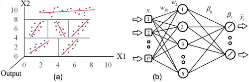
where x_k stands for the input value; y_i is the MLPNN output (i = 1, 2, …, number of targets); F is the transfer function (usually sigmoidal for the hidden layer(s) and linear for the output layer); p and q are the number of elements for the input vector and the number of neurons in the hidden layer(s), respectively; w and $\beta$ are the synaptic weights; and b is the bias.

After establishing an ANN, the network must be trained. To this end, many optimization algorithms can be utilized. The present study employed the Levenberg-Marquardt (LM) algorithm to update network weights. The LM algorithm (which is also known as the damped least-squares method) is an iterative technique which can be applied for searching local minima of complex functions. Detailed information about the LM algorithm can be found in several references (e.g. Kumar et al. 2002).

2.5 Performance indicators

Following the literature on the validation of predictive models, the models in this research are validated using various statistical indicators (Sanikhani et al. 2018, Kisi and Yaseen 2019). The models are evaluated with respect to mean absolute error (MAE), root mean square error (RMSE), agreement index (d) and Nash-Sutcliffe efficiency (NSE), which may be calculated using the following equations:

(11) $\mathrm{M}\mathrm{A}\mathrm{E}=\frac{1}{N}\sum _{i=1}^N\left|{(\mathrm{E}{\mathrm{T}}_0)}_i-{(\mathrm{E}{\mathrm{T}}_p)}_i\right|$(11)

(12) $\mathrm{R}\mathrm{M}\mathrm{S}\mathrm{E}=\sqrt{\frac{1}{N}\sum _{i=1}^N{[{(\mathrm{E}{\mathrm{T}}_0)}_i-{(\mathrm{E}{\mathrm{T}}_p)}_i]}^2}$(12)

(13) $d=1-\frac{\sum _{i=1}^N{[{(\mathrm{E}{\mathrm{T}}_0)}_i-{(\mathrm{E}{\mathrm{T}}_p)}_i]}^2}{\sum _{i=1}^N{[\left|{(\mathrm{E}{\mathrm{T}}_0)}_i-{\overline{\mathrm{E}\mathrm{T}}}_0\left|+\right|{(\mathrm{E}{\mathrm{T}}_p)}_i-{\overline{\mathrm{E}\mathrm{T}}}_0\right|]}^2},0<d\le 1$(13)

(14) $\mathrm{N}SE=1-\frac{\sum _{i=1}^N{[{(\mathrm{E}{\mathrm{T}}_0)}_i-{(\mathrm{E}{\mathrm{T}}_p)}_i]}^2}{\sum _{i=1}^N{[{(\mathrm{E}{\mathrm{T}}_0)}_i-{\overline{\mathrm{E}\mathrm{T}}}_0]}^2},-\mathrm{\infty }<\mathrm{N}SE\le 1$(14)

where N is the number of data; and ET₀, ET_p and ${\overline{\mathrm{E}\mathrm{T}}}_0$ are, respectively, the observed, predicted and mean of observed reference evapotranspiration. When MAE and RMSE values tend to zero, the predicted data obtained using the model indicate perfect performance. A perfect fitness of the predicted data with observed ET₀ is given when d = 1 or NSE = 1. These evaluation metrics were selected in this study because they are commonly used in the related literature (Shamshirband et al. 2015, Petković et al. 2016, Khoshravesh et al. 2017, Keshtegar et al. 2018a).

3 Case study

Daily climatic data of air temperature (T), solar radiation (SR), relative humidity (RH) and wind speed (W) were obtained from the stations Isparta (37°47′N, 30°34′E; altitude: 997 m a.m.s.l.) and Antalya (36°42′N, 30°44′E; altitude: 47 m a.m.s.l.), located in the Mediterranean region of Turkey. The locations of the stations are shown in Figure 2. The data used were obtained from the Turkish Meteorological Organization for the data periods 1973–2002 and 1978–2002 for Antalya and Isparta, respectively, of which 60% was used for training of the applied models and the remaining 40% was used for testing the obtained models. A summary of the statistical characteristics of the datasets is provided in Table 1. The T and SR show low skewed distribution and have high correlations with ET₀, while W has significantly highly skewed distribution and low correlation, especially for Isparta station. This low correlation may be due to the high altitude of this station. It should be noted that the mean relative humidity is more than 60% for both stations. According to the correlations given in Table 1, T and SR seem to be the most effective parameters for ET₀ estimation.

Figure 2. Location of the stations in the Mediterranean region of Turkey.

Table 1. Daily statistical parameters of each dataset. x_min, x_max, x_mean, S_x and C_sx denote minimum, maximum, mean, standard deviation and skewness, respectively.

Station	Variable	xmin	xmax	xmean	Sx	Csx	Correlation with ET0
Antalya	T (°C)	1.70	37.5	18.5	7.11	0.17	0.755
	SR (MJ/m^2)	0.15	33.4	17.2	7.50	−0.23	0.828
	RH (%)	14.0	98.0	63.7	16.8	−0.45	−0.680
	W (m/s)	0	13.0	2.80	1.55	1.90	0.274
	ET0 (mm)	0	15.0	4.08	2.40	0.70	1.000
Isparta	T (°C)	−10.5	29.4	12.0	7.93	−0.09	0.821
	SR (MJ/m^2)	0.32	30.6	13.4	5.87	−0.01	0.909
	RH (%)	19.3	96.7	61.2	13.6	0.14	−0.792
	W (m/s)	0	10.9	1.94	1.33	1.48	0.072
	ET0 (mm)	0	8.19	2.67	1.67	0.36	1.000

4 Application and results

In this study, PCE, M5Tree, MLPNN and RSM were applied for estimation of ET₀. First, an effective variable was used as the only input to the models; then, other climatic variables were added one by one considering the correlation values between each of them and ET₀. Thus, the following input combinations were tried: (i) T, (ii) T and SR, (iii) T, SR and RH, and (iv) T, SR, RH and W. This strategy was also used in previous research (e.g. Doğan 2009, Tabari et al. 2010, Cobaner 2011, Ladlani et al. 2012, Citakoglu et al. 2014, Yang et al. 2017a).

The models for the simulation of ET₀ in the training period for Isparta and Antalya stations are compared in Tables 2 and 3, respectively. It is apparent from Tables 2 and 3 that each method shows different training performance for different input combinations. At Isparta station, with input combinations (i)–(iii), the M5Tree has the best approximation, while the PCE has the best accuracy with input combination (iv). The PCE has the second-best approximation with input combination (iii), while the MLPNN is the second most accurate with the other three input combinations. The RSM generally has the worst performance in approximation of ET₀ for Isparta station. For Antalya station, the M5Tree has better approximation than the other methods for input combinations (i)–(iii), while the PCE has the best accuracy with combination (iv). The performance of the MLPNN is in the second rank for three combinations, while the RSM generally has the worst approximation of ET₀ estimation at Antalya station. It is clear from Tables 2 and 3 that the accuracy of the models in training is increased by adding a new variable as input, and the four-input models gave the best approximation. The PCE had the smallest MAE (0.038 and 0.033 mm) and RMSE (0.053 and 0.046 mm), and the highest d (0.9997 and 0.9999) and NSE (0.9990 and 0.9996) in the training period for Isparta and Antalya stations, respectively.

Table 2. Comparison of statistical errors for PCE, RSM, M5Tree and MLPNN models for estimation of ET₀ in the training stage – Isparta station.

Input variable(s)	Model	MAE (mm)	RMSE (mm)	d	NSE	Max(Re) (%)	Min(Re) (%)	d/RMSE
T	PCE	0.698	0.882	0.9127	0.7193	4.364	−3.455	1.035
	M5Tree	0.682	0.871	0.9154	0.7264	4.288	−3.407	1.051
	MLPNN	0.692	0.878	0.9136	0.7218	4.358	−3.454	1.040
	RSM	0.723	0.903	0.9072	0.7060	4.555	−3.262	1.005
T, SR	PCE	0.329	0.453	0.9804	0.9259	3.715	−1.106	2.164
	M5Tree	0.219	0.336	0.9895	0.9593	2.785	−1.700	2.944
	MLPNN	0.329	0.451	0.9805	0.9267	3.713	−1.194	2.174
	RSM	0.333	0.457	0.9801	0.9248	3.749	−1.056	2.146
T, SR, RH	PCE	0.263	0.365	0.9875	0.9519	2.544	−1.476	2.705
	M5Tree	0.136	0.221	0.9955	0.9824	1.835	−1.922	4.505
	MLPNN	0.273	0.375	0.9867	0.9492	2.664	−1.230	2.629
	RSM	0.269	0.372	0.9871	0.9501	2.678	−1.333	2.654
T, SR, RH, W	PCE	0.038	0.053	0.9997	0.9990	0.362	−0.252	18.963
	M5Tree	0.047	0.065	0.9996	0.9985	0.610	−0.335	15.401
	MLPNN	0.047	0.063	0.9996	0.9986	0.441	−0.495	15.891
	RSM	0.062	0.087	0.9993	0.9973	0.716	−0.435	11.474

Table 3. Comparison of statistical errors for PCE, RSM, M5Tree and MLPNN models for estimation of ET₀ in the training stage – Antalya station.

Input variable(s)	Model	MAE (mm)	RMSE (mm)	d	NSE	Max(Re) (%)	Min(Re) (%)	d/RMSE
T	PCE	1.152	1.436	0.8754	0.6291	6.425	−4.188	0.760
	M5Tree	1.107	1.401	0.8832	0.6472	6.030	−4.064	0.798
	MLPNN	1.135	1.426	0.8766	0.6346	6.232	−4.268	0.773
	RSM	1.153	1.436	0.8753	0.6290	6.411	−4.162	0.759
T, SR	PCE	0.744	1.004	0.9480	0.8188	6.109	−2.936	1.275
	M5Tree	0.444	0.690	0.9772	0.9145	5.126	−3.482	2.200
	MLPNN	0.733	0.993	0.9491	0.8225	6.171	−2.534	1.295
	RSM	0.765	1.032	0.9446	0.8085	5.848	−2.724	1.235
T, SR, RH	PCE	0.247	0.399	0.9927	0.9714	2.937	−3.770	4.024
	M5Tree	0.145	0.257	0.9970	0.9881	2.438	−2.698	6.893
	MLPNN	0.245	0.397	0.9928	0.9717	3.034	−4.196	4.057
	RSM	0.253	0.405	0.9924	0.9705	2.950	−3.708	3.918
T, SR, RH, W	PCE	0.033	0.046	0.9999	0.9996	0.371	−0.185	30.671
	M5Tree	0.051	0.076	0.9997	0.9990	0.625	−0.731	19.537
	MLPNN	0.055	0.080	0.9997	0.9989	0.825	−0.558	18.103
	RSM	0.066	0.097	0.9996	0.9983	0.866	−0.690	15.248

The performance statistics of the four models applied in the estimation of ET₀ for Isparta station in the test stage are presented in Table 4. As seen from Table 4, the PCE has a better accuracy than the other three models for input combinations (iii) and (iv), while the MLPNN and RSM have the best accuracy with combinations (i) and (ii), respectively. In fact, there is a slight difference between the MLPNN and PCE for the first input combination. In the test period, the M5Treee generally has the worst accuracy in estimating ET₀ at Isparta station. Similar to the training period, the performance of the models increased by including more inputs; the four-input models have the best accuracy. The PCE model has the lowest MAE (0.036 mm) and RMSE (0.047), and the highest d (0.9998) and NSE (0.9992) in estimating ET₀ for Isparta station.

Table 4. Comparison of statistical errors for PCE, RSM, M5Tree and MLPNN models for estimation of ET₀ in the test stage – Isparta station.

Input variable(s)	Model	MAE (mm)	RMSE (mm)	d	NSE	max(RE)^#	Mean* (mm)	SD* (mm)	Total SR* (mm)
T	PCE	0.782	0.970	0.8991	0.6662	3.221	2.911	1.464	7609.289
	M5Tree	0.783	0.976	0.8978	0.6616	3.208	2.907	1.466	7599.913
	MLPNN	0.779	0.968	0.8988	0.6677	3.247	2.903	1.454	7588.014
	RSM	0.801	0.993	0.8962	0.6497	3.653	2.948	1.504	7704.991
T, SR	PCE	0.509	0.656	0.9668	0.8471	2.694	3.079	1.925	8048.136
	M5Tree	0.508	0.670	0.9638	0.8405	3.075	3.030	1.859	7920.428
	MLPNN	0.544	0.722	0.9609	0.8150	2.903	3.117	1.972	8147.602
	RSM	0.498	0.623	0.9695	0.8623	2.341	3.065	1.889	8012.054
T, SR, RH	PCE	0.330	0.437	0.9840	0.9322	2.061	2.885	1.782	7540.156
	M5Tree	0.381	0.517	0.9766	0.9050	2.666	2.860	1.731	7477.123
	MLPNN	0.353	0.454	0.9828	0.9267	1.870	2.925	1.794	7645.583
	RSM	0.346	0.450	0.9833	0.9280	1.829	2.912	1.817	7612.744
T, SR, RH, W	PCE	0.036	0.047	0.9998	0.9992	0.206	2.675	1.679	6991.659
	M5Tree	0.075	0.134	0.9984	0.9937	1.638	2.678	1.691	7001.311
	MLPNN	0.051	0.071	0.9996	0.9982	0.633	2.667	1.679	6972.383
	RSM	0.068	0.095	0.9992	0.9968	0.625	2.680	1.704	7005.656

^# The maximum absolute relative error between the predicted and observed data is calculated as:

max(RE) = max{|(Oi − Pi)/Oi| × 100}

* Mean observed ET₀ is 2.662 mm; SD of observed ET₀ is 1.678 mm; and total observed ET₀ is 6958.53 mm, in the test stage.

The performance of the applied methods in estimation of ET₀ on the test data of Antalya station is presented in Table 5. From Table 5, it is apparent that the PCE has better estimation accuracy than the other methods for two of the four combinations, (i) and (iv), while the MLPNN has the best accuracy for input combination (ii), followed by the PCE model. With input combination (iii), both PCE and MLPNN have almost the same accuracy in estimation of ET₀ for Antalya station. Similar to the Isparta station, here also the M5Tree generally has the worst estimates. An increment in the accuracy of the models is clearly seen when the number of inputs is increased. For Antalya station also, the PCE has the lowest MAE (0.037 mm) and RMSE (0.050) and the highest d (0.9999) and NSE (0.9996) in estimating ET₀.

Table 5. Comparison of statistical errors for PCE, RSM, M5Tree and MLPNN models for estimation of ET₀ in the test stage – Antalya station.

Input variable(s)	Model	MAE (mm)	RMSE (mm)	d	NSE	max(RE)^#	Mean* (mm)	SD* (mm)	Total SR* (mm)
T	PCE	1.260	1.577	0.8710	0.5899	8.247	4.574	2.127	10 624.865
	M5Tree	1.270	1.603	0.8666	0.5766	8.227	4.583	2.136	10 646.454
	MLPNN	1.254	1.583	0.8692	0.5869	8.417	4.575	2.117	10 628.588
	RSM	1.263	1.581	0.8709	0.5882	8.257	4.578	2.137	10 634.296
T, SR	PCE	0.852	1.134	0.9453	0.7882	6.119	4.470	2.490	10 383.748
	M5Tree	0.979	1.356	0.9252	0.6970	6.900	4.496	2.633	10 444.254
	MLPNN	0.837	1.122	0.9451	0.7925	6.411	4.461	2.435	10 363.862
	RSM	0.857	1.154	0.9411	0.7807	7.028	4.433	2.405	10 298.119
T, SR, RH	PCE	0.311	0.481	0.9903	0.9619	3.039	4.439	2.441	10 312.763
	M5Tree	0.380	0.610	0.9842	0.9386	3.995	4.421	2.424	10 269.435
	MLPNN	0.310	0.481	0.9903	0.9619	3.325	4.436	2.428	10 305.185
	RSM	0.311	0.486	0.9901	0.9611	3.218	4.429	2.429	10 287.652
T, SR, RH, W	PCE	0.037	0.050	0.9999	0.9996	0.416	4.348	2.475	10 100.223
	M5Tree	0.065	0.111	0.9995	0.9980	2.093	4.348	2.475	10 099.855
	MLPNN	0.066	0.099	0.9996	0.9984	1.240	4.361	2.459	10 130.176
	RSM	0.074	0.109	0.9995	0.9981	0.725	4.351	2.478	10 106.393

^# The maximum absolute relative error between the predicted and observed data, calculated as:

max(RE) = max{|(Oi − Pi)/Oi| × 100}

* Mean observed ET₀ is 4.329 mm; SD of observed ET₀ is 2.463 mm; and total observed ET₀ is 10,056.39 mm, in the test stage.

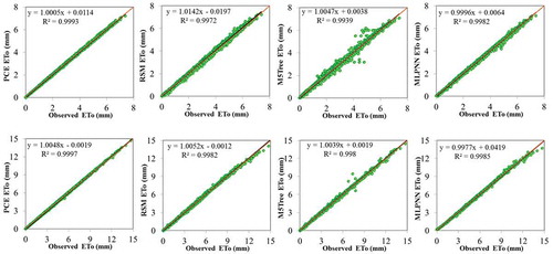
The observed and estimated ET₀ values are compared for each method and each combination in Figures 3–6. It is clear from these scatter plots that including more variables in the model inputs results in less scattered estimates for both stations. It may be seen from Figures 3–6 that the estimates of the four-input models are closer to the observed ET₀ than those of the other models that use different input combinations; the four-input PCE has less scattered estimates compared to the corresponding M5Tree, MLPNN and RSM models. Comparison of Figures 5 and 6 indicates that adding wind speed input considerably improved the accuracy of the models in estimation of ET₀ at both stations, even though this parameter has the lowest correlation with ET₀ (see Table 1). This implies that there is a strong nonlinear relationship between the W and ET₀. The comparison of the two stations suggests that the models are better in estimating ET₀ for Antalya compared to Isparta. The main reason for this might be the difference in altitude and climatic characteristics of these locations. This can be clearly seen from the temperature ranges shown in Table 1: the temperature at Antalya is in the range [1.7, 37.5], while that at Isparta is [−10.5, 29.5]. Similarly, the ET₀ ranges are [0, 15] and [0, 8.19] for Antalya and Isparta, respectively.

Figure 3. Scatter plots of observed and different estimated ET₀ models for Isparta station (top row) and Antalya station (bottom row) in the test period based on the input variable mean air temperature.

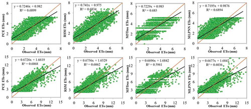
Figure 4. Scatter plots of observed and different estimated ET₀ models for Isparta station (top row) and Antalya station (bottom row) in the test period based on the input variables mean air temperature and solar radiation.

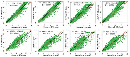
Figure 5. Scatter plots of observed and different estimated ET₀ models for Isparta station (top row) and Antalya station (bottom row) in the test period based on the input variables mean air temperature, solar radiation and mean relative humidity.

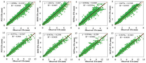
Figure 6. Scatter plots of observed and different estimated ET₀ models for Isparta station (top row) and Antalya station (bottom row) in the test period based on the input variables mean air temperature, solar radiation, mean relative humidity and wind speed.

5 Conclusion

This study investigated the ability of a new method, polynomial chaos expansion (PCE), to model reference evapotranspiration. The results of the PCE were compared with those of the M5 model tree (M5Tree), the multi-layer perceptron neural network (MLPNN), and the response surface method (RSM) with respect to various evaluation criteria. Daily climatic data from two stations situated in the Mediterranean region of Turkey were used as case studies. Application of various combinations of input data indicated that the four-input models, comprising temperature, solar radiation, relative humidity and wind speed as inputs, have the best accuracy in predicting ET₀. From the comparison of the four methods, the PCE provided the best accuracy in modelling ET₀ followed by the MLPNN, RSM and M5Tree, respectively. The addition of wind speed as input in the models increased the models’ accuracy considerably, even though wind speed has low correlation with ET₀. This indicated the importance of including wind speed for the accurate estimation of ET₀. The applied models gave better estimates for Antalya station compared to Isparta. The possible reasons for this were thought to be the differences in altitude and climatic characteristics of these two stations. The ability of PCE to predict complex engineering problems such as ET₀ should be evaluated for other stations with different climates in future studies.

Disclosure statement

No potential conflict of interest was reported by the authors.

References

- Allen, R.G., 2000. Using the FAO-56 dual crop coefficient method over an irrigated region as part of an evapotranspiration intercomparison study. Journal of Hydrology, 229 (1–2), 27–41. doi:10.1016/S0022-1694(99)00194-8.
- Beeson, R., 2006. Relationship of plant growth and actual evapotranspiration to irrigation frequency based on management allowed deficits for container nursery stock. Journal of the American Society for Horticultural Science, 131 (1), 140–148. doi:10.21273/JASHS.131.1.140.
- Blatman, G. and Sudret, B., 2010. An adaptive algorithm to build up sparse polynomial chaos expansions for stochastic finite element analysis. Probabilistic Engineering Mechanics, 25 (2), 183–197. doi:10.1016/j.probengmech.2009.10.003.
- Citakoglu, H., et al., 2014. Estimation of monthly mean reference evapotranspiration in Turkey. Water Resources Management, 28 (1), 99–113. doi:10.1007/s11269-013-0474-1.
- Cobaner, M., 2011. Evapotranspiration estimation by two different neuro-fuzzy inference systems. Journal of Hydrology, 398 (3–4), 292–302. doi:10.1016/j.jhydrol.2010.12.030.
- Doğan, E., 2009. Reference evapotranspiration estimation using adaptive neuro‐fuzzy inference systems. Irrigation and Drainage: the Journal of the International Commission on Irrigation and Drainage, 58 (5), 617–628. doi:10.1002/ird.445.
- Fajraoui, N., et al., 2011. Use of global sensitivity analysis and polynomial chaos expansion for interpretation of nonreactive transport experiments in laboratory‐scale porous media. Water Resources Research, 47 (2). doi:10.1029/2010WR009639.
- Feng, Y., et al., 2017. Modeling reference evapotranspiration using extreme learning machine and generalized regression neural network only with temperature data. Computers and Electronics in Agriculture, 136, 71–78. doi:10.1016/j.compag.2017.01.027
- Gavili, S., et al., 2018. Evaluation of several soft computing methods in monthly evapotranspiration modelling. Meteorological Applications, 25 (1), 128–138. doi:10.1002/met.2018.25.issue-1.
- George, B.A., et al., 2002. Decision support system for estimating reference evapotranspiration. Journal of Irrigation and Drainage Engineering, 128 (1), 1–10. doi:10.1061/(ASCE)0733-9437(2002)128:1(1).
- Gocic, M., et al., 2016. Comparative analysis of reference evapotranspiration equations modelling by extreme learning machine. Computers and Electronics in Agriculture, 127, 56–63. doi:10.1016/j.compag.2016.05.017
- Keshtegar, B., et al., 2016. Optimized river stream-flow forecasting model utilizing high-order response surface method. Water Resources Management, 30 (11), 3899–3914. doi:10.1007/s11269-016-1397-4.
- Keshtegar, B., et al., 2018a. Subset modeling basis ANFIS for prediction of the reference evapotranspiration. Water Resources Management, 32 (3), 1101–1116. doi:10.1007/s11269-017-1857-5.
- Keshtegar, B., et al., 2019. A novel nonlinear modeling for the prediction of blast-induced airblast using a modified conjugate FR method. Measurement, 131, 35–41. doi:10.1016/j.measurement.2018.08.052
- Keshtegar, B. and Heddam, S., 2017. Modeling daily dissolved oxygen concentration using modified response surface method and artificial neural network: a comparative study. Neural Computing and Applications. doi:10.1007/s00521-017-2917-8.
- Keshtegar, B. and Kisi, O., 2017. Modified response-surface method: new approach for modeling pan evaporation. Journal of Hydrologic Engineering, 22 (10), 04017045. doi:10.1061/(ASCE)HE.1943-5584.0001541.
- Keshtegar, B., Mert, C., and Kisi, O., 2018b. Comparison of four heuristic regression techniques in solar radiation modeling: kriging method vs RSM, MARS and M5 model tree. Renewable and Sustainable Energy Reviews, 81, 330–341. doi:10.1016/j.rser.2017.07.054
- Khoshravesh, M., Sefidkouhi, M.A.G., and Valipour, M., 2017. Estimation of reference evapotranspiration using multivariate fractional polynomial, Bayesian regression, and robust regression models in three arid environments. Applied Water Science, 7 (4), 1911–1922. doi:10.1007/s13201-015-0368-x.
- Kim, S., et al., 2014. Modeling nonlinear monthly evapotranspiration using soft computing and data reconstruction techniques. Water Resources Management, 28 (1), 185–206. doi:10.1007/s11269-013-0479-9.
- Kisi, Ö., 2006. Generalized regression neural networks for evapotranspiration modelling. Hydrological Sciences Journal, 51 (6), 1092–1105. doi:10.1623/hysj.51.6.1092.
- Kisi, O., 2013. Least squares support vector machine for modeling daily reference evapotranspiration. Irrigation Science, 31 (4), 611–619. doi:10.1007/s00271-012-0336-2.
- Kisi, O., et al., 2015. Long-term monthly evapotranspiration modeling by several data-driven methods without climatic data. Computers and Electronics in Agriculture, 115, 66–77. doi:10.1016/j.compag.2015.04.015
- Kisi, O., 2015. Pan evaporation modeling using least square support vector machine, multivariate adaptive regression splines and M5 model tree. Journal of Hydrology, 528, 312–320. doi:10.1016/j.jhydrol.2015.06.052
- Kisi, O., et al., 2016. Daily pan evaporation modeling using chi-squared automatic interaction detector, neural networks, classification and regression tree. Computers and Electronics in Agriculture, 122, 112–117. doi:10.1016/j.compag.2016.01.026
- Kisi, O., 2016. Modeling reference evapotranspiration using three different heuristic regression approaches. Agricultural Water Management, 169, 162–172. doi:10.1016/j.agwat.2016.02.026
- Kisi, O. and Kilic, Y., 2016. An investigation on generalization ability of artificial neural networks and M5 model tree in modeling reference evapotranspiration. Theoretical and Applied Climatology, 126 (3–4), 413–425. doi:10.1007/s00704-015-1582-z.
- Kisi, O. and Yaseen, Z.M., 2019. The potential of hybrid evolutionary fuzzy intelligence model for suspended sediment concentration prediction. CATENA, 174, 11–23. doi:10.1016/j.catena.2018.10.047
- Kisi, O. and Zounemat-Kermani, M., 2014. Comparison of two different adaptive neuro-fuzzy inference systems in modelling daily reference evapotranspiration. Water Resources Management, 28 (9), 2655–2675. doi:10.1007/s11269-014-0632-0.
- Kumar, M., et al., 2002. Estimating evapotranspiration using artificial neural network. Journal of Irrigation and Drainage Engineering, 128 (4), 224–233. doi:10.1061/(ASCE)0733-9437(2002)128:4(224).
- Kumar, M., Raghuwanshi, N., and Singh, R., 2011. Artificial neural networks approach in evapotranspiration modeling: a review. Irrigation Science, 29 (1), 11–25. doi:10.1007/s00271-010-0230-8.
- Ladlani, I., et al., 2012. Modeling daily reference evapotranspiration (ET0) in the north of Algeria using generalized regression neural networks (GRNN) and radial basis function neural networks (RBFNN): a comparative study. Meteorology and Atmospheric Physics, 118 (3–4), 163–178. doi:10.1007/s00703-012-0205-9.
- Laloy, E., et al., 2013. Efficient posterior exploration of a high‐dimensional groundwater model from two‐stage Markov chain Monte Carlo simulation and polynomial chaos expansion. Water Resources Research, 49 (5), 2664–2682. doi:10.1002/wrcr.20226.
- Landeras, G., Ortiz-Barredo, A., and López, J.J., 2008. Comparison of artificial neural network models and empirical and semi-empirical equations for daily reference evapotranspiration estimation in the Basque Country (Northern Spain). Agricultural Water Management, 95 (5), 553–565. doi:10.1016/j.agwat.2007.12.011.
- Lasota, R., et al., 2015. Polynomial chaos expansion method in estimating probability distribution of rotor-shaft dynamic responses. Bulletin of the Polish Academy of Sciences Technical Sciences, 63 (2), 413–422. doi:10.1515/bpasts-2015-0047.
- Misaghian, N., et al., 2017. Predicting the reference evapotranspiration based on tensor decomposition. Theoretical and Applied Climatology, 130 (3–4), 1099–1109. doi:10.1007/s00704-016-1943-2.
- Nguyen, K.Q., et al., 2017. Artificial lights improve the catchability of snow crab (Chionoecetes opilio) traps. Aquaculture and Fisheries, 2 (3), 124–133. doi:10.1016/j.aaf.2017.05.001.
- Pal, M. and Deswal, S., 2009. M5 model tree based modelling of reference evapotranspiration. Hydrological Processes, 23 (10), 1437–1443. doi:10.1002/hyp.v23:10.
- Petković, D., et al., 2015. Determination of the most influential weather parameters on reference evapotranspiration by adaptive neuro-fuzzy methodology. Computers and Electronics in Agriculture, 114, 277–284. doi:10.1016/j.compag.2015.04.012.
- Petković, D., et al., 2016. Particle swarm optimization-based radial basis function network for estimation of reference evapotranspiration. Theoretical and Applied Climatology, 125 (3–4), 555–563. doi:10.1007/s00704-015-1522-y.
- Quinlan, J.R., 1992. Learning with continuous classes. In: 5th Australian joint conference on artificial intelligence, Singapore, 343–348.
- Sanikhani, H., et al., 2018. Temperature-based modeling of reference evapotranspiration using several artificial intelligence models: application of different modeling scenarios. Theoretical and Applied Climatology. doi:10.1007/s00704-018-2390-z.
- Sattari, M.T., et al., 2013. M5 model tree application in daily river flow forecasting in Sohu Stream, Turkey. Water Resources, 40 (3), 233–242. doi:10.1134/S0097807813030123.
- Shamshirband, S., et al., 2015. Estimation of reference evapotranspiration using neural networks and cuckoo search algorithm. Journal of Irrigation and Drainage Engineering, 142 (2), 04015044. doi:10.1061/(ASCE)IR.1943-4774.0000949.
- Sochala, P. and Le Maître, O., 2013. Polynomial Chaos expansion for subsurface flows with uncertain soil parameters. Advances in Water Resources, 62, 139–154. doi:10.1016/j.advwatres.2013.10.003
- Tabari, H., Marofi, S., and Sabziparvar, -A.-A., 2010. Estimation of daily pan evaporation using artificial neural network and multivariate non-linear regression. Irrigation Science, 28 (5), 399–406. doi:10.1007/s00271-009-0201-0.
- Wang, L., et al., 2017a. Evaporation modelling using different machine learning techniques. International Journal of Climatology, 37, 1076–1092. doi:10.1002/joc.2017.37.issue-S1.
- Wang, L., et al., 2017b. Influence of main-panel angle on the hydrodynamic performance of a single-slotted cambered otter-board. Aquaculture and Fisheries, 2 (5), 234–240. doi:10.1016/j.aaf.2017.09.001.
- Wang, L., et al., 2017c. Pan evaporation modeling using six different heuristic computing methods in different climates of China. Journal of Hydrology, 544, 407–427. doi:10.1016/j.jhydrol.2016.11.059
- Wang, L., et al., 2017d. Pan evaporation modeling using four different heuristic approaches. Computers and Electronics in Agriculture, 140, 203–213. doi:10.1016/j.compag.2017.05.036
- Wang, S., et al., 2015. A polynomial chaos ensemble hydrologic prediction system for efficient parameter inference and robust uncertainty assessment. Journal of Hydrology, 530, 716–733. doi:10.1016/j.jhydrol.2015.10.021
- Wen, X., et al., 2015. Support-vector-machine-based models for modeling daily reference evapotranspiration with limited climatic data in extreme arid regions. Water Resources Management, 29 (9), 3195–3209. doi:10.1007/s11269-015-0990-2.
- Wiener, N., 1938. The homogeneous chaos. American Journal of Mathematics, 60 (4), 897–936. doi:10.2307/2371268.
- Xiu, D. and Karniadakis, G.E., 2002. The Wiener–askey polynomial chaos for stochastic differential equations. SIAM Journal on Scientific Computing, 24 (2), 619–644. doi:10.1137/S1064827501387826.
- Yang, G., et al., 2017a. Effect of the exposure to suspended solids on the enzymatic activity in the bivalve Sinonovacula constricta. Aquaculture and Fisheries, 2 (1), 10–17. doi:10.1016/j.aaf.2017.01.001.
- Yang, Y., Liu, Z., and Liu, Y., 2017b. Prediction of lute acoustic quality based on soundboard vibration performance using multiple choice model. Journal of Forestry Research, 28 (4), 855–861. doi:10.1007/s11676-016-0365-4.
- Yaseen, Z.M., et al., 2018. Application of the hybrid artificial neural network coupled with rolling mechanism and grey model algorithms for streamflow forecasting over multiple time horizons. Water Resources Management, 32 (5), 1883–1899. doi:10.1007/s11269-018-1909-5.
- Yin, Z., et al., 2017. Integrating genetic algorithm and support vector machine for modeling daily reference evapotranspiration in a semi-arid mountain area. Hydrology Research, 48 (5), 1177–1191. doi:10.2166/nh.2016.205.
- Zanetti, S., et al., 2007. Estimating evapotranspiration using artificial neural network and minimum climatological data. Journal of Irrigation and Drainage Engineering, 133 (2), 83–89. doi:10.1061/(ASCE)0733-9437(2007)133:2(83).