A two-stage sensitivity analysis for parameter identification and calibration of a physically-based distributed model in a river basin

ABSTRACT

Hydrological models demand large numbers of input parameters, which are to be optimally identified for better simulation of various hydrological processes. Identifying the most relevant parameters and their values using efficient sensitivity analysis methods helps to better understand model performance. In this study, the physically-based distributed model SHETRAN is used for hydrological simulation on the Netravathi River Basin in south India and the most important parameters are identified using the Morris screening method. Further, the influence of a particular model parameter on streamflow is quantified using local sensitivity analysis and optimal parameters are obtained for calibration of the SHETRAN model. The results demonstrate the capability of two-stage sensitivity analysis, combining qualitative and quantitative methods in the initial screening-out of insignificant model parameters, identifying parameter interactions and quantifying the contribution of each model parameter to the streamflow. The results of the sensitivity analysis simplified the calibration procedure of SHETRAN for the study area.

KEYWORDS:

• hydrological simulation
• distributed model
• sensitivity analysis
• SHETRAN
• Morris analysis
• calibration

Editor A. Castellarin Associate editor A. Petroselli

1 Introduction

Physically-based, spatially-distributed models are utilized to an increasing extent for assessing the effects of future climate and land-use changes at the river basin scale (Bovolo et al. 2009, Birkinshaw et al. 2011, Mourato et al. 2015). Distributed models represent the spatial heterogeneity of hydrological processes within a river basin more realistically. However, the complexity of these models demands the determination of a multitude of parameters (Muleta and Nicklow 2005), the values of which may not be directly measurable in the field (Brazier et al. 2000, Wagener 2003, Benke et al. 2008). Unaffordable cost, experimental constraints, or the scaling problem are major hurdles that prevent direct access to the parameters from the catchment data (Beven et al. 1980). Therefore, model calibration is an essential step in reducing the effect of uncertainty of parameters on simulation results (Cibin et al. 2010).

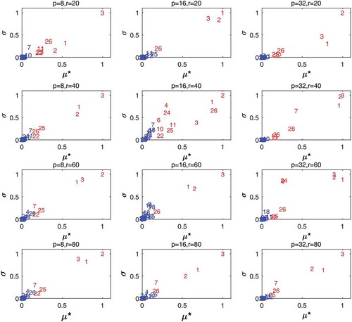
Figure 6. Sensitivity analysis results of Morris screening using different r and p for objective function RMSE. Numbers in red are supposed to be sensitive parameters. The closer the parameter is to the upper right, the more sensitive it is.

The high computational effort, parameter spaces displaying high interaction, and nonlinear and multi-model objective spaces make the calibration of highly parameterized models difficult (Gupta et al. 1998, Carpenter et al. 2001). Insufficient knowledge regarding model parameter sensitivities directs modellers to focus on insensitive parameters, which is futile (Bahremand and De Smedt 2008). Hence, emphasis on sensitive parameters can provide a better understanding of the model and result in better simulations with reduced uncertainty (Lenhart et al. 2002). Therefore, sensitivity analysis (SA) acts as an important tool to identify and rank parameters that exhibit a significant impact on specific model outputs of interest (Saltelli et al. 2000, Sieber and Uhlenbrook 2005, Herman et al. 2013). The reduction in dimensionality of parameter space by performing sensitivity analysis speeds the model calibration and validation, and helps in prioritization of efforts for uncertainty reduction (Demaria et al. 2007, Norton 2015). The model calibration time can be reduced by concentrating estimation efforts on the most significant model parameters for predictions identified using parameter SA (Rakovec et al. 2014, Ye et al. 2014). Therefore, it would be a good option to apply SA methods prior to the model calibration of distributed hydrological models having numerous parameters.

The SA methods may be broadly classified into local and global (van Griensven et al. 2006). Local SA methods determine the model response by individually changing the input parameters while maintaining nominal values for the other parameters (Spruill et al. 2000, Holvoet et al. 2005). Applications of local SA, or the one-at-a-time (OAT) method, owing to the simplicity of the method, may be found in various hydrological models. However, the linear relationship assumed between the parameter and the model output is a major limitation of the OAT method, which makes its application to complex and nonlinear models unreliable (Wagener and Kollat 2007). In contrast, global SA (GSA) methods determine the effect of variations in input on the output by considering the entire parameter space and possible parameter interactions (Tarantola et al. 2002, Tong 2010, Sarrazin et al. 2016). Due to high computational demands for sampling the parameter space, GSA application on spatially-distributed models is limited. However, in recent years, modellers have applied GSA on an entire set of spatially-distributed parameters (e.g. Tang et al. 2007, Van Werkhoven et al. 2008, Pan et al. 2017). Some of the common global sensitivity analysis methods that have been applied to different hydrological models are: (a) regional sensitivity analysis (RSA; Hornberger and Spear 1981) applied to the conceptual HBV model (Abebe et al. 2010, Zelelew and Alfredsen 2013) and the VIC model (Demaria et al. 2007); (b) variance-based methods (Sobol‘ 1993) applied to the HL-RDHM model (Tang et al. 2007) and the SWAT model (Nossent et al. 2011, Zhang et al. 2013a); and (c) Latin hypercube OAT applied to the SWAT model (Holvoet et al. 2005, van Griensven et al. 2006). The Morris method ranks the input parameters according to their order of significance and provides sensitivity measures qualitatively (Morris 1991). The method has been applied to different hydrological models (Matthews et al. 2007, Kelleher et al. 2015, Osuch et al. 2015) as an initial step of global sensitivity analysis.

The SHETRAN model (see Section 2.3) has been widely applied to simulate water and sediment discharge (Bathurst et al. 2006, Elliott et al. 2012), as well as to study the impact of climate and land-use change (Bathurst et al. 2004, Azim et al. 2016, Birkinshaw et al. 2016). SHETRAN is a physically-based, distributed model characterized by a large number of input parameters. The effective manual calibration of physically-based distributed models can be achieved only through rigorous and purposeful parameterization (Refsgaard 1997). Generally, the key calibration parameters of the SHETRAN model are adjusted according to physical reasoning for manual calibration (Birkinshaw et al. 2011), or automatically using the Shuffled Complex Evolution algorithm (Zhang et al. 2013b). Manual calibration becomes a tedious procedure in river basins that are highly heterogeneous in terms of environmental conditions. And the SHETRAN model lacks modules for sensitivity analysis and calibration. Hence, previous studies of sensitivity analysis performed on SHETRAN were limited to local SA or ranking based on multi-model responses; these SA methods were inadequate in representing the model parameter interactions. Anderton et al. (2002) used an approach similar to the GLUE method of Beven and Binley (1992) by ranking subsurface flow parameters in SHETRAN considering multiple model responses. Their study revealed the complex model parameter interactions in SHETRAN and noted that the sensitivity of individual parameters changed according to other parameter values. Đukić and Radić (2016) quantified the effect of variation in SHETRAN model parameters on runoff and sediment concentration of a torrential catchment using local SA. Their study on a river catchment in Serbia identified the most sensitive model parameters for runoff as vertical saturated hydraulic conductivity, horizontal saturated hydraulic conductivity and Strickler overland coefficient. An integrated technique, wherein the qualitative and quantitative SA methods are combined, helps to reduce the high computational demands of GSA methods applied in complex hydrological models (Francos et al. 2003, Yang 2011, Sun et al. 2012).

This paper implements a two-stage sensitivity approach consisting of two methods of SA, namely the Morris method (Morris 1991) and a local SA method, applied to the SHETRAN model parameters, with a case study of a humid tropical river basin, the Netravathi in India. The effectiveness of the Morris method as a tool to handle the high-dimensional parameter space of the SHETRAN model is evaluated. The parameters are ranked qualitatively, followed by screening-out of the unimportant ones in the first stage, with relatively small computational cost. In the second stage, the sensitivity of the relevant parameters is quantified using local sensitivity. The main focus of this paper is to demonstrate the capability of the two-stage SA method to reduce the high-dimensional parameter space of the SHETRAN model for successful manual calibration based on the case study of the Netravathi River Basin.

2 Materials and methods

2.1 Study area

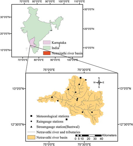
The Netravathi River Basin, located at 12°30′–13°10′N and 74°50′–75°50′E (Fig. 1), is selected as the study area. The Netravathi River is an important west-flowing river in Karnataka, India. The river originates in the Western Ghats region (a mountain range running along the western edge of the Deccan Plateau in South India, which is identified as one of the 25 hotspots for bio-diversity conservation in the world) at Gangamoola near Samse village, and flows westward to discharge into the Arabian Sea. The river has a total length of 103 km and drains an area of 3657 km² (Central Water Commission 2006). The altitude of the basin varies from 0 to 1860 m a.s.l. The climate of the basin is characterized by heavy rainfall, high humidity and oppressive weather in the hot season. The average annual rainfall over the basin is 3930 mm; the mean daily temperature drops below 20°C during the southwest monsoon (June–September) and during the months of March–May it reaches up to 35°C.

Figure 1. Location map of Netravathi River Basin, India, and the gauging stations.

The basin receives a major part of its rainfall during the southwest monsoon, during which period the mean humidity exceeds 85%. The Netravathi River supplies water throughout the year for drinking and irrigation to a large population, and industries established in Mangalore city, as well as benefitting places of religious importance, such as Dharmastala and Kukkesubramanya (Babar and Ramesh 2015). The upper portion of the basin is covered by forest, while paddy crops cover the low-lying areas around the coastal region. In some areas, rubber plantations have been established by clearing the forests. The main crops in the highlands are coffee, tea, cardamom and other spices.

2.2 Data used

The rainfall dataset pertaining to the study area was procured from the Directorate of Economics and statistics, Karnataka, for the period from 1979 to 2010. The temperature data were collected at two stations maintained by the India Meteorological Department (IMD) for the same period (1979–2010) as the rainfall data. The potential evapotranspiration was calculated with the Blaney-Criddle equation (Blaney and Criddle 1950). The daily discharge data (1979–2010) at Bantwal station maintained by the Central Water Commission were used for calibration and validation. Figure 1 shows the locations of the raingauges, meteorological station and streamgauge station within the basin. Digital elevation model (DEM) data were extracted from the ASTER 30-m grid resolution dataset (http://earthexplorer.usgs.gov/).

The Harmonized World Soil Database (FAO 2012), at 30 arcsecond resolution, provided the required soil texture data of the topsoil (0–30 cm) and subsoil (30–100 cm) for the study region. Three soil layers of different textures were considered in this study. The bottom soil layer texture is unknown. The land-use map of Netravathi River Basin was prepared using a Landsat 5 TM image of 30 m resolution, with acquisition date of 2 January 1991. The land-use distribution is waterbody (1.9%), forest (38.4%), wasteland (0.22%), agricultural land (36.3%), grassland (19.8%) and urban area (3.28%). The maximum likelihood method, using the supervised classification technique, was used to prepare the land-use maps for the basin. The soil and land-use maps are given in the supplementary material (Fig. S1).

2.3 SHETRAN model

In this study, the hydrological model SHETRAN (http://research.ncl.ac.uk/shetran/) was utilized to perform runoff simulations for the Netravathi River Basin. SHETRAN is a physically-based, distributed model for flow, sediment and contaminant transport in river basins (Ewen et al. 2000, Birkinshaw 2010). In this model, the partial differential equations for flow and transport are solved by finite difference methods. The basin is discretized into a horizontal orthogonal river network and at each square grid in the vertical direction by a column of layers. A network of river links runs along the edges of grid squares representing the river network. The model explicitly incorporates spatial heterogeneity in topography, soil, land use and catchment properties with its grid-column structure. The model represents coupled surface/subsurface flow, allowing overland flow to be produced by rainfall excess over infiltration and by upward saturation of the soil column (Birkinshaw et al. 2011). The interception of rainfall is represented by the modified Rutter model. The actual evapotranspiration is calculated from potential evapotranspiration (PET) as a function of soil water potential. The diffusive wave approximation of the St Venant equation governs the overland and channel flow processes, while the Richards and Boussinesq equations give the one-dimensional flow in the unsaturated zone and two-dimensional flow in the saturated zone, respectively. The river–aquifer interaction is calculated using the Darcy equation.

In this study, the focus is on the calibration of the water flow component of the SHETRAN model (v 4.4.5).

2.4 Model parameterization and SHETRAN model set-up

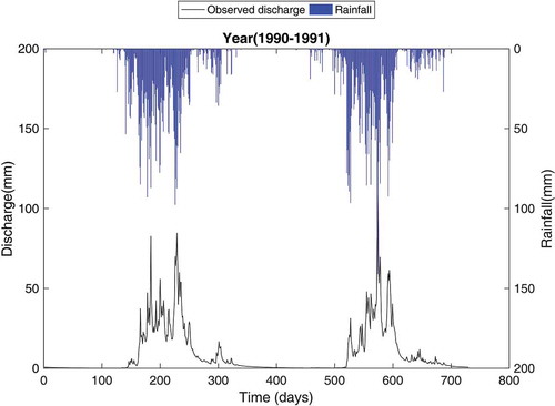
A 2 km × 2 km grid resolution was chosen for developing the SHETRAN model of the Netravathi River Basin. The catchment up to the gauging station at Bantwal is represented by 894 grid squares, with 63 river link elements representing the channel (Fig. 2). The daily rainfall and PET calculated at the stations within the basin were spatially distributed to 5 km × 5 km grids using the inverse distance weighting method for application to the SHETRAN model. The parameters deemed to affect the streamflow response were identified by a detailed literature review (Ewen and Parkin 1996, Birkinshaw et al. 2011). Daily rainfall data for the 2-year period from January 1990 to December 1991, preceded by a 1-year warm-up period, were used to force the model for sensitivity analysis (Fig. 3).

Figure 2. Elevation and the river network of Netravathi (up to Bantwal gauging station) generated in the SHETRAN model (grid resolution is 2 km × 2 km).

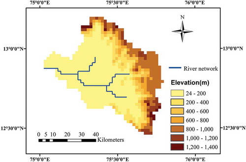
Figure 3. Observed hydrograph for Netravathi River Basin for 1990/91.

The model uses the Strickler roughness coefficient, which is the reciprocal of Manning’s roughness coefficient and is a land-use parameter. Its value was decided based on Chow (1959). Vegetation parameters in the model, consisting of maximum rooting depth, canopy storage capacity, leaf area index and AET/PET ratio, were based on the SHETRAN library. For sensitivity analysis by the Morris method and local SA, the model was run on a daily scale for the period from January 1990 to December 1991, preceded by a 1-year warm-up period. The initial sets of vectors for the computational experiments were arrived at by carrying out a random sampling of the set of probability density functions (pdfs). Until the parameter rankings reached stability, the Morris experiments were carried out so that the most insensitive parameters could be identified.

3 Sensitivity analysis

Two sensitivity analysis methods – the Morris method (Morris 1991) and local sensitivity analysis (varying one parameter at a time) are introduced in this section followed by the two-stage approach incorporating the two methods.

3.1 Morris analysis

An effective screening method proposed by Morris (1991) was applied to carry out the sensitivity analysis of SHETRAN model parameters. The guiding philosophy of the Morris method is to determine which factors may be considered to have effects that are (a) negligible, (b) linear and additive, or (c) nonlinear or involved in interactions with other factors (Saltelli et al. 2004). The method is based on individually randomized OAT experiments in which the impact of changing one factor at a time is evaluated. The sensitivity measure in this method is based on elementary effects sampled on a grid throughout the parameter space. Through the parameter space, a trajectory is created by perturbing each parameter x_i along a grid of size Δ_i. Considering a model with k parameters, one trajectory will be associated with a sequence of p such perturbations. Corresponding to each trajectory, an estimate of the elementary effect is evaluated for each parameter. An elementary effect for the ith parameter is calculated according to (Morris 1991):

(1) $\mathrm{E}{\mathrm{E}}_i=\frac{f(x_1,\dots ,x_i+{\mathrm{\Delta }}_i,\dots ,x_k)-f(x)}{{\mathrm{\Delta }}_i}$(1)

where f(x) is the function evaluation at the prior point in the trajectory and Δ is the predefined sampling increment. A value of Δ = p/[2(p − 1)], with the number of levels p having a value of between 4 and 10 is recommended in Saltelli et al. (2004). The single trajectory in Equation (1) allows one to calculate the elementary effects of each parameter with k + 1 model evaluations. Since this OAT method relies strongly on the position of the initial point x in the parameter space, the use of a single trajectory will result in not accounting for the parameter interactions. Hence, the Morris method implements the OAT method over r trajectories within the parameter space. Here, the r value is in the range 10–50 (Campolongo et al. 2007).

A few studies that applied the Morris method for model parameter sensitivity analysis have emphasized the need to obtain the optimal repetition number of elementary effects (r). A higher number of repetitions greater than 20 is noted in Ruano et al. (2011) and Gan et al. (2014) for proper ranking using the Morris method. Higher repetitions indicate a highly nonlinear behaviour of the system, or the definition of a large input uncertainty. In order to attain proper convergence of the ranking produced by the Morris method, numerous computational experiments are required to be carried out. The number of experiments required varies with the model used or the investigated site or case (Francos et al. 2003). Generally, Morris analysis requires a total of r(k + 1) model evaluations.

The original approach for sampling proposed by Morris (1991), in which one factor at a time is perturbed to generate the trajectories, is applied in this study. The two measures for Morris sensitivity are the mean µ and standard deviation σ. The µ is calculated as the average of the set of elementary effects and indicates the total-order effects. The σ gives the extent of parameter interaction and the variability through the entire parameter space. In the case of non-monotonic models, there are chances for the positive and negative values of µ to be cancelled out and, hence, in this study, the improvement proposed by Campolongo et al. (2007) to consider the mean of absolute values of elementary effects for the set of r trajectories, µ* was used:

(2) ${\mu }_i^{\ast }=\frac{1}{r}\sum _{j=1}^r\left|{\mathrm{E}\mathrm{E}}_i^j\right|$(2)

This study utilized the open source implementation for applying the Morris method (Pujol et al. 2015).

3.2 Local sensitivity analysis

Local sensitivity analysis is carried out on the parameters to quantify their influence on the output. The effect of variation in each input parameter on the streamflow is assessed by varying the parameters one at a time. The sensitivity to peak total discharge (Q_max), cumulative total discharge (Q_total) and cumulative overland discharge (Q_o) with variation in parameter values was investigated in this study. The overland flow was obtained by simulating water movement only through the surface of the soil and the unsaturated soil in the SHETRAN model. The total discharge, which constitutes both overland flow and baseflow, was obtained by accounting water movement across the soil surface, and the unsaturated and saturated soil.

3.3 Two-stage sensitivity analysis methodology

This study adopted a two-stage sensitivity analysis procedure, with the consecutive application of both Morris and local sensitivity analysis. Sensitivity of a parameter is related to the value taken by another parameter. Morris analysis can help in identifying the parameter interactions, but fails to quantify the influence of a given parameter on output. Hence, the local sensitivity method was applied in this study to ascertain that the parameters screened using the Morris method are reliable.

Initially, input parameter sets are defined between their maximum and minimum values. Uniform pdfs were set arbitrarily for the input parameters in this study due to the absence of data available to decide the type of distribution.

Table 1 shows the parameters considered for the sensitivity study. Three soil types for different soil layers – top (t), middle (m) and bottom (b) – and seven soil parameters – horizontal and vertical saturated hydraulic conductivity, saturated water content, residual water content, van Genuchten n, van Genuchten α and soil depth – were assigned based on the library of the SHETRAN model and the literature (Bonell et al. 2010). This resulted in 21 (3 × 7) soil parameters for the study river basin. A single parameter was assigned corresponding to each of the five land-use types, resulting in five land-use/vegetation parameters. In total, 26 parameters were taken into account in this study.

Table 1. Parameters of the SHETRAN model that influence streamflow simulation and their ranges. t, m and b refer to top, middle and bottom soil layers, respectively.

No.	Parameter	Low	High	Description (unit)
1	Str1 (Agriculture) [36%]	0.02	100	Strickler overland flow resistance coefficient (m^1/3 s^−1)
2	Str2 (Grass) [19%]	0.05	30
3	Str3 (Forest) [40%]	0.09	10
4	Str4 (Wasteland) [1%]	0.08	50
5	Str5 (Urban) [4%]	20	60
6	kzt	0.005	10	Vertical saturated hydraulic conductivity (m/d)
7	kzm	0.01	20
8	kzb	1	3
9	THSATt	0.44	0.53	Saturated water content, θsat (m/d)
10	THSATm	0.41	0.5
11	THSATb	0.3	0.5
12	THRESt	0.13	0.16	Residual water content, θres
13	THRESm	0.15	0.18
14	THRESb	0.08	0.1
15	nt	1.49	1.82	van Genuchten n
16	nm	1.86	2.27
17	nb	1.6	1.8
18	ALFt	0.008	0.01	van Genuchten α
19	ALFm	0.011	0.035
20	ALFb	0.012	0.015
21	kxt	0.01	5	Horizontal saturated hydraulic conductivity
22	kxm	0.01	20
23	kxb	0.001	0.5
24	dt	0.05	0.3	Soil depth
25	dm	0.3	2
26	db	2.0	5.0

In the literature, no pragmatic rule exists to verify the optimal number of model simulations to be run to attain GSA results that converge (Benedetti et al. 2010). Since the number of runs required to obtain the optimal number of repetitions can vary depending upon the model used and the site considered, the SHETRAN model was run using different Morris sample sizes. Ruano et al. (2011) emphasized the significance of identifying the optimal repetition number for each study in order to avoid a Type I error (false positive: identifying a non-important factor as significant), or a Type II error (false negative: identifying an important factor as not significant). Hence, in this study, the efficiency of the Morris method in proper ranking of SHETRAN model parameters was tested using different sample sizes generated with a different number of replications (r = 20, 40, 60 and 80) and different levels (p = 8, 16 and 32).

If a factor is found to be insensitive by the Morris method, the chances of it being found a sensitive factor by other methods (e.g. Ratto et al. 2007, Yang et al. 2012) is unlikely. In addition to screening out the most insensitive parameters, the Morris method can also give a qualitative description of the sensitive parameters, their corresponding physical processes, and potential interactions between the parameters. The Morris method was applied here to exclude the most insensitive parameters and thereby reduce the dimension of parameters required for model calibration.

In the second stage, the values of parameters are changed one at a time to quantify the effect of each parameter on streamflow. Based on the sensitivity analysis, the main model input parameters and their contributions to an increase or decrease in streamflow were identified. We verified whether or not the sensitive parameters identified by the Morris and local SA methods were in agreement with each other. Further, only the most significant model parameters were adjusted, keeping the values of all the other parameters fixed. The model was run using the adjusted parameters until the objective functions calculated were acceptable as per the guidelines described by Moriasi et al. (2007). An automated run of the Linux version of the SHETRAN model was carried out using R software. Figure 4 shows the flowchart of the method adopted in this study. The two stages of the sensitivity procedure for the distributed hydrological model complement each other by providing qualitative and quantitative estimation of model parameter sensitivities. In addition, the method is simple in its approach and is computationally efficient.

Figure 4. Procedure of sensitivity analysis and model calibration.

The model calibration period is 1989–1993 on a daily scale (1988 is considered as the warm-up period) and the model validation period is 1994–1997.

The Morris sensitivity analysis was based on three objective functions: the Nash-Sutcliffe efficiency criterion (NSE; Nash and Sutcliffe 1970), the root mean square error (RMSE), and the relative error of the volumetric fit (REVF). In addition to these objective functions, correlation coefficient (R) and visual fitting of the simulated hydrographs with observed data were used to assess the model performance in calibration and validation.

The NSE (Equation (3)) is used to determine the relative magnitude of the residual variance compared to the measured data variance. The REVF (Equation (4)) gives the difference between the observed and simulated runoff volume, thus the model accuracy in simulating the overall water balance could be determined. The observed runoff volume is said to be simulated well if REVF is close to zero. The RMSE (Equation (5)) shows the overestimation or underestimation of simulations from the observed values. To reproduce the trends in observed data, the correlation coefficient (R) (Equation (6)) was adopted. Moriasi et al. (2007) recommend NSE > 0.5 for the model simulation of streamflow to be satisfactory. The objective functions may be calculated as follows:

(3) $\mathrm{N}\mathrm{S}\mathrm{E}=1-\frac{{\sum }_{i=1}^n{\left(Q_{\mathrm{o}\mathrm{b}\mathrm{s}}\left(i\right)-Q_{\mathrm{s}\mathrm{i}\mathrm{m}}\left(i\right)\right)}^2}{{\sum }_{i=1}^n{\left(Q_{\mathrm{o}\mathrm{b}\mathrm{s}}\left(i\right)-{\bar{Q}}_{\mathrm{o}\mathrm{b}\mathrm{s}}\right)}^2}$(3)

(4) $\mathrm{R}\mathrm{E}\mathrm{V}\mathrm{F}=1-\frac{{\sum }_{i=1}^n{Q}_{\mathrm{s}\mathrm{i}\mathrm{m}}\left(i\right)}{{\sum }_{i=1}^n{Q}_{\mathrm{o}\mathrm{b}\mathrm{s}}\left(i\right)}$(4)

(5) $\mathrm{R}\mathrm{M}\mathrm{S}\mathrm{E}=\sqrt{\frac{{\sum }_{i=1}^n{(Q_{\mathrm{o}\mathrm{b}\mathrm{s}-}{Q}_{\mathrm{s}\mathrm{i}\mathrm{m}})}^2}{n}}$(5)

(6) $R=\frac{{\sum }_{i=1}^n\left(Q_{\mathrm{o}\mathrm{b}\mathrm{s}}\left(i\right)-{\bar{Q}}_{\mathrm{o}\mathrm{b}\mathrm{s}}\right)\left(Q_{\mathrm{s}\mathrm{i}\mathrm{m}}\left(i\right)-{\bar{Q}}_{\mathrm{s}\mathrm{i}\mathrm{m}}\right)}{\sqrt{{\sum }_{i=1}^n{\left(Q_{\mathrm{o}\mathrm{b}\mathrm{s}}\left(i\right)-{\bar{Q}}_{\mathrm{o}\mathrm{b}\mathrm{s}}\right)}^2})\sqrt{{\sum }_{i=1}^n{\left(Q_{\mathrm{s}\mathrm{i}\mathrm{m}}\left(i\right)-{\bar{Q}}_{\mathrm{s}\mathrm{i}\mathrm{m}}\right)}^2})}$(6)

where $Q_{\mathrm{o}\mathrm{b}\mathrm{s}}\left(i\right)$ and $Q_{\mathrm{s}\mathrm{i}\mathrm{m}}\left(i\right)$are, respectively, the observed and simulated discharge at time step i; ${\bar{Q}}_{\mathrm{o}\mathrm{b}\mathrm{s}}$ and ${\bar{Q}}_{\mathrm{s}\mathrm{i}\mathrm{m}}$ are, respectively, the mean of the observed and simulated discharge; and $n$ is the total number of observations.

Noticeable differences in the sensitivities of model parameters between dry and wet periods have been observed in past studies (e.g. Muleta 2012). Hence, all the performance measures were obtained separately for the dry and wet periods to verify the model performance during both seasons in this study. According to Shetkar and Mahesha (2011), the dry period can be considered as December–January (winter) and February–March (summer), whereas months receiving rainfall during the southwest monsoon (i.e. June–September) and the northeast monsoon (i.e. October and November) can be regarded as the wet period. Thus, the months June–November are considered as the wet period and the remaining months as the dry period in the Netravathi River Basin.

4 Results and discussion

4.1 Results of Morris analysis

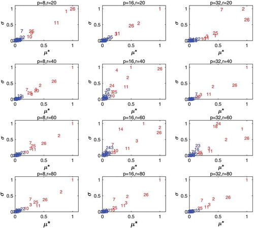
As mentioned in Section 3.3, the Morris method was applied with a different number of replications r (r = 20, 40, 60 and 80) and different levels (p = 8, 16 and 32). The main aim of this analysis is to successfully identify the sensitive model parameters by selecting the appropriate size of sample. Sensitivity measures, i.e. µ* and σ, were scaled to values between 0 and 1. A comparison of the absolute mean (µ*) and the standard deviation (σ) of the distribution function of each parameter for the three objective functions, NSE, RMSE and REVF, was carried out to evaluate the simulations.

Figures 5–7 show the results of different combinations of levels and replications for the objective functions NSE, RMSE and REVF, respectively. The sensitive (red numbers) and insensitive (blue numbers) labels were decided based on the threshold value of µ* = 0.15. Consistent results were not obtained, as is evident from Figures 5–7. The results in Row 1 (r = 20) are not identical to those with higher r (40, 60, 80). As the number of replications is increased, more model parameters are found to be significant. This clearly indicates the need to identify the correct number of replications for screening the SHETRAN model parameters. It may also be noticed that the same number of replications with different grid levels does not assure stable sensitivity results. In agreement with Yang (2011), we note that as the grid level (p) increases, the sensitivity ranks between model parameters are more distinguishable. The results of NSE and RMSE are similar in terms of their µ* value.

Figure 5. Sensitivity analysis results of Morris screening using different r and p for objective function NSE. Numbers in red are supposed to be sensitive parameters. The closer the parameter is to the upper right, the more sensitive it is.

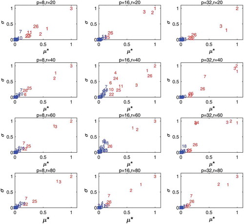
Figure 7. Sensitivity analysis results of Morris screening using different r and p for objective function REVF. Numbers in red are supposed to be sensitive parameters. The closer the parameter is to the upper right, the more sensitive it is.

Table 2 shows the sensitivity measures (µ* and σ) at grid level 32 for different numbers of replications (r) using NSE as the objective function. The values of sensitivity measures of model parameters display a closer similarity upon increasing the number of runs, due to higher replication times, r.

Table 2. Sensitivity measures (μ*: absolute mean; σ: standard deviation) of SHETRAN model parameters for objective function NSE evaluated at different r values (20, 40, 60 and 80) and grid level p = 32 using the Morris method.

Parameter no.	Parameter	μ*	σ	Parameter	μ*	σ
	r = 20			r = 40
1	Str1	0.810	0.307	Str1	1.000	0.825
2	Str2	1.000	1.000	Str2	0.990	1.000
3	Str3	0.711	0.436	Str3	0.956	0.923
7	kzm	0.023	0.037	kzm	0.427	0.661
9	THSATt	0.008	0.003	THSATt	0.010	0.006
11	THSATb	0.063	0.021	THSATb	0.164	0.094
22	kxm	0.195	0.045	kxm	0.167	0.049
24	dt	0.013	0.017	dt	0.008	0.010
25	dm	0.166	0.071	dm	0.183	0.121
26	db	0.231	0.159	db	0.386	0.272
	r = 60			r = 80
1	Str1	1.000	0.945	Str3	1	1
2	Str2	0.888	1.000	Str1	0.835	0.734
3	Str3	0.823	0.964	Str2	0.672	0.749
7	kzm	0.002	0.008	kzm	0.185	0.381
9	THSATt	0.267	0.930	THSATt	0.23	0.004
11	THSATb	0.090	0.069	THSATb	0.079	0.066
22	kxm	0.142	0.050	kxm	0.135	0.042
24	dt	0.280	0.955	dt	0.22	0.82
25	dm	0.157	0.079	dm	0.13	0.09
26	db	0.255	0.250	db	0.195	0.204

The Morris sensitivity indices did not differ much between sample sizes generated by 60 or 80 replications. Based on the results of this study, we recommend that, for a stable screening result, the number of replications should be 60 with a grid level of 32. The overall model runs were therefore 1620 simulations (r(k + 1), with k = 26, r = 60). The computational cost of one simulation was around 10 min using a PC with 3.2 GHz Intel® Pentium® processor.

A higher value of sensitivity measure µ* indicates that the parameter is highly relevant. Parameters with a µ* value of zero may be considered insignificant. A high value of σ indicates an interaction with other parameters or a nonlinear effect on the output (Saltelli et al. 2004). The parameters were ranked according to the value of the absolute mean (µ*) only, and the ranking of SHETRAN parameters for streamflow generation by Morris analysis is presented in Table 3. Considering NSE and RMSE as objective functions, the Strickler overland coefficient for the land-use classes agriculture, grass and forest is the most significant parameter, followed by the soil parameters depth of top, bottom and middle soil layers, denoted by dt, db and dm, respectively. The soil moisture of top and bottom soil layers (THSATt and THSATb) and the horizontal saturated hydraulic conductivity of the middle layer (kxm) are also significant. However, a slight difference in parameter rankings is observed based on objective function, e.g. Str is most sensitive for NSE and RMSE whereas db is most important for REVF. It can be further noted that, instead of kxm, van Genuchten α for the topsoil layer (ALFt) was significant when REVF was taken as the objective function. The parameters Str (for all land-use types), THSATt and dt (topsoil depth) also exhibit high σ values, indicating interaction of these parameters with others. The ranking of parameters for the dry season indicates the need to give due significance to subsurface parameter van Genuchten n (for the middle soil layer), the horizontal conductivities of all soil layers, and for the wet season, the vertical saturated conductivity of the middle soil layer.

Table 3. Morris screening ranking of SHETRAN model parameters to generate streamflow. NSE: Nash-Sutcliffe efficiency criterion; REVF: relative error of volumetric fit; RMSE: root mean square error. See Table 1 for parameter descriptions.

Rank	Parameter
	NSE	REVF	RMSE	NSEdry	NSEwet
1	Str1	db	Str1	Str1	Str3
2	Str2	Str1	Str2	Str3	Str1
3	Str3	Str2	Str3	Str2	Str2
4	dt	dt	dt	dm	db
5	THSATt	ALFt	THSATt	kxm	kzm
6	db	THSATb	db	dt	dm
7	dm	Str3	dm	kxt	kxm
8	kxm	THSATm	kxm	nm	THSATb
9	THSATb	dm	THSATb	kxb	THSATm

The parameter sensitivity results give an insight into the hydrological processes within the Netravathi River Basin. The high significance of land-use dependent surface parameters, i.e. Strickler overland coefficient, and subsurface parameters such as soil depth, saturated moisture content and horizontal saturated conductivity, controlling the baseflow, indicates that subsurface flow is a major component of streamflow for this river basin. This is in accordance with the study by Putty and Prasad (2000a), who reported that the hydrograph shape is governed by subsurface runoff in the Western Ghats region. The infiltration excess overland flow is negligibly small in this region and the variable source area theory (Dunne and Black 1970, Hewlett and Troendle 1975) describes the runoff processes in this region (Putty 1994, Putty and Prasad 1994). The landscape roughness, slope and drainage basin area are some of the factors affecting variable source areas (Lee and Delleur 1976). Hence, the highest rank for the Strickler overland coefficient (reciprocal of Manning’s roughness), which varies depending upon land-use type by sensitivity analysis for streamflow generation in the present study, is justified. Although the study area belongs to the tropics, low rainfall intensities with long durations occur in the region, influencing the soil depth and formation of natural pipes which contribute significantly to streamflow (Putty and Prasad 2000b). The effect of pipeflow on streamflow could be the possible reason for the insignificance of vertical saturated hydraulic conductivity and van Genuchten parameters, which describe retention of water in the soil mantle for this river basin.

It should be noted that the nature of hydrological processes and hence the model parameter sensitivities differ considerably depending on whether the region has an arid, semi-arid or tropical climate. The results presented in this study are generally applicable for a wet mountainous catchment in the tropics. The size of the analysed catchment is another factor determining the model parameter sensitivity. An application of the SHETRAN model to semi-arid basins in Iberia (Guerreiro et al. 2017) reported relatively small parameter sensitivity owing to the large catchment size, whereas in another semi-arid region (Cobres basin), the parameters van Genuchten α, AET/PET ratio, Strickler overland flow resistance coefficient, topsoil depth, van Genuchten n, and saturated and residual water content were sensitive, while saturated hydraulic conductivity was identified as insensitive (Zhang et al. 2013b). In a tropical West African basin, the AET/PET ratio had a strong influence on total runoff and the roughness parameter affected maximum runoff (Op de Hipt et al. 2017).

The Morris screening method fails to distinguish the nonlinearity of a factor from interaction with other factors and cannot provide accurate quantitative estimates of the contribution of a particular factor to the output variability (Yang 2011). However, for computationally expensive models having a multitude of parameters, the Morris method helps to identify the parameters having negligible effect on output variability and thereby acts as an efficient computational technique. The parameters that are found to be insensitive can be fixed in the calibration procedure without changing the prediction characteristics of the model.

4.2 Local sensitivity analysis

The effects of variation of Str and d, kx, kz, and θ_sat − θ_res on the peak total discharge (Q_max) are shown in Figures 8 and 9, respectively. The sensitivity of cumulative total discharge (Q_total) and cumulative overland discharge (Q_o) with variation in values of Str, kx, kz and θ_sat − θ_res was also analysed. Higher values of Strickler coefficient, Str, means lower roughness of the surface causing water to flow at a faster rate. An increase in the value of Str1 for the land-use type agriculture, covering 36% of the study area, from 0.02 to 100 m^1/3 s⁻¹ resulted in peak total discharge and peak overland flow increasing by 41% and 40%, respectively, whereas cumulative total outflow and cumulative overland flow increased by only 2%. Similarly, with an increase of Str3 from 0.09 to 10 m^1/3 s⁻¹ for the forest land-use type, the peak total discharge and peak overland flow increased by 1.7% and 30%, respectively, and cumulative total outflow by only 0.6%.

Figure 8. Sensitivity of peak total discharge to Strickler overland coefficient, Str. On the y-axis, “cumecs” is m³ s^−1.

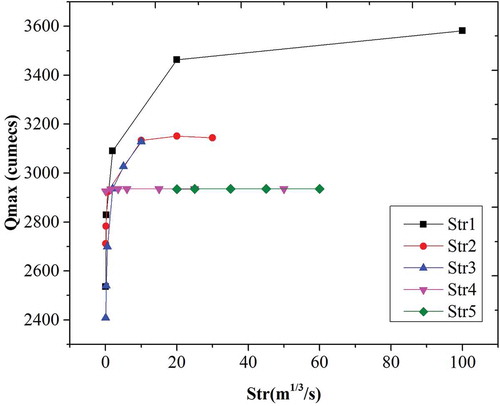
Figure 9. Sensitivity of peak total discharge to soil depth, horizontal saturated hydraulic conductivity (kx), vertical saturated hydraulic conductivity (kz) and θ_sat − θ_res in the top, middle and bottom soil layers.

Further, increasing the depth of different soil layers, i.e. the top, middle and bottom layers, caused the peak total discharge and the cumulative total outflow to decrease. The peak total outflow reduced by 0.07% and cumulative total discharge by 2% on increasing the depth of the bottom layer from 2 m to 20 m. Soil depth had an insignificant effect on peak and cumulative overland flow.

The peak total discharge was observed to decrease by only 2% and the cumulative total discharge decreased by only 1% on increasing the bottom layer horizontal conductivity from 0.0005 to 50 m/d. The simulations indicate that horizontal saturated conductivity values of the bottom soil layer in the range of 10–50 m/d lower the peak discharge of the Netravathi River Basin (Fig. 9). The top and middle soil layer horizontal conductivities had negligible effect on peak total discharge. The peak and cumulative overland flow were not affected by horizontal hydraulic conductivities.

However, no pronounced effect was produced on the peak total discharge upon varying the vertical saturated hydraulic conductivity of the three soil layers (Fig. 9). The effects on peak and cumulative overland flow were negligible due to variation in vertical saturated hydraulic conductivity.

The amount of water that soil can absorb is given by the available water content (AWC = θ_sat − θ_res) in the soil. The discharge is expected to be lower due to higher AWC, since the soil has greater capability to absorb water. An increase of AWC from 0.11 to 0.29 in the bottom soil layer and from 0.26 to 0.32 in the topsoil layer caused cumulative total discharge to decrease by a mere 0.1%, with negligible effect on peak total outflow (Fig. 9). Considering the total overland flow, increasing the AWC of the top layer from 0.2 to 0.32 resulted in a decrease in total overland flow by 0.6% and a negligible effect on peak overland flow.

Figure 10 shows the contribution of each model parameter to the total discharge. It may be noted that the change in Strickler overland coefficient value for land-use type agriculture (Str1) resulted in the highest change in total discharge by 1.6%, followed by Str2 (for grassland) resulting in a 1% increase in total discharge, corresponding to changes in Str values of 100 and 30 m^1/3 s⁻¹, respectively. Amongst the soil parameters, soil depth and horizontal saturated hydraulic conductivity of the bottom layer had the most influence in changing the total discharge by 1% due to change in d by 3 m and kxb by 100 m/d. The individual contributions of all other soil parameters on streamflow were found to be negligible.

Figure 10. Change (%) in total discharge due to change in parameter values for (a) Strickler overland coefficient, Str, and (b) soil parameters. Δ represents the change in parameter values.

The results of this investigation of the main model parameters affecting streamflow in the Netravathi River Basin are in consensus with other studies reported in this basin, although the hydrological models applied in those studies were different. The SWAT model parameter sensitivity in this basin revealed the highest significance for the land-use based surface parameter SCS runoff curve number, along with the baseflow-controlling parameters, soil hydraulic conductivity and available water capacity in the soil layer (Babar and Ramesh 2015, Sinha and Eldho 2018). The most sensitive VIC model parameters for Netravathi Basin were bi, governing the division of precipitation into infiltration and direct runoff, and thickness of the second layer d₂, affecting the water available for transpiration and baseflow, respectively, and Dm, representing maximum baseflow velocity (Madusudhanan et al. 2015). The SWAT and VIC model applications to the Netravathi River Basin indicate that the baseflow-controlling parameters are equally significant to the surface parameters for streamflow simulation.

4.3 Calibration and validation of the SHETRAN model

The initial screening by the Morris method helped in identifying the significant SHETRAN model parameters and, further, the local sensitivity analysis carried out quantified the effect of each model parameter on streamflow. The Morris analysis results were found to be in agreement with the local sensitivity results. The parameters identified as most significant – Str, soil depth (bottom layer), saturated moisture content for the daily streamflow simulation and the parameter kx (all soil layers) – were consequently varied between their upper and lower values to generate a new parameter sample size of 50, and insignificant parameter values were fixed in order to obtain the optimal model parameter values for streamflow generation. The SHETRAN model was run using these 50 samples to arrive finally at the optimal model parameters for streamflow simulation. The parameter ranges along with their optimal values obtained are presented in Table 4.

Table 4. Calibration parameters of SHETRAN: plausible ranges and optimal values (in parentheses). kz: vertical saturated conductivity; θ_sat: saturated water content; θ_res: residual water content.

Soil type	Clay loam	Sandy clay loam	Unknown	Land-use type	Strickler overland coefficient (m^1/3 s^−1)
Soil depth, d (m)	0.05–0.3 (0.3)	0.3–2.0 (1.5)	2.0–5.0 (5.0)	Agriculture	0.02–100 (5)
kz (m/d)	0.005–10 (0.01)	0.01–20 (0.2)	0.5–10.0 (5)	Grassland	0.05–30 (4)
kx (m/d)	0.001–10 (5)	0.00001–50 (10)	0.0005–20 (50)	Forest	0.09–10 (7)
θsat	0.4–0.5 (0.5)	0.41–0.5 (0.5)	0.2–0.42 (0.2)	Wasteland	0.08–50 (10)
θres	0.08–0.2 (0.09)	0.08–0.18 (0.09)	0.09–0.13 (0.09)	Urban	20–60 (25)

In order to assess the improvement in efficiency of the model in calibration using the results from the sensitivity analysis, simulations with uncalibrated and calibrated model parameters were compared. The statistical indices listed in Table 5 show that the calibration performed after the two-stage sensitivity analysis significantly improved the accuracy of the model. The NSE value of 0.277 before calibration indicates poor model performance, and this improved to 0.869 on a daily scale considering both the calibration and validation periods from 1989 to 1997. The values of correlation coefficient (R), RMSE and REVF obtained after calibration, in contrast to those obtained before calibration, show the improved model performance (Table 5).

Table 5. Model performance before and after calibration for the whole period (1989–1997).

	Daily		Monthly
	Before calibration	After calibration	Before calibration	After calibration
NSE	0.277	0.869	0.699	0.968
RMSE (mm)	9.393	5.547	177.707	69.517
R	0.778	0.934	0.883	0.985
REVF (%)	0.099	0.053	0.085	0.049

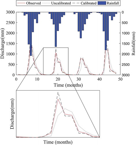
Figures 11 and 12 present the daily and monthly streamflow results, respectively, for the calibration period (1989–1993) and Figures 13 and 14 those for the validation period (1994–1997). The hydrographs clearly indicate that the peak flows are under-predicted and the baseflows over-predicted compared to the uncalibrated simulations on daily and monthly scales for both calibration and validation periods. However, the calibrated simulations could capture the peak flows and had a good match with the observed streamflow. The performance of the model for daily and monthly streamflow (Table 6) indicates the capability of the SHETRAN model to capture the hydrological processes within the Netravathi River Basin. The NSE value for the dry period is found to be satisfactory and indicates that the model could represent the flow released gradually by water stored within the soil matrix. NSE values of 0.89 and 0.83 were obtained for daily simulation for calibration and validation. The REVF values are close to zero and indicate that the observed runoff volume is simulated well by the SHETRAN model for the study area.

Table 6. Model performance measures for calibration and validation periods.

	Daily		Monthly
	Calibration	Validation	Calibration	Validation
NSE	0.89	0.83	0.97	0.96
RMSE (mm)	4.91	6.52	64.69	79.28
REVF (%)	0.11	0.002	0.11	0.003
NSEdry	0.51	0.83	0.77	0.86
NSEwet	0.81	0.80	0.92	0.95
R (dry)	0.82	0.92	0.90	0.97
R (wet)	0.90	0.89	0.97	0.97

Figure 11. SHETRAN daily streamflow predictions with the calibrated and uncalibrated parameters compared to the observed flows – calibration period (1989–1993). Zoom windows show daily discharge for 1990.

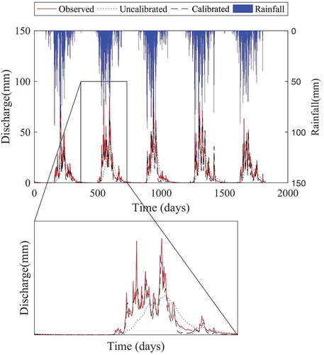
Figure 12. SHETRAN monthly streamflow predictions with the calibrated and uncalibrated parameters compared to the observed flows – calibration period (1989–1993). Zoom windows show monthly discharge for 1990.

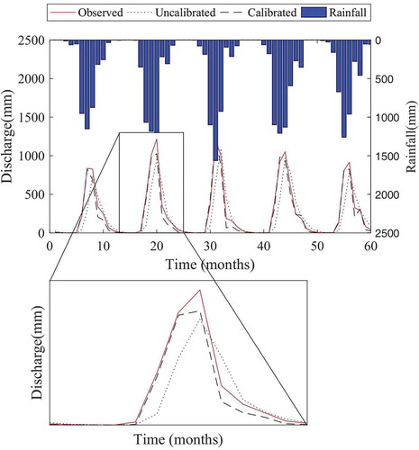
Figure 13. SHETRAN daily streamflow predictions with the calibrated and uncalibrated parameters compared to the observed flows – validation period (1994–1997). Zoom windows show monthly discharge for 1995.

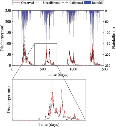
Figure 14. SHETRAN monthly streamflow predictions with the calibrated and uncalibrated parameters compared to the observed flows – validation period (1994–1997). Zoom windows show monthly discharge for 1995.

5 Conclusions

In this paper, a systematic approach for parameter sensitivity analysis and calibration of a physically-distributed, hydrological model for a river basin is presented. The Morris method was implemented to identify the most significant SHETRAN model parameters for streamflow generation in the Netravathi River Basin. Further, local sensitivity analysis performed in the study could quantify the influence of individual model parameters on the streamflow. Based on the information from sensitivity analysis, the SHETRAN model was calibrated for streamflow in the Netravathi River Basin. The major observations resulting from the study are as follows:

The most relevant SHETRAN parameters identified by the Morris method include the land-use parameter, Strickler overland coefficient, controlling the surface flow, and baseflow-controlling parameters, namely soil depth, horizontal saturated hydraulic conductivity (middle soil layer) and soil moisture content. The parameter sensitivity rankings indicate that the baseflow contribution is equally important as surface flow for streamflow generation in the Netravathi River Basin. Twenty-six model parameters were assessed using 1620 model simulations for different Morris samples and 10 model parameters were identified as most significant for streamflow.

For a distributed model such as SHETRAN, the Morris global sensitivity analysis method is an effective screening technique to identify the insignificant parameters. The method could also demonstrate the interactions that exist between model parameters which significantly influence the values of other parameters. The parameters Str (of all land-use types), saturated moisture content of topsoil (THSATt) and topsoil depth were identified to have strong interactions with other parameters.

When applying the Morris method, it is essential to check the stability of ranking parameters by using different sample sizes. Our study identified a grid level of 32 and number of replications of 60 for convergence of parameter rankings. Although the parameter rankings did not show a notable difference between dry and wet periods, parameters such as van Genuchten n for the dry period and vertical saturated hydraulic conductivity for the wet period were found to be relevant.

The local sensitivity analysis revealed that the most sensitive parameter is the Strickler overland coefficient, which varies with land-use type. Soil depth of the bottom layer and its horizontal saturated conductivity significantly influence streamflow in the basin. Thus, the parameter ranking obtained by the Morris method agrees well with the results of the local sensitivity analysis method.

Model calibration of the most significant model parameters can be performed with few SHETRAN model runs. The sensitivity analysis procedure may aid in accelerating the calibration procedure with the identification of those parameters to be given due importance and those parameters that could be given a fixed value.

The different statistical indices (NSE, RMSE, R and REVF) used to evaluate simulated streamflow with respect to observed streamflow indicated the capability of the SHETRAN model to simulate the streamflow for the Netravathi River Basin in the Western Ghats region of India. The two-stage procedure implemented in this study may be used to simplify the manual calibration of the SHETRAN model and could give statistically significant improvement to the model performance for simulating the streamflow.

The model parameter sensitivity results presented in this study pertain to a wet, mountainous, tropical Western Ghats river basin and are likely to differ depending upon the hydrological processes of the catchment analysed.

The Morris and local sensitivity analysis methods are model independent. Hence, the two-stage procedure implemented in this study could be applied to other complex hydrological models having a multitude of input parameters and thus reduce the effort required for model calibration.

Acknowledgments

The authors acknowledge the Directorate of Economics and Statistics, Karnataka, and the India Meteorological Department for sharing rainfall and meteorological data for this study; the Central Water Commission for providing streamflow data; and Dr Birkinshaw, School of Civil Engineering and Geosciences; Newcastle University, UK, for great assistance in clearing all the SHETRAN-related queries. The first author acknowledges Dr Suraj Harshan, former Research Assistant, Department of Geography, National University of Singapore, for helpful discussions on sensitivity analysis. The national supercomputing facility PARAM Yuva at C-DAC, Pune, is acknowledged for providing the computational facilities. The authors acknowledge the editorial board and anonymous reviewers for their critical comments which improved the manuscript.

Disclosure statement

No potential conflict of interest was reported by the authors.

Supplementary material

Supplemental data for this article can be accessed here.

References

- Abebe, N., Ogden, F., and Pradhan, N., 2010. Sensitivity and uncertainty analysis of the conceptual HBV rainfall–runoff model: implications for parameter estimation. Journal of Hydrology, 389 (3–4), 301–310. doi:10.1016/j.jhydrol.2010.06.007
- Anderton, S., Latron, J., and Gallart, F., 2002. Sensitivity analysis and multi-response, multi-criteria evaluation of a physically based distributed model. Hydrological Processes, 16 (2), 333–353. doi:10.1002/hyp.336
- Azim, F., Sattar, A., Habib-ur-Rehman, and Kanwal, A., 2016. Impact of climate change on sediment yield for Naran watershed. International Journal of Sediment Research, 31 (3), 212–219. Elsevier. doi:10.1016/j.ijsrc.2015.08.002
- Babar, S. and Ramesh, H., 2015. Streamflow response to land use – land cover change over the Nethravathi river basin, India. Journal of Hydrologic Engineering, 20 (10), 05015002. doi:10.1061/(ASCE)HE.1943-5584.0001177
- Bahremand, A. and De Smedt, F., 2008. Distributed hydrological modeling and sensitivity analysis in Torysa watershed, Slovakia. Water Resources Management, 22 (3), 393–408. doi:10.1007/s11269-007-9168-x
- Bathurst, J., et al., 2006. Application of the SHETRAN basin-scale, landslide sediment yield model to the Llobregat basin, Spanish Pyrenees. Hydrological Processes, 20, 3119–3138. doi:10.1002/hyp.6151
- Bathurst, J., et al., 2004. Validation of catchment models for predicting land-use and climate change impacts. 3. Blind validation for internal and outlet responses. Journal of Hydrology, 287 (1–4), 74–94. doi:10.1016/j.jhydrol.2003.09.021
- Benedetti, L., Baets, B. De, Nopens, I., and Vanrolleghem, P.A., 2010. Multi-criteria analysis of wastewater treatment plant design and control scenarios under uncertainty. Environmental Modelling and Software, 25 (5), 616–621. Elsevier Ltd. doi:10.1016/j.envsoft.2009.06.003
- Benke, K.K., Lowell, K.E., and Hamilton, A.J., 2008. Parameter uncertainty, sensitivity analysis and prediction error in a water-balance hydrological model. Mathematical and Computer Modelling, 47, 1134–1149. doi:10.1016/j.mcm.2007.05.017
- Beven, K. and Binley, A., 1992. The future of distributed models: model calibration and uncertainty prediction. Hydrological Processes, 6 (3), 279–298. doi:10.1002/(ISSN)1099-1085
- Beven, K.J., Warren, R.O.S.S., and Zaoui, J., 1980. SHE: towards a methodology for physically-based distributed forecasting in hydrology. In: Hydrological forecasting (Proceedings of the Oxford Symposium, April 1980). Wallingford, UK: International Association of Hydrological Sciences, IAHS Publ. no. 129, 133–138. Available from: http://hydrologie.org/redbooks/a129/iahs_129_0133.pdf [Accessed 26 March 2019].
- Birkinshaw, S.J., 2010. Technical note : automatic river network generation for a physically-based river catchment model. Hydrology and Earth System Sciences, (14), 1767–1771. doi:10.5194/hess-14-1767-2010
- Birkinshaw, S.J., et al., 2011. The effect of forest cover on peak flow and sediment discharge-an integrated field and modelling study in central-southern Chile. Hydrological Processes, 25 (8), 1284–1297. doi:10.1002/hyp.7900
- Birkinshaw, S.J., et al., 2016. Climate change impacts on Yangtze river discharge at the three gorges dam. Hydrology and Earth System Sciences, 21 (4), 1–33. doi:10.5194/hess-2016-231
- Blaney, H.F. and Criddle, W.D., 1950. Determining Water Requirements in Irrigated Areas from Climatological and Irrigation Data USDA-SCS-TP-96 Report 50. Washington, DC.
- Bonell, M., et al., 2010. The impact of forest use and reforestation on soil hydraulic conductivity in the Western Ghats of India : implications for surface and sub-surface hydrology. Journal of Hydrology, 391 (1–2), 47–62. Elsevier B.V. doi:10.1016/j.jhydrol.2010.07.004
- Bovolo, C.I., et al., 2009. A distributed framework for multi-risk assessment of natural hazards used to model the effects of forest fire on hydrology and sediment yield. Computers and Geosciences, 35 (5), 924–945. doi:10.1016/j.cageo.2007.10.010
- Brazier, R.E., et al., 2000. Equifinality and uncertainty in physically based soil erosion models: application of the GLUE methodology to WEPP - the water erosion prediction project - for sites in the UK and USA. Earth Surface Processes and Landforms, 25, 825–845. doi:10.1002/(ISSN)1096-9837
- Campolongo, F., Cariboni, J., and Saltelli, A., 2007. An effective screening design for sensitivity analysis of large models. Environmental Modelling and Software, 22 (10), 1509–1518. doi:10.1016/j.envsoft.2006.10.004
- Carpenter, T.M., Georgakakos, K.P., and Sperfslagea, J.A., 2001. On the parametric and NEXRAD-radar sensitivities of a distributed hydrologic model suitable for operational use. Journal of Hydrology, 253 (253), 169–193. doi:10.1016/S0022-1694(01)00476-0
- Central Water Commission, 2006. Integrated hydrological data book. India: New Delhi.
- Chow, V.T., 1959. Open-channel hydraulics. New York: McGraw-Hill.
- Cibin, R., Sudheer, K.P., and Chaubey, I., 2010. Sensitivity and identifiability of stream flow generation parameters of the SWAT model sensitivity and identifiability of stream flow generation. Hydrological Processes, 24 (9), 1133–1148. doi:10.1002/hyp.7568
- Demaria, E.M., Nijssen, B., and Wagener, T., 2007. Monte Carlo sensitivity analysis of land surface parameters using the variable infiltration capacity model. Journal of Geophysical Research, 112, 1–15. doi:10.1029/2006JD007534
- Đukić, V. and Radić, Z., 2016. Sensitivity analysis of a physically based distributed model. Water Resources Management, 30. doi:10.1007/s11269-016-1243-8
- Dunne, T. and Black, R.D., 1970. Partial area contributions to storm runoff in a small New England watershed. Water Resources Research, 6 (5), 1296–1311. doi:10.1029/WR006i005p01296
- Elliott, A.H., et al., 2012. Sediment modelling with fine temporal and spatial resolution for a hilly catchment. Hydrological Processes, 26 (24), 3645–3660. doi:10.1002/hyp.8445
- Ewen, J. and Parkin, G., 1996. Validation of catchment models for predicting land-use and climate change impacts. 1. Method. Journal of Hydrology, 175 (1–4), 583–594. doi:10.1016/S0022-1694(96)80026-6
- Ewen, J., Parkin, G., and Connell, P.E., 2000. SHETRAN: distributed river basin flow modeling system. Journal of Hydrologic Engineering, 5 (3), 250–258. doi:10.1061/(ASCE)1084-0699(2000)5:3(250)
- FAO/IIASA/ISRIC/ISSCAS/JRC, 2012. Harmonized world soil database (version 1.2).FAO. Available from http://www.fao.org/soils-portal/soil-survey/soil-maps-and-databases/harmonized-world-soil-database-v12/en/
- Francos, A., et al., 2003. Sensitivity analysis of distributed environmental simulation models : understanding the model behaviour in hydrological studies at the catchment scale. Reliability Engineering and System Safety, 79, 205–218. doi:10.1016/S0951-8320(02)00231-4
- Gan, Y., et al., 2014. Environmental modelling and software A comprehensive evaluation of various sensitivity analysis methods : A case study with a hydrological model. Environmental Modelling and Software, 51, 269–285. doi:10.1016/j.envsoft.2013.09.031
- Guerreiro, S.B., et al., 2017. Dry getting drier − the future of transnational river basins in Iberia. Journal of Hydrology, Regional Studies, 12, 238–252. Elsevier. doi:10.1016/j.ejrh.2017.05.009
- Gupta, H.V., Sorooshian, S., and Yapo, P.O., 1998. Toward improved calibration of hydrologic models : multiple and noncommensurable measures of information. Water Resources Research, 34 (4), 751–763. doi:10.1029/97WR03495
- Herman, J.D., et al., 2013. Method of Morris effectively reduces the computational demands of global sensitivity analysis for distributed watershed models. Hydrology and Earth System Sciences, 17 (7), 2893–2903. doi:10.5194/hess-17-2893-2013
- Hewlett, J.D. and Troendle, C., 1975. Non point and diffused water sources: a variable source area problem. In: Symposium on watershed management. Logan, UT: Utah State University, ASCE, 21–46.
- Holvoet, K., et al., 2005. Sensitivity analysis for hydrology and pesticide supply towards the river in SWAT. Physics and Chemistry of the Earth, Parts A/B/C, 30 (8–10), 518–526. doi:10.1016/j.pce.2005.07.006
- Hornberger, G. and Spear, R., 1981. An approach to the preliminary analysis of environmental systems. Journal of Environmental Management, 12 (1), 7–18.
- Kelleher, C., Wagener, T., and McGlynn, B., 2015. Model based analysis of the influence of catchment properties on hydrologic partitioning across five mountain headwater subcatchments. Water Resources Research, 51, 4109–4136. doi:10.1002/2014WR016147
- Lee, M.T. and Delleur, J., 1976. A variable source area model of the rainfall‐runoff process based on the watershed stream network. Water Resources Research, 12 (5), 1029–1036.
- Lenhart, T., et al., 2002. Comparison of two different approaches of sensitivity analysis. Physics and Chemistry of the Earth, Parts A/B/C, 27, 645–654.
- Madusudhanan, C., Eldho, T.I., and Pai, D., 2015 .Hydrological impacts of climate change in a humid tropical River basin. In: Proc. 36th IAHR World Congr. Hague, Netherlands.
- Matthews, C.J., et al., 2007. Analysing the sensitivity behaviour of two hydrology models. Environmental Modelling and Assessment, 12, 27–41. doi:10.1007/s10666-006-9049-3
- Moriasi, D.N., et al., 2007. Model evaluation guidelines for systematic quantification of accuracy in watershed simulations. Transactions of the American Society of Agricultural and Biological Engineers, 50 (3), 885–900. doi:10.13031/2013.23153
- Morris, M.D., 1991. Factorial sampling plans for preliminary computational experiments. Technometrics, 33 (2), 161–174. doi:10.1080/00401706.1991.10484804
- Mourato, S., Moreira, M., and Corte-Real, J., 2015. Water resources impact assessment under climate change scenarios in Mediterranean watersheds. Water Resources Management, 29 (7), 2377–2391. doi:10.1007/s11269-015-0947-5
- Muleta, M.K., 2012. Improving model performance using season-based evaluation. Journal of Hydrologic Engineering, 17, 191–200.
- Muleta, M.K. and Nicklow, J.W., 2005. Sensitivity and uncertainty analysis coupled with automatic calibration for a distributed watershed model. Journal of Hydrology, 306, 127–145. doi:10.1016/j.jhydrol.2004.09.005
- Nash, J.E. and Sutcliffe, J.V., 1970. River flow forecasting through conceptual models part I—A discussion of principles. Journal of Hydrology, 10 (3), 282–290.
- Norton, J., 2015. An introduction to sensitivity assessment of simulation models. Environmental Modelling and Software, 69, 166–174. doi:10.1016/j.envsoft.2015.03.020
- Nossent, J., Elsen, P., and Bauwens, W., 2011. Sobol’ sensitivity analysis of a complex environmental model. Environmental Modelling and Software, 26 (12), 1515–1525. doi:10.1016/j.envsoft.2011.08.010
- Op de Hipt, F., et al., 2017. Applying SHETRAN in a TropicalWest African catchment (Dano, Burkina Faso)—calibration, validation, uncertainty assessment. Water, 9 (2), 101. doi:10.3390/w9020101
- Osuch, M., Romanowicz, R.J., and Booij, M.J., 2015. The influence of parametric uncertainty on the relationships between HBV model parameters and climatic characteristics HBV model parameters and climatic characteristics. Hydrological Sciences Journal, 60 (7–8), 1299–1316. doi:10.1080/02626667.2014.967694
- Pan, S., et al., 2017. A two-step sensitivity analysis for hydrological signatures in Jinhua River Basin, East China. Hydrological Sciences Journal, 62 (15), 2511–2530. doi:10.1080/02626667.2017.1388917
- Pujol, G., Iooss, B., and Janon, A., 2015. Sensitivity analysis package, R package version 1.11.1. Available from: http://cran.r-project.org/web/packages/sensitivity/index.html [Accessed 12 June 2015].
- Putty, M.R.Y., 1994. The mechanisms of streamflow generation in the Sahyadri Ranges (Western Ghats) of South India. Thesis (PhD). Indian Institute of Science, Bangalore.
- Putty, M.R.Y. and Prasad, R., 1994. Streamflow generation in the Western Ghats. In: Procedings Sixth National Sympsium Hydrology. Shillong, India, 189–194.
- Putty, M.R.Y. and Prasad, R., 2000a. Understanding runoff processes using a watershed model — a case study in the Western Ghats in South India. Journal of Hydrology, 228 (3–4), 215–227.
- Putty, M.R.Y. and Prasad, R., 2000b. Runoff processes in headwater catchments — an experimental study in Western Ghats, South India. Journal of Hydrology, 235 (1–2), 63–71.
- Rakovec, O., et al., 2014. Distributed evaluation of local sensitivity analysis (DELSA), with application to hydrologic models. Water Resources Research, 50 (1), 409–426. doi:10.1002/2013WR014063
- Ratto, M., et al., 2007. Uncertainty, sensitivity analysis and the role of data based mechanistic modeling in hydrology. Hydrology and Earth System Sciences, 11, 1249–1266.
- Refsgaard, J.C., 1997. Parameterisation, calibration and validation of distributed hydrological models. Journal of Hydrology, 198, 69–97.
- Ruano, M.V., et al., 2011. Application of the Morris method for screening the in fl uential parameters of fuzzy controllers applied to wastewater treatment plants. Water Sience Technology, 63 (10), 2199–2206. doi:10.2166/wst.2011.442
- Saltelli, A., Tarantola, S., and Campolongo, F., 2000. Sensitivity analysis as an ingredient of modeling. Statistical Science, 15 (4), 377–395.
- Saltelli, A., et al., 2004. Sensitivity analysis in practice: a guide to assessing scientific models. Chichester, England: Wiley.
- Sarrazin, F., Pianosi, F., and Wagener, T., 2016. Global sensitivity analysis of environmental models: convergence and validation. Environmental Modelling and Software, 79, 135–152. doi:10.1016/j.envsoft.2016.02.005
- Shetkar, R. and Mahesha, A., 2011. Tropical, seasonal river basin development : hydrogeological analysis. Journal of Hydrologic Engineering, 16 (3), 280–291. doi:10.1061/(ASCE)HE.1943-5584.0000328
- Sieber, A. and Uhlenbrook, S., 2005. Sensitivity analyses of a distributed catchment model to verify the model structure. Journal of Hydrology, 310 (1–4), 216–235. doi:10.1016/j.jhydrol.2005.01.004
- Sinha, R.K. and Eldho, T.I., 2018. Effects of historical and projected land use/cover change on runoff and sediment yield in the Netravati river basin, Western Ghats, India. Environmental Earth Sciences, 77 (3), 111. Springer Berlin Heidelberg. doi:10.1007/s12665-018-7317-6
- Sobol‘, M., 1993. Sensitivity estimates for nonlinear mathematical models. Mathematical Modelling in Civil Engineering (MMCE), 1 (4), 407–414.
- Spruill, C.A., Workman, S.R., and Taraba, J.L., 2000. Simulation of daily and monthly stream discharge from small watersheds using the SWAT model. Transactions of the ASAE, 43 (6), 1431–1439.
- Sun, X.Y., et al., 2012. Three complementary methods for sensitivity analysis of a water quality model. Environmental Modelling and Software, 37, 19–29. doi:10.1016/j.envsoft.2012.04.010
- Tang, Y., et al., 2007. Advancing the identification and evaluation of distributed rainfall-runoff models using global sensitivity analysis. Water Resources Research, 43, 1–14. doi:10.1029/2006WR005813
- Tarantola, S., et al., 2002. Can global sensitivity analysis steer the implementation of models for environmental assessments and decision-making? Stochastic Environmental Research and Risk Assessment, 16 (1), 63–76.
- Tong, C., 2010. Self-validated variance-based methods for sensitivity analysis of model outputs. Reliability Engineering and System Safety, 95 (3), 301–309. Elsevier. doi:10.1016/j.ress.2009.10.003
- van Griensven, A., et al., 2006. A global sensitivity analysis tool for the parameters of multi-variable catchment models. Journal of Hydrology, 324 (324), 10–23. doi:10.1016/j.jhydrol.2005.09.008
- Van Werkhoven, K., et al., 2008. Characterization of watershed model behavior across a hydroclimatic gradient. Water Resources Research, 44, 1–16. doi:10.1029/2007WR006271
- Wagener, T., 2003. Evaluation of catchment models. Hydrological Processes, 17, 3375–3378. doi:10.1002/hyp.5158
- Wagener, T. and Kollat, J., 2007. Visual and numerical evaluation of hydrologic and environmental models using the Monte Carlo analysis toolbox (MCAT) numerical and visual evaluation of hydrological and environmental models using the Monte Carlo analysis toolbox. Environmental Modelling and Software, 22, 1021–1033. doi:10.1016/j.envsoft.2006.06.017
- Yang, J., 2011. Convergence and uncertainty analyses in Monte-Carlo based sensitivity analysis. Environmental Modelling and Software, 26 (4), 444–457. doi:10.1016/j.envsoft.2010.10.007
- Yang, J., et al., 2012. Multi-objective sensitivity analysis of a fully distributed hydrologic model WetSpa. Water Resources Management, 26, 109–128. doi:10.1007/s11269-011-9908-9
- Ye, Y., et al., 2014. Parameter identification and calibration of the Xin’anjiang model using the surrogate modeling approach. Frontiers of Earth Science, 8 (2), 264–281. doi:10.1007/s11707-014-0424-0
- Zelelew, M. and Alfredsen, K., 2013. Sensitivity-guided evaluation of the HBV hydrological model parameterization. Journal of Hydroinformatics, 15 (3). doi:10.2166/hydro.2012.011
- Zhang, C., Chu, J., and Fu, G., 2013a. Sobol’s sensitivity analysis for a distributed hydrological model of Yichun River Basin, China. Journal of Hydrology, 480, 58–68. Elsevier B.V. doi:10.1016/j.jhydrol.2012.12.005
- Zhang, R., et al., 2013b. Automatic calibration of the SHETRAN hydrological modelling system using MSCE. Water Resources Management, 27, 4053–4068. doi:10.1007/s11269-013-0395-z