Assessment of geomorphological bank evolution of the alluvial threshold rivers based on entropy concept parameters

ABSTRACT

The complex stream bank profiles in alluvial channels and rivers that are formed after reaching equilibrium has been a popular topic of research for many geomorphologists and river engineers. The entropy theory has recently been successfully applied to this problem. However, the existing methods restrict the further application of the entropy parameter to determine the cross-section slope of the river banks. To solve this limitation, we introduce a novel approach in the extraction of the equation based on the calculation of the entropy parameter (λ) and the transverse slope of the bank profile at threshold channel conditions. The effects of different hydraulic and geometric parameters are evaluated on a variation of the entropy parameter. Sensitivity analysis on the parameters affecting the entropy parameter shows that the most effective parameter on the λ-slope multiplier is the maximum slope of the bank profile and the dimensionless lateral distance of the river banks.

KEYWORDS:

• stable channel
• entropy
• transverse slope
• bank profile
• river geomorphology
• uncertainty

Editor R. WoodsAssociate editor A. Petroselli

1 Introduction

Channel stability is referred to as an equilibrium state in which the shape and dimensions of the channel cross-section show no further change with the movement of flow in the channel (Nanson and Huang 2018). The process of reaching the equilibrium in straight channels is complex. After this transient stage, the stream will reach the equilibrium stage, where no sediments are deposited on the banks and bank particles are on the threshold of motion (stable cross-section state), or so-called static equilibrium (Yu and Knight 1998). In this case, there is no change in the dimensions and shape of the channel cross-section. Extensive studies have been performed on the morphology of alluvial streams and the geometric dimensions of the channel in dynamic equilibrium or regime (Singh 2003, Millar 2005, Afzalimehr et al. 2010, Huang et al. 2014, Kaless et al. 2014, Julien 2015, Bonakdari and Gholami 2016, Eaton and Millar 2017, Gholami et al. 2017a, Métivier et al. 2017, Shaghaghi et al. 2017, 2018a, 2018b, Joshi et al. 2018). However, a key knowledge gap is the cross-sectional shape and the slope of the bank profiles in the threshold state of the straight channel. The paradox problem of the stable channels is explained by the analytical model of the redistribution of shear stress on the channel banks due to the longitudinal transition of lateral momentum caused by turbulence impact on flows, given by Parker (1978). Considering the momentum transition term, a cosine profile for the threshold channel banks was suggested by Parker (1978). Pizzuto (1990) performed a numerical simulation of the water surface widening in the threshold channel. He stated that the slope on the banks caused by erosion would reach the equilibrium channel if it becomes larger than the angle of sediment repose (φ). Therefore, the designed stable channel based on their model is an exponential function that is almost similar to the classic cosine model. Diplas (1990) conducted extensive laboratory studies and validated the diffusion equations provided by Parker (1978). The proposed equation was similar to the equation of Ikeda (1981), who estimated the bank shapes of the channel as an exponential function. However, the presence of the coefficient k as the displacement thickness was limited to the application of the proposed equation by Ikeda (1981), due to the complexity of determining it. Later, Diplas and Vigilar (1992) proposed a polynomial shape for the banks of channels by a numerical solution of the momentum equilibrium for the fluid and the balance of forces for sediment particles at the threshold. They reported the stability of the banks in polynomial form and the instability of other previously presented shapes. Vigilar and Diplas (1998) provided equations and graphical solutions for designing the stable channel using a numerical model (Vigilar and Diplas 1997). Dey (2001) proposed a polynomial shape for stable channel banks using the momentum equation based on a power law. Khodashenas (2016) measured the bank profile shape of stable channels experimentally and evaluated the ability of different traditional models based on experimental datasets. They stated that the polynomial shape of stable bank profiles proposed by Vigilar and Diplas (1998) has more conformity with experimental data. Gholami et al. (2018a, 2018d, 2018c) examined the application of artificial intelligence (AI) methods, such as gene expression programming (GEP) and adaptive neuro-fuzzy inference system (ANFIS) in predicting bank profile shapes of stable channels. Their results demonstrated an acceptable agreement of these AI methods with the corresponding observed values.

Figure 1. Definition of the notation in the cross-section of a threshold channel.

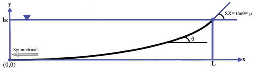
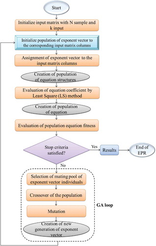
Figure 2. Flowchart of the proposed EPR model.

Almost three decades ago, the entropy theory and probability concept were applied to hydraulic open channels by Chiu (1987), who derived Shannon entropy-based equations for the velocity distribution and sediment transport in open channels. Following the study by Chiu (1987), other researchers carried out many studies on the application of the entropy concept for formulating velocity and shear stress distribution (e.g. Sterling and Knight 2002, Chiu et al. 2005, Moramarco and Singh 2010, Luo and Singh 2011, Bonakdari 2012, Cui and Singh 2013, Kumbhakar et al. 2017, Khozani and Bonakdari 2018, Kundu 2018) to ensure successful application of the entropy-based velocity equation in practical cases. A decade after the application of entropy in the estimation of the velocity distribution, Cao and Knight (1997) were the first to use the concept of entropy to examine the slope of the bank of threshold alluvial channels. They provided a parabolic equation from the Shannon entropy concept for stable channel banks that was in good agreement with observed results. The obtained equation for transverse slope followed the same format as the velocity distribution and contained the Lagrange multiplier (λ). The Lagrange multiplier is created during maximizing the entropy equation subject to its constraints in order to obtain the transverse slope distribution of stable channels banks. This multiplier is referred to as the “entropy parameter” in this paper.

The entropy parameter is one of the key parameters in the entropy approach. The profile shape of stable channels is highly dependent on the values of the entropy parameter (Cao and Knight 1997), which has a physical meaning that should be examined further. Therefore, the entropy parameter should be linked to some suitable hydraulic parameters, or be connected with the boundary conditions of the channel. The entropy parameter (λ) was numerically justified by the study of Cao and Knight (1997), who, with consideration of an ideal state for the channel cross-section, based on Chow (1959), eliminated the λ multiplier in the entropy equation of the transverse slope (S_t) of the channel. They referred to the hydraulic concept of this parameter and its significant effects on the estimation of S_t. In their studies, they explicitly emphasized the detailed calculations of the entropy parameter (λ) in entropy theory and the necessity of further studies on the formulation and physical basis of this parameter. In the study by Cao and Knight (1997), no equation is presented for calculating the λ multiplier, so it is considered necessary to provide a relationship based on this parameter for calculating S_t using different observational datasets. Sterling and Knight (2002) emphasized this subject in presenting a model based on the Shannon entropy theory in shear stress distribution. Their results indicated the model’s weakness in predicting shear stress due to its strong dependence on the multiplier λ; although an empirical equation is presented for calculating the entropy parameter, there is no physical interpretation of it. Hence, they pointed to the importance of this parameter and the need for further studies on it.

Considering the previous studies on entropy theory and the emphasis on the necessity for further studies on the evaluation of the λ parameter and the factors affecting it, our study is based on the concept of Shannon entropy theory. Therefore, in this study, an equation for calculating this multiplier is presented that can be solved numerically in MATLAB and the obtained λ values are evaluated. In addition, to our knowledge, no study has been done to evaluate various hydraulic variables using the entropy theory on the physical concept of the entropy parameter (λ) and effective factors on it, especially in the case of the transverse slope of river bank profiles. Changes in the parameters in the terms of several sets of observational data are examined in detail and evaluated with different hydraulic and geometric conditions. In addition, an equation for calculating this multiplier based on entropy theory is presented. The effects of geometric factors (maximum bank slope, μ, and coordinates of the points located on the stable boundary) and hydraulic parameters (flow rate, Q; median sediment size, d₅₀; and maximum flow depth at the channel centre line, h_c) on the changes in the entropy parameter are evaluated using a numerical model based on soft computing. Finally, the relationship based on these variables is presented and evaluated for the calculation of the entropy parameter.

2 Materials and method

2.1 Modified Shannon entropy model for transverse slope of threshold channels

The event probability of a variable can be calculated from the entropy concept, provided that the distribution of that variable is in accordance with the rules governing entropy (Atieh et al. 2015, 2017, Bonakdari et al. 2015, Pechlivanidis et al. 2016, Liu et al. 2017, Silva et al. 2017). One of the most popular entropies, the Shannon entropy, was first introduced by Shannon (1948) as presented below:

(1) $H=-\int \mathrm{p}(x)ln\mathrm{p}(x)\mathrm{d}x$(1)

where p(x) is the probability density function of the desired variable (x), p(x)dx is the event probability of the desired variable at the interval x to x + dx and H is the entropy value of that variable. Now, by using the principle of maximum entropy (Jowitt 1991), the probability distribution of that variable will be as uniform as possible, while satisfying the constraint. In Equation (1), the studied variable is the transverse slope (S_t) of the threshold channels. Also, the maximization rule for the entropy value can be used to find the probability density function of the channel transverse slope.

The governing constraint condition in this study is investigated for the asymmetric cross-section of alluvial channels with a boundary level equal to 0 in the central line of the channel and a half-width of L (the channel width, B, is equal to 2L). The minimum value of the transverse slope of the bank profile in the central line of the channel (x = 0), with a boundary level equal to zero (y = 0), is zero. The maximum transverse slope (SX) in the water margin at the transverse distance L from the central line of the channel (x = L), with the boundary level equal to the maximum depth at the channel centre (y = h_c), is equal to μ (static coefficient of Coulomb friction) (Ikeda et al. 1988, Pizzuto 1990) (Fig. 1). With the constraint condition defined for the bank profiles of stable channels, it can be said that the transverse slope of the bank profile is uniformly distributed between its maximum and minimum values. In fact, for each point on the bank profile with a transverse distance of less than L, the S_t value is less than SX. In this case, the cumulative distribution function for the transverse slope of the bank profile of a stable channel can be considered as:

(2) $F(S_{\mathrm{t}})=\frac{x}{L}$(2)

The Shannon entropy equation for the threshold channel transverse slope is as follows (Cao and Knight 1997):

(3) $H(S_{\mathrm{t}})=-\int \mathrm{p}(S_{\mathrm{t}})ln\mathrm{p}(S_{\mathrm{t}})\mathrm{d}{S}_{\mathrm{t}}$(3)

in which two entropy constraints are defined (Equations (4) and (5)), the first being the definition of the overall probability rule:

(4) ${\int }_0^{\mu }\mathrm{p}(S_{\mathrm{t}})\mathrm{d}{S}_{\mathrm{t}}=1$(4)

(5) ${\int }_0^{\mu }\mathrm{p}(S_{\mathrm{t}})\mathrm{d}{S}_{\mathrm{t}}={\bar{S}}_{\mathrm{t}}$(5)

In Equation (5), ${\bar{S}}_{\mathrm{t}}$ is the mean transverse slope for the cross-sectional profile, which is equal to the ratio of the depth at the centre of the channel (h_c) to the transverse distance in the water margin (L), and is shown as SN herein. In both constraints (4) and (5), the lower and upper limits of the integral (0 and μ) are, respectively, the minimum (at the channel centre, x = 0) and maximum transverse slope of the bank profile.

The probability density distribution function p(S_t) should be able to satisfy the two constraint conditions (Equations (4) and (5)). To maximize H(S_t) and to achieve the transverse slope distribution p(S_t) equation, the following differential equation is obtained using the Lagrange multiplier method (LMM), with the two Lagrange multipliers of λ and λ₁:

(6) $\frac{\mathrm{\partial }\left(-\mathrm{p}(S_{\mathrm{t}})ln\mathrm{p}(S_{\mathrm{t}})\right)}{\mathrm{\partial }\mathrm{p}(S_{\mathrm{t}})}+{\lambda }_1\frac{\mathrm{\partial }\left(\mathrm{p}(S_{\mathrm{t}})\right)}{\mathrm{\partial }\mathrm{p}(S_{\mathrm{t}})}+\lambda \frac{\mathrm{\partial }\left(S_{\mathrm{t}}\mathrm{p}(S_{\mathrm{t}})\right)}{\mathrm{\partial }\mathrm{p}(S_{\mathrm{t}})}=0$(6)

Solving the differential Equation (6), p(S_t) is obtained as (Cao and Knight 1997):

(7) $\mathrm{p}(S_{\mathrm{t}})=\mathrm{e}\mathrm{x}\mathrm{p}({\lambda }_1+\lambda S_{\mathrm{t}}-1)$(7)

On the other hand, the value of the probability density function may also be expressed as follows:

(8) $\mathrm{p}(S_{\mathrm{t}})=\frac{\mathrm{d}F(S_{\mathrm{t}})\mathrm{d}y}{\mathrm{d}{S}_{\mathrm{t}}\mathrm{d}y}=\frac{\mathrm{d}F(S_{\mathrm{t}})}{\mathrm{d}y}\frac{\mathrm{d}y}{\mathrm{d}{S}_{\mathrm{t}}}={\left(L\frac{\mathrm{d}{S}_{\mathrm{t}}}{\mathrm{d}y}\right)}^{-1}$(8)

To obtain the Lagrange multipliers λ and λ₁, the constraint condition (4) is used as:

(9) ${\int }_0^{\mu }\mathrm{p}(S_{\mathrm{t}})\mathrm{d}{S}_{\mathrm{t}}=1$(9)

By inserting Equation (7) into Equation (9), we obtain:

(10) ${\int }_0^{\mu }\mathrm{e}\mathrm{x}\mathrm{p}({\lambda }_1+\lambda S_{\mathrm{t}}-1)\mathrm{d}{S}_{\mathrm{t}}=1$(10)

By integrating Equation (10) for the upper and lower limits 0 and μ, we obtain:

(11) $\frac{1}{\lambda }\left(\mathrm{e}\mathrm{x}\mathrm{p}({\lambda }_1+\lambda \mu -1)-exp({\lambda }_1-1)\right)=1$(11)

Finally, the following relationship is obtained for the multiplier λ₁:

(12) ${\lambda }_1=\mathrm{l}\mathrm{n}\left(\frac{\lambda }{{\mathrm{e}}^{\lambda \mu }-1}\right)+1$(12)

The second constraint (Equation (5)) explains the continuity of the bank profile transverse slope variable; hence:

(13) ${\int }_0^{\mu }\mathrm{e}\mathrm{x}\mathrm{p}({\lambda }_1+\lambda S_{\mathrm{t}}-1)\mathrm{d}{S}_{\mathrm{t}}={\bar{S}}_{\mathrm{t}}=\mathrm{S}\mathrm{N}$(13)

By integrating Equation (13) for the upper and lower limits, the SN value is obtained as follows:

(14) $\mathrm{S}\mathrm{N}=\frac{\mu .{\mathrm{e}}^{\lambda \mu }}{{\mathrm{e}}^{\lambda \mu }-1}-\frac{1}{\lambda }$(14)

Finally, the equation for λ is obtained as:

(15) $\lambda ={\left[\left(\frac{\lambda {\mathrm{e}}^{\lambda \mu }}{{\mathrm{e}}^{\lambda \mu }-1}\right)-\mathrm{S}\mathrm{N}\right]}^{-1}$(15)

In the next step, to find the transverse slope equation of the channel based on the Shannon entropy, Equations (12) and (7) are placed in the transverse slope of the channel (Equation (3)) and the transverse slope equation is obtained as:

(16) $S_{\mathrm{t}}=\frac{1}{\lambda }\mathrm{l}\mathrm{n}\left[1+({\mathrm{e}}^{\lambda \mu }-1)\frac{x}{L}\right]$(16)

In this study, Equation (16) is introduced as the modified Shannon entropy equation, in which Equation (15) is used to calculate the multiplier λ. Our study is the first time this approach has been used, whereas Cao and Knight (1997) applied the trial-and-error (numerical testing) method to find the λ multipliers without any physical description. In the following, the effects of different hydraulic and geometric parameters on this multiplier (λ) are discussed in detail based on various observational datasets.

2.2 Experimental datasets

In this study, 10 sets of observational data from previous investigations by Mikhailova et al. (1980), Ikeda (1981), Diplas (1990), Hassanzadeh et al. (2014) and Khodashenas (2016) were used to validate and evaluate models in the estimation of channel bank profiles. Each dataset consists of several points located on the bank profiles of the threshold channels with a movable bed after reaching an equilibrium state (stability) in the cross-section. All of the experiments were carried out in laboratory flumes. Also based on the discharge flow rate (Q) of any data, the mean size of the sediment (d₅₀) is chosen so that the ripples and dunes in the bed do not form until channel stability is reached. Furthermore, the proportion of sediment to the discharge flow rate should be large enough to provide the threshold channel condition. More than one set of data with different hydraulic and geometric conditions was selected from some studies. Since different geometric conditions are created in each hydraulic condition, profiles of formed banks and the transverse slopes of the banks are different after the channel reaches stability. The 10 observational datasets used in this study are as follows:

• Mikhailova et al. (1980): two datasets

• Ikeda (1981): one dataset

• Diplas (1990): one dataset

• Hassanzadeh et al. (2014): two datasets

• Khodashenas (2016): four datasets

The hydraulic and geometric characteristics of the data used are presented in Table 1.

2.3 Evolutionary polynomial regression model for predicting the λ multiplier

In Section 2.1, we discussed the transverse slope of the channel by computing the λ multipliers based on Equation (15). In this section, the λ multiplier is calculated for each point on the transverse profile of the channel banks, and the effects of different geometric and hydraulic conditions on it are evaluated. In this regard, the evolutionary polynomial regression (EPR) model is used to design and set up various models to predict the value of the λ multiplier.

First, by placing the observational transverse slope in Equation (16), for each point on the channel bank profiles, one value is obtained for the λ multiplier, which is considered as the observed λ. For this purpose, we used the 10 datasets presented in Section 2.2, which consist of a total of 274 datapoints with different coordinates. The values of x/L and SN/SX are considered as the two input parameters of the geometric characteristics of the channel, and some hydraulic channel characteristics are also considered. The value of SX (maximum transverse slope in each channel) at the boundary level (y = h_c) in the stable channels is considered as μ, which describes the hydraulic characteristics of sediments and flow.

In addition to x/L and SN/SX, the parameters Q and d₅₀ are considered as input parameters for the channel hydraulic characteristics, since they are considered as variables for each observation dataset. However, to deal with dimensionless parameters, the modified Froude number (Fr_m) is used, as follows:

(17) $\mathrm{F}{\mathrm{r}}_{\mathrm{m}}=\frac{v}{\sqrt{g(S_{\mathrm{s}}-1)d_{50}}}$(17)

where v is the flow velocity, g is gravitational acceleration, S_s is the specific gravity of sediments, and d₅₀ is the mean diameter of the sediment particles. To make d₅₀ dimensionless, this parameter is divided by the depth of flow in the central line of the channel (h_c), which is conventional in calculations for stable channels. The parameters x/L and SN/SX are also non-dimensional. Thus, the EPR model is designed to obtain the value of λ, which is calculated based on four input parameters: Fr_m, d₅₀/h_c, x/L and SN/SX, and the multiplier λ is considered as the output of the problem. Sensitivity analysis is also carried out on existing input parameters, and their effect on the prediction of λ is evaluated. In Table 2, a variety of designed models with different inputs are presented for analysis of the sensitivity of the models. From the 274 observational datapoints used to train and test all 15 EPR models, 75% (about 206) of the data were used for training the models and 25% (about 68) were used for testing the models. In fact, in each of the 10 observational datasets listed in Section 2.2, 75% of the data were used for training and 25% for testing the models. Thus, there are data subsets for training and testing models in each observational dataset.

Table 1. Experimental characteristics of the datasets used in this study.

Source	No. of datasets	d50 (mm)	Discharge, Q (L/s)	Water surface width, B (cm)	Central water depth, hc (cm)	Water surface slope, S (×10^−3)
Ikeda (1981)	1	1.3	1.06–25.2	24.8–166.8	1.63–4.03	1.8–5
Diplas (1990)	1	1.9	4.9–12.52	54.8–79.8	2.1–4.9	3.7–9.1
Mikhailova et al. (1980)	2	2	44–69	143–362	14–14.4	8–1.8
Hassanzadeh et al. (2014)	2	1.2–1.6	11.09–20.07	64–81.2	8.6–10.9	-
Khodashenas (2016)	4	0.53	1.16–6.2	19.6–43.4	3.7–8	2.3

Table 2. Models used with different input parameters to predict the value of the multiplier λ.

Model no.	λ function	Input variables				Output λ
		Frm	d50/hc	x/L	SN/SX
1	f(Frm, d50/hc, x/L, SN/SX)	×	×	×	×	×
2	f(Frm, d50/hc, x/L)	×	×	×		×
3	f(Frm, d50/hc, SN/SX)	×	×		×	×
4	f(Frm, x/L, SN/SX)	×		×	×	×
5	f(d50/hc, x/L,SN/SX)		×	×	×	×
6	f(Frm, d50/hc)	×	×			×
7	f(d50/hc, x/L)		×	×		×
8	f(d50/hc, SN/SX)		×		×	×
9	f(Frm, x/L)	×		×		×
10	f(Frm, SN/SX)	×			×	×
11	f(x/L, SN/SX)			×	×	×
12	f(Frm)	×				×
13	f(d50/hc)		×			×
14	f(x/L)			×		×
15	f(SN/SX)				×	×

The EPR model of Giustolisi and Savic (2006), which was subsequently developed by Giustolisi and Savic (2009), is a two-step symbolic method, in which the first step is building the model structure and the second step is calculating the model parameters. In the first step, which is the nonlinear phase, the model structure is developed by using a simple genetic algorithm (GA). Then, in the second step – the linear phase – the constants are calculated using the least squares (LS) technique. Figure 2 shows a flowchart of the EPR approach. At the top of the flowchart, the model steps are shown. The steps include input data that are the model configuration and are defined by the user. The next step is to evaluate the equations of the model using the least square (LS) method. Finally, the GA is used to assess the EPR using independent variables that form the structure of the different models.

2.4 Assessments of models with statistical indices

To evaluate the accuracy and performance of the proposed models and relationships, several different error indices were selected: root mean squared error (RMSE); mean absolute relative error (MARE); the correlation coefficient (R); and Bias (see Gholami et al. 2016a, 2016b, Zaji et al. 2018a, 2018b, Ebtehaj et al. 2019). The equations are given below:

(18) $\mathrm{R}\mathrm{M}\mathrm{S}\mathrm{E}=\sqrt{\frac{1}{N}\sum _{i=1}^N(O_i-P_i{)}^2}$(18)

(19) $\mathrm{M}\mathrm{A}\mathrm{R}\mathrm{E}=\frac{1}{N}\sum _{i=1}^N\left(\frac{\left|O_i-P_i\right|}{O_i}\right)$(19)

(20) $R=\frac{\sum _{i=1}^N(O_i-\overline{O_i}).(P_i-\overline{P_i})}{\sqrt{\sum _{i=1}^N{(O_i-\overline{O_i})}^2\sum _{i=1}^N{(P_i-\overline{P_i})}^2}}$(20)

(21) $\mathrm{B}\mathrm{i}\mathrm{a}\mathrm{s}=\frac{1}{N}\sum _{i=1}^N(P_i-O_i)$(21)

where O_i is the output observational parameter; P_i is the parameter predicted by the models, $\overline{P_i}$ and $\overline{O_i}$ are the means of the parameters; and N is the number of parameters. If the RMSE and MARE error values are low and close to zero, this indicates better performance of the proposed model. The MARE error values represent the absolute difference between predicted and observed values and this is a suitable criterion to measure the model performance in low and moderate values, while the RMSE demonstrates a good measure of the goodness of fit at high parameter values. The correlation coefficient (R) (Equation (20)) determines the type and degree of the relationship between the predicted and observed values with observational values in the range −1 < R < 1, where the sign of R represents the negative and positive direction of the relationship. A positive R value means that if the observed values are increased, the predicted values are increased too. The R² index (coefficient of determination) states the probability value of correlation between the predicted and observed values, which is in the range 0 < R² < 1; the closer R² is to 1, the more accurate the model performance. The Bias index shows the performance of the model in the positive and negative differences between the estimated values and the observational values; negative and positive values of this index represent less underestimation and more overestimation of the model, respectively (Gholami et al. 2017b, 2018b).

2.5 Uncertainty analysis method

The uncertainty of the EPR models used in this study in estimating λ, as well as the uncertainty of the modified Shannon entropy model and the Cao and Knight (1997) model in predicting the boundary vertical level (y) of points located on stable channel banks, are examined using the Wilson score method (WSM) (Bender 2001, Wallis 2013, Gholami et al. 2019). Accordingly, the mean prediction error (MPE) between predicted and observed values and their standard deviation (S_e) are computed as follows:

(22) $\mathrm{M}\mathrm{P}\mathrm{E}=\stackrel{⌢}{E}=\frac{1}{N}\sum _{i=1}^N\left|O_i-P_i\right|$(22)

(23) $S_{\mathrm{e}}=\sqrt{\sum _{i=1}^N{(E_i-/)}^2/N-1}$(23)

Moreover, the width of confidence bound (WCB) is calculated as:

(24) $\mathrm{W}\mathrm{C}\mathrm{B}=\frac{t{S}_{\mathrm{e}}}{\sqrt{N}}$(24)

where t is the left-tailed inverse of the error distribution. The WBC index determines the error distribution probability associated with the number of degrees of freedom (Berry and Armitage 1995). Here, the T.INV function is applied to calculate the t value using the probability of 0.05 error with N – 1 degrees of freedom. The 95% confidence bound (95% CB) determines the area that encompasses 95% of points and can be obtained based on the WCB. Lowest MPE and S_e values represent high accuracy of a model. The narrowest and lowest WCB and 95% CB declare the least uncertainty, or high reliability of the investigated model. The more reliable model is the one in which most of the points are within the 95% CB.

3 Results and discussion

First, the values of the multiplier λ are calculated based on the proposed modified relationship, then they are compared and evaluated with the 10 observational datasets. By designing 15 numerical EPR models based on different inputs, the values of λ corresponding to each item of observed data (total: 274 datapoints, Table 1) are predicted, and the effects of each input variable based on the hydraulic and geometric characteristics of the channel on this multiplier are evaluated and discussed. The designed numerical models provide relationships for predicting the value of λ based on the effective parameters and the formation of stable channel banks.

3.1 Modified Shannon entropy model

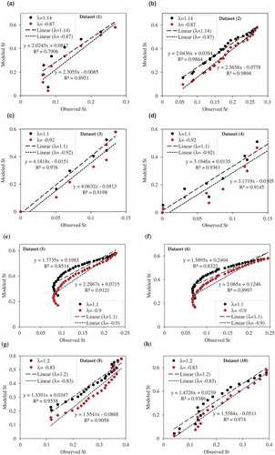
One of the key parameters in the entropy approach is the Lagrange multiplier. Determining this multiplier and its modification has a significant effect on the predicted parameter. In the regression diagrams presented in Figure 3, the estimated transverse slope is plotted against the corresponding observational values for the two values of λ obtained from the numerical solution of Equations (16) and (15). From the solution of these two equations for each observational dataset, two different negative and positive multipliers λ are obtained (referred to as modified Shannon-1 and modified Shannon-2 models, respectively), and these are used to predict the transverse slope values. The transverse slope values are then compared with the corresponding observational S_t values. It may be noted in Figure 3 that, in each set of experiments involving a channel under various hydraulic conditions, the values of λ obtained by numerical solution of the modified Shannon entropy equation are almost equal. For example, in datasets 3 and 4, which are related to the observational values of Mikhailova et al. (1980), the λ values obtained are equal to 1.1 and −0.92; the same values were obtained for the two observational datasets related to Hassanzadeh et al. (2014). For the four observational datasets of Khodashenas (2016), the identical conditions were repeated, but the results of only two observational datasets from this researcher are presented (datasets 8 and 10). The same trend was repeated for the rest of the data. Also, it is noteworthy that, for almost all observational data (10 existing observational datasets), the obtained values for multiplier λ are approximately equal, so that one of the values obtained for this multiplier is in the range of 1.1 to1.2 and the other in −0.9 to −0.83. It can be said that one of the values of λ is equal to 1 and the other is −1 approximately. When the value of λ is 1 or −1, the equation obtained by Shannon entropy is, respectively, given as follows:

(25) $S_{\mathrm{t}}=ln\left[1+(\mathrm{e}\mathrm{x}\mathrm{p}(\mu )-1)\frac{x}{L}\right]\lambda \approx 1$(25)

(26) $S_{\mathrm{t}}=-ln\left[1+(\mathrm{e}\mathrm{x}\mathrm{p}(-\mu )-1)\frac{x}{L}\right]\lambda \approx -1$(26)

Figure 3. Regression diagrams of transverse slope (S_t) predicted by the modified Shannon entropy model in comparison with the corresponding observational values for the 10 study datasets: (a) Ikeda (1981); (b) Diplas (1990); (c) Mikhailova et al. (1980) dataset 1; (d) Mikhailova et al. (1980) dataset 2; (e) Hassanzadeh et al. (2014) dataset 1; (f) Hassanzadeh et al. (2014) dataset 2; (g) Khodashenas (2016) dataset 2; and (h) Khodashenas (2016) dataset 4.

To verify Equations (25) and (26), the transverse slope of the channel can be estimated and compared with the observational values. It is found that the analysis expressed on the basis of the concept of probability in entropy is enormously influenced by the multiplier λ (Chembolu and Dutta 2018). Sterling and Knight (2002) also pointed out the marked effect of multiplier λ on shear stress estimation. Thus, the physical concept can be attributed to the amount of this multiplier (Cao and Knight 1997).

The obvious issue in examining the stability of channels is to determine in what way the channel is stable (Hassanzadeh et al. 2014). For example, Pizzuto (1990) defined the equilibrium condition for stable channels as a stable cross-section, which is obtained when there is channel widening and bank erosion. He did not restrict the motion of sediment particles and stated that there is the probability of a small sediment transport rate. In contrast, according to the initial definition of the stable channel by Glover and Florey (1951) and Lane (1955), the condition of channel equilibrium is considered to be zero sediment transport rate across the channel. The transfer of sediment particles in the bed and any other part of the channel is not in accordance with the initial definition of the channel stability condition. Thus, Parker (1978) refers to the “stable channel paradox”, and the eddy diffusion due to turbulence is considered as the cause of lateral momentum transfer and as a consequence of the shear stress redistribution. Therefore, the channel is stable when the shear stress in the channel banks is less than or equal to the critical shear stress. So, if the difference between these two shear stresses is zero, the channel is in the threshold state, which is the subject of the present study based on the theory of entropy. In fact, the stable criterion (reaching a stable state) is the zero difference between exiting and critical shear stresses (Cao and Knight 1997, Yu and Knight 1998, Dey 2001, Khodashenas 2016). Therefore, according to the channel stability assessment criteria mentioned, the physical concept of λ can be expressed as:

(27) $\lambda =\eta {\tau }^{\ast }\pm 1$(27)

where η is the experimental and laboratory coefficient and τ* is the dimensionless shear stress of the channel (Shields parameter), which is expressed as:

(28) ${\tau }^{\ast }=\left(\frac{{\tau }_{\mathrm{a}}-{\tau }_{\mathrm{c}}}{{\tau }_0}\right)$(28)

where τ_a, τ_c and τ₀ correspond, respectively, to actual shear stresses in the points on the channel banks, critical shear stress and shear stress in the channel bed. When the value of τ* is zero, λ is equal to ±1, which are the values of λ obtained by Equation (15). The physical concept expressed for λ in this study is based on the shear stress distribution (Yu and Knight 1998, Dey 2001, Karmaker and Dutta 2011). The main difference between this study and that of Cao and Knight (1997) is to provide a solvable equation for the multiplier λ, and, according to the available observable values, different values for λ might be obtained (Equation (15)), referred to herein as the modified Shannon entropy theory. In this case, it is no longer necessary to test the transverse slope of the channel based on a certain range of λ values, and it is possible to calculate the value of λ directly.

In the following, the predicted S_t values (using Equation (16)), based on these two multipliers (Fig. 3) are evaluated. In Table 3, the error indices for each λ multiplier related to observational data are shown in the prediction of the channel transverse slope. It may be seen in Figure 3 that both models of modified Shannon 1 and 2 (different λs) perform well in predicting the transverse slope of the channel with an acceptable determination coefficient (R²) for all observational datasets. Based on the equation of curvature (fitted as y = ax + b and presented in each graph), it is clear that for most datasets R² is approximately equal to one. The R² in all datasets is between 0.85 and 0.9, which indicates the acceptable performance of the proposed model based on the modified Shannon entropy concept. The lowest accuracy is in datasets 5 and 6 with R² of 0.8, which increases to 0.91 for a negative value of λ. Also, it may be seen from Table 3 that the error values for S_t predicted by the modified Shannon-1 entropy with positive values of λ are greater than the error values of the modified Shannon-2 entropy with negative value of λ. It is also observed that, for all observational data, the values of MARE, RMSE and Bias for positive λ values (1–1.2) are greater than the corresponding values of the error index for negative values of λ. Therefore, it can be concluded that the modified Shannon entropy better estimates the transverse slope of the channel based on negative λ values.

Table 3. Error index values obtained for the transverse slope predicted by different models in comparison with the corresponding observational values in different datasets.

Model	Modified Shannon-1			Modified Shannon-2			Cao and Knight (1997)
λ range	λ = −0.9 to −0.83			λ = 1 to 1.2			-
Dataset No.	MARE	RMSE	Bias	MARE	RMSE	Bias	MARE	RMSE	Bias
(1)	1.303	0.203	0.170	1.783	0.246	0.221	1.611	0.250	0.12
(2)	0.876	0.190	0.170	1.217	0.236	0.227	1.060	0.212	0.195
(3)	1.956	0.260	0.212	2.523	0.300	0.260	2.220	0.28	0.24
(4)	4.265	0.211	0.160	7.017	0.246	0.205	5.325	0.227	0.180
(5)	1.856	0.260	0.250	2.330	0.310	0.305	2.097	0.284	0.276
(6)	2.184	0.273	0.263	2.721	0.321	0.320	2.457	0.295	0.290
(8)	0.303	0.100	0.020	0.490	0.127	0.078	0.370	0.108	0.043
(10)	0.3524	0.092	0.065	0.545	0.137	0.119	0.414	0.110	0.087
Average	1.637	0.198	0.164	2.328	0.240	0.217	2.000	0.221	0.180

The MARE index for predicted transverse slope using negative values of λ shows better model performance than using positive λ with about 42% difference for the total datasets. It is also observed that in all observational data, the value of the Bias index is positive, which indicates an overestimation of the modified entropy model. This is seen in the graphs of Figure 3, in which the values predicted by the models are greater than the corresponding observational values. The best performance of the entropy model presented herein is for datasets 8 and 10 (Khodashenas 2016), which have the smallest error indices. Therefore, there is more justification for using the proposed entropy model with the Khodashenas (2016) dataset (Gholami et al. 2018c).

In addition, to evaluate the modified entropy model, the results of the Cao and Knight (1997) parabolic equation were extracted; the statistical error index of this model is also presented in Table 3. It is observed that the accuracy of the model obtained with the Cao and Knight (1997) entropy is acceptable in comparison with the two sets of predicted values for S_t with positive and negative λ values. The comparison of error values obtained from the predictions using the Cao and Knight (1997) equation with the corresponding observational values shows that their model is quite similar to the modified Shannon-1 model for positive λ values. However, the remarkable point is that the error of the Cao and Knight model is greater than that of the presented modified Shannon-1 model for negative λ values. Therefore, the accuracy of the modified entropy model using negative values of λ is greater than that of the Cao and Knight (1997) equation, and our model performs better in predicting the transverse slope of the channel.

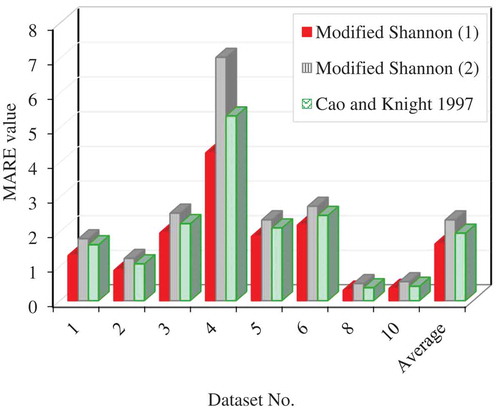
The MARE index of the modified Shannon-1 entropy model is about 22% improved compared to the previous Shannon equation by Cao and Knight (1997). Figure 4 shows a bar graph of the MARE relative error index between the transverse slope values predicted by the modified Shannon entropy model for both positive and negative values of λ and the Cao and Knight (1997) model compared to the corresponding observational values for the 10 datasets used. It may be observed from Figure 4 that the shortest column out of all the observational data is related to the modified Shannon-1 model with negative λ values, which has smaller errors than the other two models (modified Shannon-1 and Cao and Knight 1997). As in the sets of mean error values for all datasets, the difference between this model and the other two models is quite marked.

Figure 4. Bar graph of MARE for predicted transverse slope obtained by the modified Shannon entropy model with two negative and positive values of λ and the Cao and Knight (1997) relationship.

Therefore, it can be said that the equation presented in this study is more accurate with less error in the prediction of the transverse slope of stable channels and it may be introduced as a new and superior equation for predicting bank profile S_t. The notable advantage is the demonstration of a solvable relationship for λ, which has not been done in previous studies. Moreover, the mentioned arguments for the physical concept of the parameter λ are completely correct and consistent with the observational values and the initial principles of stable channels. Equation (27) is therefore proposed as the equation for determining the values of Lagrange multipliers and details are provided as to the evaluation of these multipliers.

3.2 New relationships for calculating λ

In the previous section, the relationship provided by Cao and Knight (1997) and the modified Shannon entropy model presented herein were investigated using positive and negative values of λ. To evaluate the λ multipliers accurately in the prediction of the transverse slope of stable channels, the effective parameters for the values of this multiplier and their individual effects are next discussed in detail numerically. Finally, a more accurate relationship with less error for λ is presented and evaluated. The results of evaluating the different input parameters and modelling process explained in Section 2.3 are presented.

From Figure 5 and Table 4, it is observed that Model 5 is the most accurate model in the prediction of λ, with the lowest MARE and RMSE of 0.070 and 0.039, respectively, and inputs d₅₀/h_c, x/L and SN/SX. Therefore, it can be said that the presence of these three input parameters has a significant effect on the calculation of this multiplier. Then, it can be seen that Model 1, in which all four parameters (Fr_m, d₅₀/h_c, x/L, SN/SX) are used as input, has a small error value, so it is more efficient than other models due to the presence of all input parameters. Comparison of Models 5 and 8 shows that the absence of the x/L parameter resulted in an increase in the error of Model 8, so a significant effect of that input parameter (x/L) can be noted in the prediction of λ. However, comparison of Models 5 and 11 shows that, with the lack of input parameter d₅₀/h_c in Model 11, the performance of that model with only two inputs (x/L and SN/SX) is not significantly different from that of Model 5 with all three input parameters. The error values are approximately the same, and the performance of Model 11 is also acceptable.

Table 4. Evaluation of Models 1–15 presented in this study based on different inputs using different statistical indices.

Model no.	Input variables	MARE	RMSE	Bias
1	Frm, d50/hc, x/L, SN/SX	0.071	0.039	0.0021
2	Frm, d50/hc, x/L	0.077	0.041	0.0028
3	Frm, d50/hc, SN/SX	0.148	0.082	−0.0016
4	Frm, x/L, SN/SX	0.074	0.040	0.0024
5	d50/hc, x/L, SN/SX	0.070	0.039	0.0023
6	Frm, d50/hc	0.148	0.083	−0.0008
7	d50/hc, x/L	0.159	0.080	0.0042
8	d50/hc, SN/SX	0.148	0.082	−0.0016
9	Frm, x/L	0.130	0.070	0.0042
10	Frm, SN/SX	0.172	0.092	–0.0001
11	x/L, SN/SX	0.085	0.046	0.0027
12	Frm	0.230	0.120	1.38E-05
13	d50/hc	0.254	0.127	0.0006
14	x/L	0.159	0.080	0.0042
15	SN/SX	0.172	0.092	−0.0001

The comparison of Models 4 and 5 with Model 1 shows that the removal of one of the parameters Fr_m and d₅₀/h_c has no significant effect on the error index value, and the performances of all three models is quite similar. As may be seen in the bar graphs in Figure 6, the error index for models 4, 5 and 1 is approximately equal. The reason for this is the presence of the two effective parameters x/L and SN/SX in these models. With careful evaluation of Models 7 and 8, the impressive impact of these two parameters may be seen. By eliminating one of these parameters, the performance of the model is greatly weakened, especially for Model 8, where the weakness is greater than in Model 7; the cause is a significant effect of the x/L parameter. The scatter plot diagrams of Figure 5 for both Models 7 and 8 confirm this; the compression of the values around the exact line in Model 7 is greater than in Model 8 and the poor performance of Model 8 is seen, especially in the training stage. Also, from comparison of Models 2 and 3 with Model 1, it is seen that the error of Model 3 is smaller than that of Model 1 (with all input parameters) due to the lack of parameter x/L, compared to Model 2 (which lacked SN/SX); therefore, the effect of this geometric parameter (x/L) on the prediction of λ is significant.

Figure 5. Evaluation of the correlation λ values predicted by the numerical model proposed in this study compared to the corresponding observational values in Models 1–15.

Figure 5. Continued.

Figure 5. Continued.

Some researchers, such Hey and Thorne (1986), Lee and Julien (2006), Karmaker and Dutta (2015), Yousefi et al. (2016), have pointed out the impressive effect of channel slope in river banks. In this study, that issue can be confirmed by the single-input models. For example, Model 14, which has only the x/L parameter, has an acceptable error (MARE = 0.1587, R² = 0.607) and has the best performance compared to the other single-parameter input models. Comparison of Model 14 with Model 15, with only the SN/SX parameter, shows the greater effect of the x/L parameter in the slightly higher error index values (MARE = 0.172, R² = 0.478). This is seen in Figure 5, in which the scattering of the predicted values in Model 15 is much higher than that of Model 14, while in Model 14 the compression of the values around the exact line is clearly seen.

Regarding the performance of Models 12 and 13, the negligible impact of the parameters Fr_m and d₅₀/h_c for the value prediction of λ can be noted; the error index values in these two models are about 25%, which is much more significant than for the other models (14 and 15). Also, in Figure 6, the highest error column is related to Models 12 and 13. This can also be interpreted in the graphs of Figure 5, in which the predicted λ values are approximately the same for all observational values as the data are distributed along a horizontal line, and the performance of the models is very weak. Particularly in Model 13 (input parameter d₅₀/h_c), this accuracy reduction is more than for Model 12; the estimated exact line for values in Model 12 is slightly oblique to the horizontal, while for Model 13 the line is completely horizontal. Therefore, it can be said that the presence of the parameter Fr_m, which represents different values of the discharge flow rate in each observational dataset, is more effective than that of parameter d₅₀/h_c, which indicates the sediment with a different particle diameter, in predicting the values of the λ multiplier (Eaton et al. 2004, Xu 2004, Lee and Julien 2006, Afzalimehr et al. 2010). The comparison between Models 7 and 9 also confirms this: although the value of the model error index is increased due to the presence of the x/L parameter, it is observed that the presence of Fr_m in Model 9 compared to d₅₀/h_c in Model 7 makes it more efficient, with a lower error value in Model 9.

Figure 6. Bar charts of MARE for Models 1–15 with different input combinations to predict the multiplier λ in the modified Shannon entropy equation.

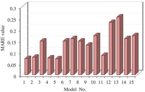
Violations of this issue are seen in Models 8 and 10, however. This is because the error value of Model 8, with the presence of the d₅₀/h_c parameter, is lower than that of Model 10 (with the Fr_m parameter). To clarify this, a more detailed comparison of Models 4 and 5 with Model 1 was made. As shown above, removing one of the parameters Fr_m and d₅₀/h_c from Models 4 and 5 did not change the model performance much compared to Model 1, due to the presence of the more effective parameters x/L and SN/SX However, in Model 4, the error index values are slightly increased compared to Model 1; the performance of Model 4 is slightly weaker compared to Model 5, which has improved performance compared to Model 1, with a decreased error index. Therefore, it can be said the performance of Model 5 is better than that of Model 4, indicating that the effect of the parameter d₅₀/h_c in combination with the two main parameters x/L and SN/SX, compared to the effect of the parameter Fr_m, is greater. In general, it can be concluded that Model 5, with the highest correlation coefficient and the smallest error index, performs more accurately than all the other models. Model 1, with all the parameters present, was selected as the second-best model. The influence of parameters Fr_m and d₅₀/h_c on the prediction of the multiplier λ was found to be negligible.

Moreover, the presence of all input parameters, or even three among the four existing parameters, causes chaos in the extraction of a relationship from the model. Therefore, Model 11, which uses the two important parameters x/L and SN/SX, is selected as the best model in this study. The multiplier λ is related to the geometric parameters x/L and SN/SX, but the properties of materials used during the channel’s stabilization, which are also contained in the SX parameter (μ), are also effective. Therefore, the relationships of four models – 11, 5, 1 and 14 – are presented in Table 5. The relationship of Model 5 is presented as the best model with the highest accuracy and the least error of all the models; the Model 1 relationship is presented, as it uses all four parameters, but is also the most accurate after Model 5; and the Model 14 relationship is presented due to the significant effect of the x/L parameter. Finally, the relationship of Model 11, as the relationship introduced in the present study, is presented for prediction of the multipliers λ in the presence of the two parameters x/L and SN/SX.

Table 5. Equations found by this study as the best performing models for predicting the value of the multiplier λ based on the entropy concept. See Table 4 for input variables in each model.

Model no.	Presented relation
11	$\lambda =0.0838(\frac{\mathrm{S}\mathrm{N}}{\mathrm{S}\mathrm{X}})-0.5665(\frac{x}{L})+0.0279\left((\frac{x}{L})/(\frac{SN}{SX})\right)+0.7835$
5	$\begin{array}{c}\lambda =0.5949(\frac{d_{50}}{{\mathrm{h}}_c})(\frac{SN}{SX})+0.0254\left((\frac{x}{L})/(\frac{\mathrm{S}\mathrm{N}}{\mathrm{S}\mathrm{X}})\right)-0.0225\left((\frac{x}{L})/(\frac{d_{50}}{{\mathrm{h}}_c})\right)+\\ 0.0362\left(1/(\frac{d_{50}}{h_c})\right)-0.4415(\frac{x}{L})-0.3075(\frac{\mathrm{S}\mathrm{N}}{\mathrm{S}\mathrm{X}})+0.6284\end{array}$
1	$\begin{array}{c}\lambda =-0.4554(\frac{x}{L})(\frac{\mathrm{S}\mathrm{N}}{\mathrm{S}\mathrm{X}})+0.0216\left(1/(\frac{d_{50}}{{\mathrm{h}}_c})\right)+0.0092\left(1/(\frac{SN}{SX})\right)+0.1833(\frac{d_{50}}{h_c})-\\ 0.2736(\frac{x}{L})+0.5529\end{array}$
14	$\lambda =-0.4661(\frac{x}{L})+0.7861$

4 Uncertainty analysis

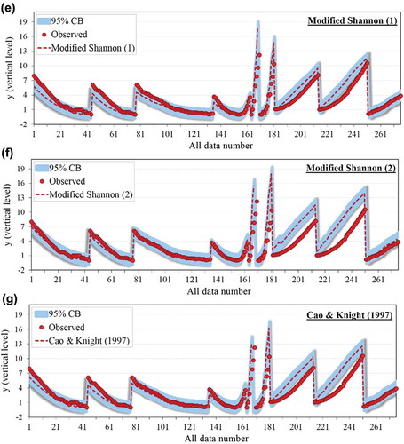
In this section, the uncertainty of EPR models 1, 5, 11 and 14 in estimating the entropy parameter (λ) is analysed. Table 6 presents the uncertainty indexes for the EPR and entropy models in the training and testing stages. The λ values estimated by the EPR model and the vertical boundary level (y) predicted by the modified Shannon entropy models and the Cao and Knight (1997) relationship, as well as the 95% CB are presented in Figure 7 and Table 6. As may be seen in Figure 7, the four EPR models (1, 5, 11 and 14) can well estimate λ, having high conformity with observed values.

Table 6. Uncertainty analysis and indices of the EPR models 1, 5, 11 and 14 for the prediction of entropy parameter (λ) and the modified Shannon-1 and -2 and Cao and Knight (1997) entropy models.

Model	Dataset	No of samples	MPE	Se	WCB	95% CB
EPR models
Model 1	Training	206	0.03	0.027	±0.0037	+0.026 to +0.033
	Test	68	0.029	0.027	±0.0064	+0.023 to +0.036
Model 5	Training	206	0.028	0.027	±0.0037	+0.025 to +0.032
	Test	68	0.028	0.026	±0.0064	+0.022 to +0.0350
Model 11	Training	206	0.035	0.030	±0.0042	+0.030 to +0.039
	Test	68	0.035	0.030	±0.0072	+0.028 to +0.042
Model 14	Training	206	0.062	0.045	±0.0062	+0.056 to +0.069
	Test	68	0.065	0.047	±0.0114	+0.054 to +0.076
Entropy models
Modified Shannon-1	All	276	0.960	1.133	±0.134	+0.825 to +1.094
Modified Shannon-2	All	276	1.105	1.410	±0.167	+0.938 to +1.272
Cao and Knight (1997)	All	276	1.084	1.393	±0.165	+0.919 to +1.249

Figure 7. The 95% CB ranges for predicted entropy parameter (λ) using EPR models: (a) Model 1, (b) Model 2, (c) Model 11 and (d) Model 14, and estimated vertical level (y) of points located on stable channel banks using the entropy models (e) modified Shannon-1, (f) modified Shannon-2 and (g) Cao and Knight (1997).

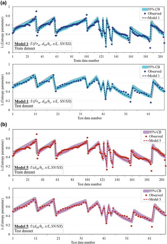
Figure 7. Continued.

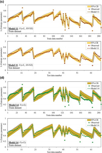
Figure 7. Continued.

The MPE and S_e values (Table 6) confirm this observation, and all four EPR models have MPE values in the range of 2–6% in both training and testing stages, indicating the acceptable accuracy of the EPR models in λ estimation. Furthermore, the WCB value for EPR models 1, 5, 11 and 14 is very small, as indicated by the narrow confidence bounds in Figure 7. The low WCB and small error index values for these models represent low uncertainty, or greater reliability of the EPR models in estimating λ. The 95% CB values for all four models are also presented in Table 6. As seen from the MPE and WCB values, Model 5, with the lowest MPE of 0.0286 and WCB of ±0.0064 in the testing stage, has the lowest uncertainty compared to other models and estimates λ with more accuracy. However, Model 1 has acceptable accuracy, only slightly different from Model 5, while Model 14, with higher MPE and WCB, is less reliable compared to the other models. The simultaneous effect of parameters d₅₀/h_c, x/L and SN/SX on model performance is a significant issue in the estimation of entropy parameter λ. Overall, the low values of uncertainty indexes for the EPR models obtained in this study indicate higher accuracy and greater reliability of the proposed models.

The uncertainty indexes for the modified Shannon-1 and -2 entropy models proposed in this study and the relationship proposed by Cao and Knight (1997) are also presented in Table 6. It may be seen that the modified Shannon-1 model has the lowest MPE and S_e (0.960 and 1.133, respectively), which indicates higher accuracy of this model compared to the Cao and Knight (1997) relationship. The modified Shannon-1 model also has the lowest WCB (±0.134) compared to the modified Shannon-2 and the Cao and Knight (1997) models (±0.167 and ±0.165, respectively), which is clearly seen in the narrow CB range of this model in Figure 7, Therefore, it can be concluded that the entropy model proposed in this paper leads to more accurate results and less uncertainty (i.e. greater reliability).

5 Conclusions

A comprehensive study of the transverse slope of stable channel banks based on a novel application of the entropy theory was carried out to provide new insights into a complex hydraulic problem. The new equations were obtained based on the principle of maximum entropy, which governs the probability distribution of stable river bank profiles. Based on this fundamental principle, an equation for calculating the entropy parameter (λ) is presented, with its numerical solution for 10 datasets. The corresponding equation for λ can be used together with the equation of the channel transverse slope in the estimation of the slope of a stable channel.

By obtaining an observational value of λ for each point along the stable profile boundary of a river bank, the influence of factors affecting this multiplier, such as the modified Froude number (Fr_m), the average dimensionless particle size (d₅₀/h_c), the dimensionless transverse interval (x/L = x*) and the ratio of maximum slope to average slope of the bank (SN/SX) was investigated using a numerical model, and a relationship is presented for calculating λ based on these multipliers. A formula to calculate the values of λ based on two parameters (x/L and SN/SX) is introduced in this research as the proposed relationship since it gave smaller errors compared to the other relationships of the other models. Accordingly, the multiplier λ is related to the geometric parameters x/L and SN/SX, but the properties of materials used in the stabilization of a channel, which are also contained in the SX parameter (μ), are also effective. Furthermore, the uncertainty results demonstrated the greater reliability of EPR models 1, 5, 11 and 14, which had the smallest WCB (±0.0064, ±0.0064, ±0.0072 and ±0.0114, respectively) compared to the other models. Also, the modified Shannon entropy model proposed in this study (WCB and MPE of ±0.134 and 0.960, respectively) is shown to be more accurate and reliable than the relationship proposed by Cao and Knight (1997) based on Shannon entropy, with WCB and MPE of ±0.165 and 1.084, respectively. The numerical-based relationship presented here can be used based on the physical concept of λ, as well as the equation provided by the entropy principle, to calculate the value of λ and, therefore, the transverse slope of the stable channel bank profile and the vertical boundary level. Finally, the results of the relationships presented in this study were compared with the previous relationships based on different theories.

Disclosure statement

No potential conflict of interest was reported by the authors.

References

- Afzalimehr, H., Abdolhosseini, M., and Singh, V.P., 2010. Hydraulic geometry relations for stable channel design. Journal of Hydrologic Engineering, 15 (10), 859–864. doi:10.1061/(ASCE)HE.1943-5584.0000260
- Atieh, M., et al., 2017. Prediction of flow duration curves for ungauged basins. Journal of Hydrology, 545, 383–394. doi:10.1016/j.jhydrol.2016.12.048
- Atieh, M., Gharabaghi, B., and Rudra, R., 2015. Entropy-based neural networks model for flow duration curves at ungauged sites. Journal of Hydrology, 529 (3), 1007–1020. doi:10.1016/j.jhydrol.2015.08.068
- Bender, R., 2001. Calculating confidence intervals for the number needed to treat. Controlled Clinical Trials, 22 (2), 102–110.
- Berry, G. and Armitage, P., 1995. Mid-P confidence intervals: a brief review. Journal of the Royal Statistical Society. Series D (The Statistician), 44 (4), 417–423.
- Bonakdari, H., 2012. Establishment of relationship between mean and maximum velocities in narrow sewers. Journal of Environmental Management, 113, 474–480. doi:10.1016/j.jenvman.2012.10.016
- Bonakdari, H. and Gholami, A., 2016. Evaluation of artificial neural network model and statistical analysis relationships to predict the stable channel width. River Flow 2016: Iowa City, USA, July 11–14: 417.
- Bonakdari, H., Sheikh, Z., and Tooshmalani, M., 2015. Comparison between Shannon and Tsallis entropies for prediction of shear stress distribution in open channels. Stochastic Environmental Research and Risk Assessment, 29 (1), 1–11. doi:10.1007/s00477-014-0959-3
- Cao, S. and Knight, D.W., 1997. Entropy-based design approach of threshold alluvial channels. Journal of Hydraulic Research, 35 (4), 505–524. doi:10.1080/00221689709498408
- Chembolu, V. and Dutta, S., 2018. An entropy based morphological variability assessment of a large braided river. Earth Surface Processes and Landforms, 43 (14), 2889–2896. doi:10.1002/esp.v43.14
- Chiu, C.L., 1987. Entropy and probability concepts in hydraulics. Journal of Hydraulic Engineering, 113 (5), 583–599. doi:10.1061/(ASCE)0733-9429(1987)113:5(583)
- Chiu, C.L., Hsu, S.M., and Tung, N.C., 2005. Efficient methods of discharge measurement in rivers and stream based on the probability concept. Hydrological Process, 19, 3935–3946. doi:10.1002/hyp.5857
- Chow, V.D., 1959. Open channel hydraulic. New York: McGraw-Hill.
- Cui, H. and Singh, V.P., 2013. Computation of suspended sediment discharge in open channels by combining tsallis entropy-based methods and empirical formulas. Journal of Hydrologic Engineering, 19 (1), 18–25. doi:10.1061/(ASCE)HE.1943-5584.0000782
- Dey, S., 2001. Bank profile of threshold channels: a simplified approach. Journal of Irrigation and Drainage engineering-ASCE, 127 (3), 184–187. doi:10.1061/(ASCE)0733-9437(2001)127:3(184)
- Diplas, P., 1990. Characteristics of self-formed straight channels. Journal of Hydraulic Engineering, 116 (5), 707–728. doi:10.1061/(ASCE)0733-9429(1990)116:5(707)
- Diplas, P. and Vigilar, G., 1992. Hydraulic geometry of threshold channels. Journal of Hydraulic Engineering, 118 (4), 597–614. doi:10.1061/(ASCE)0733-9429(1992)118:4(597)
- Eaton, B. and Millar, R., 2017. Predicting gravel bed river response to environmental change: the strengths and limitations of a regime‐based approach. Earth Surface Processes and Landforms, 42 (6), 994–1008. doi:10.1002/esp.v42.6
- Eaton, B.C., Church, M., and Millar, R.G., 2004. Rational regime model of alluvial channel morphology and response. Earth Surface Processes and Landforms, 29, 511–529. doi:10.1002/esp.v29:4
- Ebtehaj, I., Bonakdari, H., and Gharabaghi, B., 2019. A reliable linear method for modeling lake level fluctuations. Journal of Hydrology, 570, 236–250. doi:10.1016/j.jhydrol.2019.01.010
- Gholami, A., et al., 2016a. Improving the performance of multi-layer perceptron and radial basis function models with a decision tree model to predict flow variables in a sharp 90° bend. Applied Soft Computing, 48, 563–583. doi:10.1016/j.asoc.2016.07.035
- Gholami, A., et al., 2016b. Design of modified structure multi-layer perceptron networks based on decision trees for the prediction of flow parameters in 90° open-channel bends. Engineering Applications of Computational Fluid Mechanics, 10 (1), 193–208. doi:10.1080/19942060.2015.1128358
- Gholami, A., et al., 2017a. Developing an expert group method of data handling system for predicting the geometry of a stable channel with a gravel bed. Earth Surface Processes and Landforms, 42 (10), 1460–1471. doi:10.1002/esp.v42.10
- Gholami, A., et al., 2017b. Design of an adaptive neuro-fuzzy computing technique for predicting flow variables in a 90° sharp bend. Journal of Hydroinformatics, 19 (4), 572–585. doi:10.2166/hydro.2017.200
- Gholami, A., et al., 2018a. Reliable method of determining stable threshold channel shape using experimental and gene expression programming techniques. Neural Computing and Applications, 1–19. doi:10.1007/s00521-018-3411-7
- Gholami, A., et al., 2018b. New radial basis function network method based on decision trees to predict flow variables in a curved channel. Neural Computing and Applications, 30 (9), 2771–2785. doi:10.1007/s00521-017-2875-1
- Gholami, A., et al., 2018c. A methodological approach of predicting threshold channel bank profile by multi-objective evolutionary optimization of ANFIS. Engineering Geology, 239, 298–309. doi:10.1016/j.enggeo.2018.03.030
- Gholami, A., et al., 2018d. Uncertainty analysis of intelligent model of hybrid genetic algorithm and particle swarm optimization with ANFIS to predict threshold bank profile shape based on digital laser approach sensing. Measurement, 121, 294–303. doi:10.1016/j.measurement.2018.02.070
- Gholami, A., et al., 2019. A comparison of artificial intelligence-based classification techniques in predicting flow variables in sharp curved channels. Engineering with Computers, 1–30. doi:10.1007/s00366-018-00697-7
- Giustolisi, O. and Savic, D.A., 2006. A symbolic data-driven technique based on evolutionary polynomial regression. Journal of Hydroinformatics, 8, 207–222. doi:10.2166/hydro.2006.020b
- Giustolisi, O. and Savic, D.A., 2009. Advances in data-driven analyses and modelling using EPR-MOGA. Journal of Hydroinformatics, 11, 225–236. doi:10.2166/hydro.2009.017
- Glover, R.E. and Florey, Q.L., 1951. Stable channel profiles. Lab. Rep. 325Hydraul. Washington, DC: U.S. Bureau of Reclamation.
- Hassanzadeh, Y., et al., 2014. Validation of river bank profiles in sand-bed rivers. Journal of Civil and Environmental Engineering, 43 (4), 59–68.
- Hey, R.D. and Thorne, C.R., 1986. Stable channels with mobile gravel beds. Journal of Hydraulic Engineering, 112 (8), 671–689. doi:10.1061/(ASCE)0733-9429(1986)112:8(671)
- Huang, H.Q., et al., 2014. A test of equilibrium theory and a demonstration of its practical application for predicting the morphodynamics of the Yangtze River. Earth Surface Processes and Landforms, 39 (5), 669–675. doi:10.1002/esp.v39.5
- Ikeda, S., 1981. Self-formed straight channels in sandy beds. Journal of Hydraulic Division ASCE, 107, 389–406.
- Ikeda, S., Parker, G., and Kimura, Y., 1988. Stable width and depth of straight gravel rivers with heterogeneous bed materials. Water Resources Research, 24, 713–722. doi:10.1029/WR024i005p00713
- Joshi, I., et al., 2018. Evaluation and comparison of extremal hypothesis-based regime methods. Water, 10 (3), 271. doi:10.3390/w10030271
- Jowitt, P.W., 1991. A maximum entropy view of probability-distributed catchment models. Hydrological Sciences Journal, 36 (2), 123–134. doi:10.1080/02626669109492494
- Julien, P.Y., 2015. Downstream hydraulic geometry of alluvial rivers. Proceedings of the International Association of Hydrological Sciences, 367, 3–11. doi:10.5194/piahs-367-3-2015
- Kaless, G., Mao, L., and Lenzi, M.A., 2014. Regime theories in gravel‐bed rivers: models, controlling variables, and applications in disturbed Italian rivers. Hydrological Processes, 28 (4), 2348–2360. doi:10.1002/hyp.9775
- Karmaker, T. and Dutta, S., 2011. Erodibility of fine soil from the composite river bank of Brahmaputra in India. Hydrological Processes, 25 (1), 104–111. doi:10.1002/hyp.7826
- Karmaker, T. and Dutta, S., 2015. Stochastic erosion of composite banks in alluvial river bends. Hydrological Processes, 29 (6), 1324–1339. doi:10.1002/hyp.v29.6
- Khodashenas, S.R., 2016. Threshold gravel channels bank profile: a comparison among 13 models. International Journal of River Basin Management, 14 (3), 337–344. doi:10.1080/15715124.2016.1170693
- Khozani, Z.S. and Bonakdari, H., 2018. Formulating the shear stress distribution in circular open channels based on the Renyi entropy. Physica A: Statistical Mechanics and Its Applications, 490, 114–126. doi:10.1016/j.physa.2017.08.023
- Kumbhakar, M., Kundu, S., and Ghoshal, K., 2017. Hindered settling velocity in particle-fluid mixture: a theoretical study using the entropy concept. Journal of Hydraulic Engineering, 143 (11), 06017019. doi:10.1061/(ASCE)HY.1943-7900.0001376
- Kundu, S., 2018. Derivation of different suspension equations in sediment-laden flow from Shannon entropy. Stochastic Environmental Research and Risk Assessment, 32 (2), 563–576. doi:10.1007/s00477-017-1455-3
- Lane, E.W., 1955. Design of stable channels. Trans. ASCE, 120, 1234–1260.
- Lee, J.S. and Julien, P.Y., 2006. Downstream hydraulic geometry of alluvial channels. Journal of Hydraulic Engineering, 132, 1347–1352. doi:10.1061/(ASCE)0733-9429(2006)132:12(1347)
- Liu, D., et al., 2017. Complexity measure of regional seasonal precipitation series based on wavelet entropy. Hydrological Sciences Journal, 62 (15), 2531–2540. doi:10.1080/02626667.2017.1390313
- Luo, H. and Singh, V.P., 2011. Entropy theory for two-dimensional velocity distribution. Journal of Hydrologic Engineering, 16 (4), 725–735. doi:10.1061/(ASCE)HE.1943-5584.0000319
- Métivier, F., Lajeunesse, E., and Devauchelle, O., 2017. Laboratory rivers: lacey‘s law, threshold theory, and channel stability. Earth Surface Dynamics, 5 (1), 187–198. doi:10.5194/esurf-5-187-2017
- Mikhailova, N.A., Shevchenko, O.B., and Selyametov, M.M., 1980. Laboratory investigation of the formation of stable canal channels. Hydro Technical Construction, 14, 714–722. doi:10.1007/BF02305503
- Millar, R.G., 2005. Theoretical regime equations for mobile gravel-bed rivers with stable banks. Geomorphology, 64 (3–4), 207–220. doi:10.1016/j.geomorph.2004.07.001
- Moramarco, T. and Singh, V.P., 2010. Formulation of the entropy parameter based on hydraulic and geometric characteristics of river cross sections. Journal of Hydrologic Engineering, 15 (10), 852–858. doi:10.1061/(ASCE)HE.1943-5584.0000255
- Nanson, G.C. and Huang, H.Q., 2018. A philosophy of rivers: equilibrium states, channel evolution, teleomatic change and least action principle. Geomorphology, 302 (1), 3–19. doi:10.1016/j.geomorph.2016.07.024
- Parker, G., 1978. Self-formed straight rivers with equilibrium banks and mobile bed, Part 2. The gravel river. Journal of Fluid Mechanics, 89 (1), 127–146. doi:10.1017/S0022112078002505
- Pechlivanidis, I.G., et al., 2016. Robust informational entropy-based descriptors of flow in catchment hydrology. Hydrological Sciences Journal, 61 (1), 1–18. doi:10.1080/02626667.2014.983516
- Pizzuto, J.E., 1990. Numerical simulation of gravel river widening. Water Resources Research, 26, 1971–1980. doi:10.1029/WR026i009p01971
- Shaghaghi, S., et al., 2017. Comparative analysis of GMDH neural network based on genetic algorithm and particle swarm optimization in stable channel design. Applied Mathematics and Computation, 313, 271–286. doi:10.1016/j.amc.2017.06.012
- Shaghaghi, S., et al., 2018a. Predicting the geometry of Regime Rivers using M5 model tree, multivariate adaptive regression splines and least square support vector regression methods. International Journal of River Basin Management, 1–20. doi:10.1080/15715124.2018.1546731
- Shaghaghi, S., et al., 2018b. Stable alluvial channel design using evolutionary neural networks. Journal of Hydrology, 566, 770–782. doi:10.1016/j.jhydrol.2018.09.057
- Shannon, C.E., 1948. A mathematical theory of communication. Bell System Technical Journal, 27, 623–656. doi:10.1002/bltj.1948.27.issue-4
- Silva, V.D.P.R.D., et al., 2017. Entropy theory for analysing water resources in northeastern region of Brazil. Hydrological Sciences Journal, 62 (7), 1029–1038.
- Singh, V.P., 2003. On the theories of hydraulic geometry. International Journal of Sediment Research, 18, 196–218.
- Sterling, M. and Knight, D.W., 2002. An attempt at using the entropy approach to predict the transverse distribution of boundary shear stress in open channel flow. Stochastic Environmental Research and Risk Assessment, 16 (2), 127–142. doi:10.1007/s00477-002-0088-2
- Vigilar, G. and Diplas, P., 1997. Stable channels with mobile bed: formulation and numerical solution. Journal of Hydraulic Engineering, 123 (3), 189–199. doi:10.1061/(ASCE)0733-9429(1997)123:3(189)
- Vigilar, G. and Diplas, P., 1998. Stable channels with mobile bed: model verification and graphical solution. Journal of Hydraulic Engineering, 124, 1097–1108. doi:10.1061/(ASCE)0733-9429(1998)124:11(1097)
- Wallis, S., 2013. Binomial confidence intervals and contingency tests: mathematical fundamentals and the evaluation of alternative methods. Journal of Quantitative Linguistics, 20 (3), 178–208. doi:10.1080/09296174.2013.799918
- Xu, J., 2004. Comparison of hydraulic geometry between sand- and gravel-bed rivers in relation to channel pattern discrimination. Earth Surface Processes and Landforms, 29 (5), 645–657. doi:10.1002/(ISSN)1096-9837
- Yousefi, N., et al., 2016. Estimating width of the stable channels using multivariable mathematical models. Arabian Journal of Geosciences, 9 (4), 321. doi:10.1007/s12517-016-2322-0
- Yu, G. and Knight, D.W., 1998. Geometry of self-formed straight threshold channels in uniform material. Proceedings of the Institution of Civil Engineers - Water Maritime and Energy, 130 (1), 31–41. doi:10.1680/iwtme.1998.30226
- Zaji, A.H., Bonakdari, H., and Gharabaghi, B., 2018a. Reservoir water level forecasting using group method of data handling. Acta Geophysica, 66 (4), 717–730. doi:10.1007/s11600-018-0168-4
- Zaji, A.H., Bonakdari, H., and Shamshirband, S., 2018b. Standard equations for predicting the discharge coefficient of a modified high-performance side weir. Scientia Iranica, 25 (3), 1057–1069.