Trend assessment of annual instantaneous maximum flows in Turkey

ABSTRACT

A comprehensive evaluation of trends in annual instantaneous maximum flows (AIMF) from 153 gauge stations located in 26 river basins in Turkey is presented. Two traditional non-parametric trend tests, the Mann-Kendall (MK) and Spearman’s rho (SR), are used to quantify the significance of trends, while Sen’s slope method is applied to determine the magnitude of trends. The traditional tests indicate that the AIMF records of 57 stations showed statistically decreasing trends, while those of six stations showed an increasing trend. Sen’s trend method, which provides more detailed assessment of the trends in different clusters (low, medium and high), was applied to the AIMF series and the results were compared with traditional tests. Sen’s trend method indicated that all flow clusters at nine stations have increasing or decreasing trends, although no significant trend was detected by the MK and SR tests.

KEYWORDS:

• maximum flows
• trend analysis
• Mann-Kendall test
• Spearman’s rho
• Sen’s slope
• Sen’s trend method

Editor A. Castellarin Associate editor S. Kanae

1 Introduction

Climate change and variability directly affect the hydrological cycle, which in turn affects both the distribution and availability of water resources for domestic use, food production, and industrial activities, as well as other hydrology-related aspects including flood control, water quality, erosion, sediment transport and deposition, and ecosystem conservation (Dam 1999). Dixon et al. (2006) pointed out that there is a growing international perception that drought and flood frequencies have increased in magnitude and/or frequency rates. Tabari et al. (2012) also reported that the global mean surface temperature has increased by 0.6°C over the last 100 years and this could lead to regional changes in the amount and intensity of the main variables of the hydrological cycle (e.g. precipitation, streamflow, temperature). Detection of significant changes in these variables is crucial for the reason that major changes often threaten our further survival or quality of life, and major anthropogenic changes bear the moral aspect of human responsibility even if one is not directly affected by them (Radziejewski 2011). Among the main variables of the hydrological cycle, streamflow is one of the most important as it relates directly to water supply, flood control, reservoir design, navigation, irrigation, drainage, water quality, and many others (Tosunoglu 2018). Additionally, in order to manage water resources in any region/basin more efficiently and effectively, it is necessary to understand, identify and quantify the possible temporal and spatial changes in different aspects of streamflow. Hence, there has been a growing number of publications on studies evaluating the temporal and spatial changes in streamflow time series in different parts of the world. For instance, Douglas et al. (2000) investigated trends in flood and low flows of United States rivers and identified statistically no evidence of trends in flood flows, but did detect increasing trends in low flows. Wang et al. (2015) assessed trends in daily, mean seasonal and maximum and minimum flow records in China and investigated the relationship between streamflow trends and climatic indices. Abeysingha et al. (2016) analysed trends in observed streamflow data at several gauging stations in the Gomti River basin of North India, and the results showed a gradual decreasing trend of annual, monsoonal and winter seasonal streamflow from the midstream to the downstream of the river. Coch and Mediero (2016) researched trends in low flows collected at 60 gauge stations in Spain, and their findings revealed a clear general pattern of decreasing trends. There are many other studies, such as: Lins and Slack (2005), Rice et al. (2015) and Ahn and Palmer (2016) who studied rivers in the USA; Zhang et al. (2006), Zhao et al. (2010), Hu et al. (2011), Zang and Liu (2013) and Song et al. (2015) for rivers in China; Petrow and Merz (2009) and Bormann et al. (2011) for German rivers; Panda et al. (2013) and Nune et al. (2014) for Indian rivers; Masih et al. (2011), Abghari et al. (2013) and Zamani et al. (2017) for rivers in Iran; Cunderlik and Ouarda (2009) and Burn and Whitfield (2016) for Canadian rivers; Lopez-Moreno et al. (2006) for Spanish rivers; and Kahya and Kalayci (2004), Topaloglu (2006), Gumus and Yenigun (2006) and Ceribasi and Dogan (2015) for rivers in Turkey.

In the studies listed above, the researchers paid significant attention to many streamflow variables, such as maximum, mean and minimum flows. Among these variables, maximum flows (floods) may be considered as among the most important types of variable, as they are crucial for the design of flood protection and flood mitigation structures. Flooding is a highly damaging catastrophe in many areas of the world. There are various factors affecting the occurrence and variability of flooding, which is a complex and dynamic process. These factors can be extreme precipitation, change in land use, dam construction, vegetation properties and soil type. The combination of climate change and human activities has caused significant changes in flood trends in many regions around the world (Bai et al. 2016). Changes in flood trends create challenges when assessing and managing flood risk. Understanding the spatial and temporal variability of flood trends is helpful for coping with the challenges and it is an important area to investigate. Taking this into consideration, Cigizoglu et al. (2005), whose results are evaluated in the Discussion section, investigated the existence of trends in annual maximum flows, as well as mean and low flows, for 100 gauging stations located in Turkish river basins. Burn et al. (2010) investigated trends in high and low flows for 68 gauging stations in Canada and, in general, downward trends at high flows and upward/downward trends at low flows were identified. Mediero et al. (2014) determined trends in magnitude, frequency and timing of annual maximum flows at 60 gauging stations in Spain in the periods 1942–2009, 1949–2009 and 1959–2009. They found a decreasing trend in annual maximum series in all three periods, with more notable evidence in the period 1959–2009 than in 1942–2009. Bai et al. (2016) investigated possible spatial and temporal changes in annual maximum flood events in the Yellow River basin, China. Their trend results indicated that the flood data for the whole basin were dominated by decreasing trends.

In these studies, the researchers mostly implemented traditional trend tests, including the Mann-Kendall and Spearman’s rho tests, in order to assess the significance of the trends. It is worth recalling that these methods are generally used to determine monotonic trends in whole time series. However, efficient, effective and optimum management of water resources requires the identification of trends not only monotonically over the whole time period, but also with respect to whether low, medium and high values have separate trends (Sen 2017). For this purpose, an innovative trend method, based on the Cartesian coordinate system, which enables trend identification to be done distinctly for low, medium and high values, was recently introduced by Sen (2012). Furthermore, unlike other non-parametric methods, this method does not have any constraints, such as serial independence, normality of the sampling distribution and sample data length. Therefore, this trend method has gained popularity in recent years. For instance, Timbadiya et al. (2013) used both the Mann-Kendall test and the Sen method to determine the trend and probability distribution of annual maximum flows at four stations in the Tapi basin, India. The results showed that both trend methods indicated a monotonic statistically significant increasing trend for all the gauging stations studied except one. Furthermore, Haktanir and Citakoglu (2014) used the Mann-Kendall and linear regression tests to evaluate temporal changes in various annual maximum rainfall series (with durations from 5 min to 24 h) recorded in 174 gauge stations of Turkey. They also applied Sen’s trend method to some series having no increasing or decreasing trends and the findings were parallel to both Mann-Kendall and linear regression tests.

Dabanli et al. (2016) used the Mann-Kendall test and the Sen method to investigate trends in hydro-meteorological data series (precipitation, temperature, humidity, runoff) at eight gauge stations in the Ergene basin, Turkey. They found that Sen’s method determined decreasing and increasing trends in high and low categories although the Mann-Kendall test did not show a statistically significant trend in nearly the all cases. Tabari et al. (2017) suggested a modified Sen method, in conjunction with the quantile perturbation method (QPM), to evaluate decadal trends of monthly and annual flow data in Iran. They showed dominance of a decreasing trend in river flow extremes for recent years. Guclu (2018) used innovative trend analysis (ITA) and the Mann-Kendall trend test, including suggested double-ITA and triple-ITA procedures and a partial MK test, to detect trends in annual rainfall records at many stations in different regions of Turkey. He concluded that triple-ITA and Mann Kendall test approaches were useful for effective and accurate stability analysis of the time series.

The main objective of this study is to investigate possible significant changes in annual instantaneous maximum flows (AIMF) for the period 1961–2017 from 153 gauging stations uniformly distributed across 26 river basins in Turkey. Two traditional non-parametric trend tests, namely the Mann-Kendall (MK) test and Spearman’s rho (SR) test, as well as the recently proposed Sen trend method, are used to evaluate the significance of temporal trends. Sen’s slope method is also applied to calculate the magnitude of the trends. Moreover, the results of Sen’s method are compared with those of the MK and SR trend tests. The findings of this study are expected to provide preliminary information for water construction designers, to enable them to plan and manage water resources more effectively.

2 Materials and methods

2.1 Serial correlation analysis

The serial correlation structure in a dependent time series is bound to affect the ability of the MK and SR tests. To illustrate, if there is a positive serial correlation in the time series, it will increase the chance of a significant answer, even in the absence of a trend (Hamed and Rao 1998). Hence, before applying these tests for trend evaluation, the serial correlation structure should be checked. If there is a significant serial correlation in a data series, the calculation of the test statistics should be modified, or a pre-whitening method should be used to remove the effect of this correlation. In this study, the trend-free pre-whitening method (TFPW), as proposed by Yue et al. (2002), was used. The pre-whitening steps of the TFPW approach are as follows:

Step 1. The first autocorrelation coefficient (r_i) is calculated as:

(1) $r_i=\frac{\frac{1}{N-i}{\sum }_{k=1}^{N-i}\left(x_i-\bar{x}\right)(x_{k+i}-\bar{x})}{\frac{1}{N}{\sum }_{k=1}^N{\left(x_k-\bar{x}\right)}^2}\mathrm{f}\mathrm{o}\mathrm{r}i=1\to r_1$(1)

Step 2. If the absolute value of $r_1$ is smaller than the critical value of $1.96/\sqrt{N}$ at the 5% significance level, as used by Douglas et al. (2000) and Tosunoglu (2017), the data are considered to be serially independent; otherwise, they are serially dependent.

Step 3. The Q value is the magnitude of the trend in the time series and the time series are detrended by:

(2) $X_i^{\prime }=X_i-T_i=X_i-Q.ii=1,2,\dots ,N$(2)

Step 4. The r₁ value (lag-1) of the detrended time series ($X_i^{\prime }$) is calculated using Equation (1). Because the serial correlation has an effect on test statistics, the lag-1 autoregressive component (AR(1)) is removed from$X_i^{\prime }$ by:

(3) $Y_i^{\prime }=X_i^{\prime }-r_1{X}_{i-1}^{\prime }$(3)

Step 5. The calculated trend, $T_i$, is added again to time series $Y_i^{\prime }$ as follows:

(4) $Y_i=Y_i^{\prime }+T_i$(4)

Finally, both the MK and SR tests are applied to time series $Y_i$.

2.2 Mann-Kendall (MK) test

The MK test is a non-parametric test for exploring a trend in a time series without specifying the type of trend (i.e. linear or nonlinear). Mann (1945) originally applied this test and Kendall (1975) subsequently derived the test-statistic distribution. Under the null hypothesis H₀, that a series (x₁, …, x₂) comes from a population in which the random variables are independent and identically distributed (clearly, in this case no trend is present), the MK test statistic can be computed as:

(5) $S=\sum _{t_1=1}^{T-1}\sum _{t_2=t_1+1}^T\mathrm{s}\mathrm{g}\mathrm{n}\left[d\left(t_1,t_2\right)\right]$(5)

where

(6) $\mathrm{s}\mathrm{g}\mathrm{n}\left[d\left(t_1,t_2\right)\right]=\left\{\begin{array}{c}1\mathrm{i}\mathrm{f}d\left(t_1,t_2\right)>0\\ 0\mathrm{i}\mathrm{f}d\left(t_1,t_2\right)=0\\ -1\mathrm{i}\mathrm{f}d\left(t_1,t_2\right)<0\end{array}\right.$(6)

For the series (x₁, …, x₂), the difference $\left\{d\left(t_1,t_2\right)\right.=x_{t_2}-x_{t_1};t_2>\left.t_1\right\}$ between all pairs of observations is calculated. Negative differences are then assigned the value −1, while positive differences are assigned the value 1, and zero differences are assigned the value 0.

For the data length T ≥ 10, S has an approximately normal probability distribution function with the mean E(S) = 0; the variance var(S) is given as:

(7) $\mathrm{v}\mathrm{a}\mathrm{r}\left(S\right)=\frac{1}{18}T\left(T-1\right)\left(2T+5\right)$(7)

In the case of tied ranks, var(S) becomes:

(8) $\mathrm{v}\mathrm{a}\mathrm{r}\left(S\right)=\frac{T\left(T-1\right)\left(2T+5\right)-{\sum }_{i=1}^k{t}_i\left(t_i-1\right)\left(2t_i+5\right)}{18}$(8)

in which k denotes the number of tied groups and t_i is the number of observations in group i. Then, the standardized MK test statistic (Z) can be defined as:

(9) $Z=\left\{\begin{array}{c}\frac{S-1}{\sqrt{\mathrm{v}\mathrm{a}\mathrm{r}\left(S\right)}}\mathrm{i}\mathrm{f}S>0\\ 0\mathrm{i}\mathrm{f}S=0\\ \frac{S+1}{\sqrt{\mathrm{v}\mathrm{a}\mathrm{r}\left(S\right)}}\mathrm{i}\mathrm{f}S<0\end{array}\right.$(9)

A negative value of S indicates a downward trend, while a positive value indicates an upward trend. If the absolute value of the calculated Z is greater than the z_1-α/2 value of the normal distribution corresponding to significance level α, the null hypothesis (H₀) is rejected and the trend is considered statistically significant. If Z is less than z_1-α/2, H₀ is accepted, implying that there is no statistically significant trend (Yu et al. 1993).

If there is a significant autocorrelation in the considered time series, the modified Mann-Kendall (mMK) test, which was introduced by Hamed and Rao (1998), is commonly used. In the mMK test, the autocorrelation between the ranks of the observations is first calculated after removing a non-parametric trend estimate, such as the Theil and Sen median slope, from the data. The variance of the statistic S in Equation (8) is then adjusted to account for the autocorrelation as follows:

(10) $\mathrm{v}\mathrm{a}\mathrm{r}\left(S\right)=\frac{n\left(n-1\right)\left(2n+5\right)}{18}\times \frac{n}{n_s^{\ast }}$(10)

with the value of n/n*_sgiven by:

(11) $\frac{n}{n_s^{\ast }}=\left[1+\frac{2}{n\left(n-1\right)\left(n-2\right)}\sum _{k=1}^{n-1}\left(n-k\right)\left(n-k-2\right)r_k\right]$(11)

where n denotes sample length, $n_s^{\ast }$ is the effective number of observations, and $r_k$ is the autocorrelation between the ranks of the observations for lag k. Detailed information is given by Rao et al. (2003).

2.3 Spearman’s rho (SR) test

The SR test, like the MK test, is a non-parametric test for detecting gradual changes (or monotonic trends) within a time series. The SR correlation is a quick and simple method to determine whether correlation exists between two classifications of the same series of observations. According to this correlation, there is a statistically significant trend only if the correlation between time steps and the considered data is found to be significant (Kahya and Kalayci 2004). The SR correlation coefficient (r_s) and its test statistic (Z) for trend evaluation are defined as follows:

(12) $r_s=1-6\left[\sum _{i=1}^n\left(R(x_i\right)-i{)}^2\right]/\left(n^3-n\right)$(12)

(13) $Z=r_s\sqrt{1/\left(n-1\right)}$(13)

where R(x_i) is the rank of the ith observation, i is the observation sequence of the data in the time series, and n is total number of observations. For n ≥ 30, the normal distribution table is used as the distribution of r_s approaches normal. If Z is greater than the value of z_1-α/2 determined from the standard normal distribution tables at significance level α, then the null hypothesis (H₀), which implies that there is no trend, is rejected and hypothesis H₁ is accepted.

2.4 Sen’s slope method

Sen’s slope method, which was developed by Sen (1968), is used to quantify the magnitude of trend in the time series. The slope (Q) is estimated by:

(14) $Q=\mathrm{m}\mathrm{e}\mathrm{d}\mathrm{i}\mathrm{a}\mathrm{n}\left(\frac{x_j-x_k}{j-k}\right)\mathrm{f}\mathrm{o}\mathrm{r}\mathrm{a}\mathrm{l}\mathrm{l}j>k$(14)

where $x_j\mathrm{a}\mathrm{n}\mathrm{d}{x}_k$ are the data measurements at times j and k, respectively. In other words, Q is the median overall combination of observation pairs for the whole dataset. A negative value of Q indicates a downward (decreasing) trend and a positive value indicates an upward (increasing) trend.

2.5 Sen’s trend method (STM)

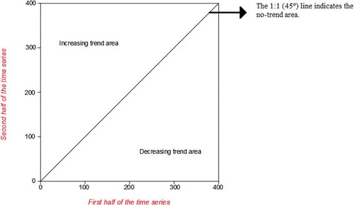
To avoid all the restrictive requirements (such as serial correlation, length, distribution of data) for application of the classical MK and SR trend methods, an innovative method has been developed by Sen (2012). Sen’s trend method (STM) is a modern, simple, easy to interpret, and effective trend analysis procedure that incorporates preliminary visual inspection for identification of the trend type whether increasing, decreasing or no trend cases (Sen 2017). Hence, this method has attracted increasing attention within hydrological studies in recent years (e.g. Sonali and Kumar 2013, Alipour et al. 2018). In this method, a time series is divided into two equal parts, with each part sorted in ascending order. Then, the first half series (x_i) is located on the x-axis, and the second half series (x_j) is located on the y-axis of a Cartesian coordinate system, producing a scatter plot, as shown in Figure 1. If data points on the diagram are on the 1:1 (45°) straight line, there is no trend in the time series (i.e. it is trendless). If data points are below the 1:1 line, it means that there is a decreasing trend, and if they are above the 1:1 line, it can be said that there is an increasing trend. Thanks to this method, possible changes (trends) in low, medium and high values of time series can be clearly seen.

Figure 1. Demonstration of increasing, decreasing and trendless areas according to Sen’s trend method on a Cartesian coordinate system.

3 Study area and data

Turkey is located between latitudes 36–42°N and longitudes 26–45°E. The country has four main climate types. In general, the climate is Mediterranean, which is generally seen in the Mediterranean and Aegean regions, with mild, wet winters (December, January and February) and warm to hot, dry summers (June, July and August). The Black Sea climate, which is mainly dominant in the coastal areas of Turkey bordering the Black Sea, is a temperate oceanic climate, with warm, wet summers and cool to cold, wet winters. Central, eastern, southeastern and west-central Anatolia experience typical land climate, with hot and dry summers and cold winters. Finally, the climate in the Marmara region is generally mild and humid in summer, and cold with above-average snow and rainfall in winter. The climate close to the shoreline in the Aegean region is typically Mediterranean, but inland it becomes cooler in winter, with a fairly high amount of snow at high altitudes (Haktanir and Citakoglu 2014, Guclu 2018).

The average annual rainfall of Turkey is 643 mm and yearly mean flow of the rivers is about 186 × 10⁹ m³ (Oktem and Aksoy 2014). Life is affected by disasters, such as earthquakes, floods, landslides and hurricanes. Floods, which cause the greatest loss of life and property after earthquakes, occur as a result of heavy rain and snowmelt. It is estimated that 28% of disasters in Turkey have occurred due to floods (Ersoy and Ozmen 2017). The Republic of Turkey’s Ministry of Forestry and Water Affairs General Directorate of Water Management (2017) recorded the details of 1209 flood events, which caused 720 deaths and damaged an area of 893–933 ha between 1975 and 2015. Hence, statistical evaluation of floods is crucial for the adequate design and operation of water resources systems and to ensure public safety. The existence of a significant trend in the annual maximum flows of rivers carries significance for different types of water resources problems (Cigizoglu et al. 2005).

In this study, the aim is to analyse possible significant changes in annual instantaneous maximum flows (AIMF) of Turkey’s rivers. The AIMF records of 153 flow stations operated by the DSI (General Directorate of State Hydraulic Works) are used for the applications. The main reason for choosing these stations is that the observations have not been influenced by human intervention, showing homogeneity and no missing values. The record lengths vary from 28 to 54 years, which can be considered as statistically valid. Burn and Elnur (2001) pointed out that the selection of gauge stations is a crucial step for climate change analysis and that stations having a minimum record length of 25 years ensures validity of the trend results statistically. The geographical distribution of the gauge stations under study is shown in Figure 2, and Table 1 presents basic information of the study basins.

Table 1. Turkish river basins with selected gauging stations and their basic statistical characteristics.

Basin no.	Basin name	Stations	Area of basin (× 10^3 km^2)	Basin average height (m)	Average precipitation (mm/year)	Total streamflow (km^3/year)
1	Meriç	101,103,106	14.560	56.63	604.0	1.33
2	Marmara	211,212,213,214,215	24.100	42.25	728.7	8.33
3	Susurluk	302,311,314,316,317,321,324,328	22.399	201.56	711.6	5.43
4	Aegean	410	10.003	63.75	624.2	2.09
5	Gediz	509,514,515,518,522,523,524,525,527	18.000	220.06	603.0	1.95
6	Little Menderes	601	6.907	4.00	727.4	1.19
7	Big Menderes	701,704,706,712,713,730,732,733,734	24.976	413.83	664.3	3.03
8	West Mediterranean	808,809,811,812,815,818	20.953	383.47	875.8	8.93
9	Central Mediterranean	902,912,917,918	19.577	248.85	100.4	11.06
10	Burdur Lake	-	6.374	910.0	446.3	0.50
11	Afyon	1102	7.605	1016.67	451.8	0.49
12	Sakarya	1203,1218,1219,1221,1222,1224,1226,1233,1237,1250	58.160	508.62	524.7	6.40
13	West Black Sea	1302,1307,1314,1319,1327,1330,1331,1332,1334,1335,1338,1339,1340	29.598	325.67	811.0	9.93
14	Yeşilırmak	1401,1402,1412,1413,1414,1418,1422,1424,1427	36.114	695.63	496.5	5.80
15	Kızılırmak	1501,1517,1532,1535,1538,1539,1541	78.180	748.48	446.1	6.48
16	Middle Anatolia	1611,1612,1621,1622	53.850	1139.37	416.8	4.52
17	East Mediterranean	1712,1714,1717,1719,1720,1721	22.048	269.05	745.0	11.07
18	Seyhan	1801,1805,1818,1820,1822	20.450	749.68	624.0	8.01
19	Hatay	1905,1906,1907,1908	7.796	159.17	815.6	1.17
20	Ceyhan	2004,2006,2008,2009,2020,2022,	21.982	684.81	731.6	7.18
21	Euphrates	2102,2115,2122,2124,2131,2133,2135,2145,2149,2151,2154,2156,2158,2164,2166,2177	127.304	1009.87	540.1	31.61
22	East Black Sea	2202,2213,2215,2218,2232,2233,2238,2245,2247	24.077	443.24	1198.2	14.90
23	Çoruh	2304,2305,2316,2320,2321,2323,2325,2328,2329,2330,	19.872	757.39	629.4	6.30
24	Aras	2409,2415,2418	27.548	1652.65	432.4	4.63
25	Van Lake	2505	19.405	1829.29	474.3	2.39
26	Tigris	2610,2612,2624	57.614	844.79	807.2	21.33
		Total	Total	Average	Average	Average
		153	779.452	591.49	658.86	186.05

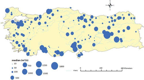
Skewness coefficients of the AIMF series were computed and found to be mostly positive, with skewness values in the range −0.42 to 5.76, where high skewness implies a right heavy-tailed distribution, and low skewness around zero a normal distribution. It is also observed that high skewness mostly occurred in the AIMF series of the stations located in western and southern rivers of Turkey. In the field of hydrology, all kinds of time series are generally positively skewed, and basic statistical characteristics including the mean and standard deviation may not provide sufficient information for the development and management of water resources in any region. This is because the mean and standard deviation may not able to describe the characteristics of the data values well when the data series are skewed. In addition, these basic characteristics are greatly affected by outliers. The median and other percentile values, which are robust basic statistics, are more useful when one is dealing with skewed hydrological data (Machiwal and Jha 2012). Hence, the median values of the AIMF series were computed and are presented in Figure 3. The median values vary between approx. 5 and 1840 m³/s, and tend to be rather higher at stations located along southern rivers of Turkey. The highest median value was observed at station 2112, which is located in the Euphrates basin (see Fig. 2). In addition, the coefficient of variation (CV) was adopted to reflect the degree of variation in dispersion of the AIMF series. The CV values of the stations located in the southern and western river basins are larger than those of the other river basins. The highest CV value of the AIMF series was found at station 1717, indicating that the AIMF at this station has the highest inter-annual variability.

Figure 2. Study area and spatial distribution of streamflow gauge stations used in the present study.

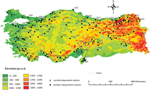
Figure 3. Map of median magnitudes of the AIMF series used in this study.

4 Results

4.1 Serial correlation analysis

Prior to applying the MK and SR tests to identify trends over the AIMF time series, serial autocorrelation structures of the data have to be checked. For this purpose, the lag-1 autocorrelations $\left(r_1\right)$ were computed and their statistical significance tested against the null hypothesis at a 95% confidence interval, using a two-tailed test, i.e. $r_1\left(95\mathrm{\%}\right)=\pm 1.96/\sqrt{N}.$

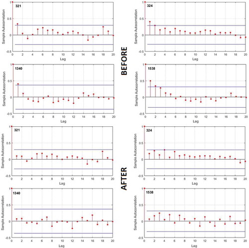
According to the results, the AIMF series of 24 stations showed a significant lag-1 autocorrelation (Table 2). The TFPW method was then used to remove these significant autocorrelations from the AIMF series and the new lag-1 autocorrelations, which were also included in Table 2, were computed. As can be seen from the table, the significant serial autocorrelations were successfully eliminated. For visual assessment, the correlograms of the AIMF series are also given in Figure 4. Here, only four examples of the stations are presented to control the length of the paper. It is obvious from Figure 4 that after applying the TFPW method the new autocorrelation coefficients (from 0 to 20 lags) are within the 95% confidence limits.

Table 2. The computed lag-1 autocorrelations, which are statistically significant, and the MK and SR test results (before and after the TFPW method).

Station no.	Before TFPW^a			Before TFPW^b		After TFPW^c			After TFPW^d		mMK		1.96/√N*
	lag-1	Z	Trend	Z	Trend	lag-1	Z	Trend	Z	Trend	Z	Trend
106	0.30	1.382	–	1.235	–	–0.01	1.572	–	1.279	–	0.934	–	0.28
311	0.34	–3.512	↓	–3.698	↓	–0.05	–3.022	↓	–3.119	↓	–3.512	↓	0.27
316	0.55	–5.437	↓	–5.195	↓	0.13	–4.885	↓	–4.626	↓	–6.037	↓	0.27
317	0.35	–2.383	↓	–2.622	↓	0.09	–2.912	↓	–3.073	↓	–2.383	↓	0.28
321	0.33	–3.230	↓	–3.248	↓	0.09	–2.897	↓	–2.928	↓	–3.027	↓	0.28
324	0.40	–3.662	↓	–3.648	↓	0.17	–3.724	↓	–3.635	↓	–3.662	↓	0.28
518	0.59	–5.789	↓	–5.478	↓	0.26	–5.370	↓	–5.016	↓	–5.788	↓	0.27
601	0.28	–3.093	↓	–2.959	↓	0.05	–2.959	↓	–2.983	↓	–3.093	↓	0.27
706	0.64	–4.387	↓	–4.099	↓	0.25	–5.580	↓	–5.163	↓	–4.546	↓	0.26
712	0.36	–5.014	↓	–5.075	↓	–0.05	–5.058	↓	–4.893	↓	–5.013	↓	0.26
713	0.42	–5.627	↓	–5.165	↓	0.15	–5.453	↓	–4.838	↓	–5.626	↓	0.27
818	0.43	2.728	↑	2.513	↑	0.12	2.935	↑	2.890	↑	3.377	↑	0.43
1340	0.40	–2.927	↓	–2.970	↓	0.07	–2.462	↓	–2.484	↓	–2.926	↓	0.35
1401	0.44	–4.241	↓	–4.270	↓	0.16	–4.233	↓	–4.268	↓	–4.241	↓	0.27
1402	0.38	–4.545	↓	–4.453	↓	0.13	–4.553	↓	–4.388	↓	–5.656	↓	0.27
1412	0.49	–4.600	↓	–4.440	↓	0.20	–4.758	↓	–4.629	↓	–2.554	↓	0.27
1501	0.27	–3.805	↓	–3.711	↓	0.05	–3.984	↓	–4.022	↓	–3.805	↓	0.26
1538	0.49	–2.937	↓	–2.928	↓	0.06	–2.855	↓	–3.001	↓	–2.332	↓	0.30
1719	−0.33	–0.967	–	–1.105	–	0.02	–0.338	–	–0.336	–	–0.967	–	0.30
1801	0.30	–0.259	–	–0.338	–	0.03	–0.301	–	–0.396	–	–0.259	–	0.27
1822	0.38	–3.915	↓	–3.917	↓	0.07	–3.934	↓	–4.019	↓	–3.914	↓	0.29
2004	0.32	–3.884	↓	–3.771	↓	0.08	–3.611	↓	–3.643	↓	–3.884	↓	0.29
2006	0.32	–1.201	–	–1.231	–	–0.01	–1.194	–	–1.269	–	–1.201	–	0.26
2020	0.57	–4.726	↓	–4.676	↓	0.17	–5.207	↓	–4.825	↓	–3.911	↓	0.28

*Critical value at the α = 0.05 significance level.

^aMK test results at 95% significance level (before applying TFPW).

^bSR test results at 95% significance level (before applying TFPW).

^cMK test results at 95% significance level (after applying TFPW).

^dSR test results at 95% significance level (after applying TFPW).

Figure 4. Autocorrelation plots (before and after pre-whitening) of the AIMF series for selected stations.

4.2 Results of the trend tests

4.2.1 MK and SR trend tests

Since the AIMF series generally have high positive skewness, which implies a right heavy tailed distribution, it is more suitable to consider non-parametric trend methods, such as the MK and SR tests described in Sections 2.2 and 2.3.

According to the MK test results, there is a statistically increasing trend in the AIMF series of six stations, while the data of 57 stations showed a significantly decreasing trend. No significant positive or negative trend was observed in the AIMF series for the remaining stations. The SR test yielded results that are mostly similar to those obtained by the MK test. Moreover, the SR test detected a decreasing trend for the AIMF series of stations 523 and 2325, although there was no significant trend for these stations according to the MK test. The results of both tests are presented in Figure 5.

Figure 5. Spatial representation of the MK and SR trend test results with a significance level of 0.05 for the AIMF series.

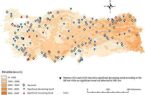
In addition to the simple MK test, the modified MK (mMK) test was implemented to analyse trends in the AIMF series having serial correlation. Also, the simple MK test was applied to these series after applying TFPW. It is well known that there are two options for evaluating trends in serial correlated data series. The first is to apply the modified trend test that can deal with significant autocorrelation structure in the data series, and the second is to apply a pre-whitening method to remove the existing serial correlation from the original data series. There is no consensus among researchers regarding which option provides a better trend evaluation. Hence, both options were used to evaluate trends in the serial correlated AIMF series in order to obtain the precise trend assessment. Both results are illustrated and compared in Table 2. It is clearly seen from Table 2 that the mMK test gave similar results to the simple MK (both before and after TFPW) and SR tests, although there was a slight difference between their Z scores.

4.2.2 Sen’s slope method

Sen’s slope method was applied to evaluate the magnitude of trends in the AIMF series; the results are given in Figure 6. As can be seen from Figure 6, the magnitude of the trends varies between −6.49 and 3.56 m³/s. The maximum significant decrease and increase were observed in the AIMF series of stations 1907 (6.49 m³/s) and 1621 (3.56 m³/s), respectively. The change percentage was also calculated over 153 stations using the formula given by Mondal et al. (2015);

(15) $\mathrm{P}\mathrm{e}\mathrm{r}\mathrm{c}\mathrm{e}\mathrm{n}\mathrm{t}\mathrm{a}\mathrm{g}\mathrm{e}\mathrm{c}\mathrm{h}\mathrm{a}\mathrm{n}\mathrm{g}\mathrm{e}\left(\mathrm{\%}\right)=\frac{Q\times N}{\bar{X}}\times 100$(15)

Figure 6. Spatial pattern of the trend magnitudes computed using Sen’s slope method.

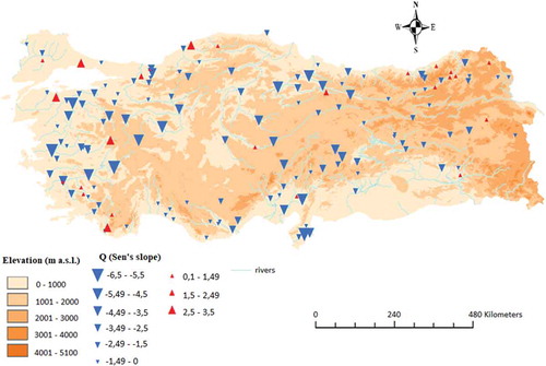
where N is the length of the AIMF series and $\bar{X}$ denotes the mean value of the AIMF series. The highest computed percentage change for significant negative trends was observed in the AIMF series of station 1102 (−24.64%; slope: −5.04 m³/s); and the highest percentage change for significant positive trends was observed in the AIMF series of station 524 (5.29%; slope: 2.93 m³/s).

4.2.3 Sen’s trend method (STM) results

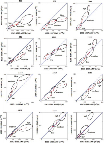
The STM was applied to each AIMF series explained in the previous section. Each data series was divided into three groups: low, medium and high, by considering the 50th and 90th percentiles (P) of the time series for definition of the bounds (< 50th P for the low cluster; > 50th and < 90th P for the medium cluster; and > 90th P for the high cluster). The results are given in Table 3; the trend evaluation of the low, medium and high values for each station was evaluated using Sen’s scatter diagram. To illustrate what was done for each station subjected to the diagrams, 12 gauge stations were randomly selected and their scatter diagrams are plotted in Figure 7. From Figure 7, it is clear that there is an increasing trend for all ranges of flows of station 1338, whereas medium and high flows of station 809 indicate increasing trends as the data points are generally located in the upper area of the 1:1 line. Comparatively high-flow (> 150 m³/s) trends show shorter duration than medium flows (> 60 and < 150 m³/s). There is a considerably increasing trend in high flows (> 270 m³/s) of stations 1222 and 2409, whereas no trend was observed for low and medium flows. According to the Sen graphs of stations 302 and 917, medium and high flows have decreasing trends and the low-flow clusters are trend free (trendless), the scatter of points being mainly located on the 1:1 line. The low, medium and high flows of stations 509 and 1535 have decreasing trends, implying that there is a decrease in all the clusters of the AIMF series in the second half of the historical records (1988–2012/1989–2014) with respect to the first half (1963–1987/1963–1988). Moreover, it is also obvious that the medium flows represent longer duration than the low and high flows. From the Sen graph of station 1414, it can be seen that all clusters of the AIMF series represent a decreasing trend, but the medium cluster has a slightly decreasing level. A decreasing trend is observed for medium (> 500 and < 1000 m³/s) and high (> 1000) flows of station 1805, while there is no trend for the low cluster. In the Sen graph of station 1219, a decreasing trend is observed for high flows (> 180 m³/s), while there is an increasing trend for low flows (< 120 m³/s). The AIMF series of station 2233 were found to be trendless, as the scatter points mostly take their positions on a curve.

Table 3. Performance evaluation and comparison of the MK and Sen’s trend methods for all the stations in this study.

Station no.	STM (m^3/s)			MK	Station no.	STM (m^3/s)			MK	Station no.	STM (m^3/s)			MK	Station no.	STM (m^3/s)			MK
	L	M	H			L	M	H			L	M	H			L	M	H
101	0–60 ▼	60–140 ▼	140–320 ▼	▼	515	0–160 –	160–470 ▼	470–1260 ▼	–	811	0–100 ▼	100–250 ▼	250–500 ▼	▼	1302	0–200 ▼	200–350 ▼	350–550 ▼	▼
103	0–700 –	700–1300 –	1300–1800 –	–	518	0–240 ▼	240–500 ▼	500–820 ▼	▼	812	0–600 ▼	600–1000 ▼	1000–1500 ▼	–	1307	0–100 –	100–180 ▲	180–230 ▲	–
106	0–150 ▲	150–400 ▼	400–660 ▼	–	522	0–160 ▼	160–420 ▼	420–900 ▼	▼	815	0–380 –	380–750 ▼	750–1350 ▼	–	1314	0–250 ▼	250–480 –	480–700 ▼	–
211	0–40 –	40–80 ▲	80–280 ▲	▲	523	0–200 –	200–500 ▼	500–1300 ▼	–	818	0–120 ▲	120–200 ▲	200–300 ▲	▲	1319	0–60 –	60–170 –	170–380 –	–
212	0–380 –	380–630 ▼	630–1800 ▼	–	524	0–20 ▲	20–40 ▲	40–100 –	▲	902	0–800 –	800–1450 –	1450–2600 ▼	–	1327	0–100 ▼	100–180 ▼	180–230 ▼	▼
213	0–40 –	40–80 –	80–120 –	–	525	0–20 –	20–40 ▼	40–160 ▼	▼	912	0–520 –	520–780 ▼	780–920 –	–	1330	0–10 –	10–20 –	20–140 –	–
214	0–110 –	110–310 –	310–440 ▼	–	527	0–200 –	200–500 –	500–1600 ▼	–	917	0–400 –	400–900 ▼	900–1250 ▼	–	1331	0–370 –	370–900 ▲	900–1450 ▲	▲
215	0–100 ▲	100–160 ▲	160–610 ▲	▲	601	0–100 ▼	100–280 ▼	280–700 ▼	▼	918	0–730 –	730–1250 ▼	1250–1650 ▼	–	1332	0–70 ▼	70–90 ▼	90–110 ▼	▼
302	0–500 –	500–1200 ▼	1200–2500 ▼	▼	701	0–230 ▼	230–390 ▼	390–560 ▼	▼	1102	0–5 ▼	5–15 ▼	15–50 ▼	▼	1334	0–60 –	60–90 –	90–270 –	–
311	0–50 ▼	50–150 ▼	150–200 ▼	▼	704	0–80 –	80–180 –	180–480 –	–	1203	0–30 ▼	30–90 ▼	90–220 ▼	▼	1335	0–900 ▼	900–1800 ▼	1800–2820 ▼	–
314	0–580 –	580–1390 ▼	1390–1700 –	–	706	0–180 ▼	180–300 ▼	300–410 ▼	▼	1218	0–300 ▼	300–450 –	450–610 ▼	–	1338	0–70 ▲	70–200 ▲	200–260 ▲	–
316	0–620 ▼	620–1240 ▼	1240–2400 ▼	▼	712	0–100 ▼	100–220 ▼	220–540 ▼	▼	1219	0–120 ▲	120–180 –	180–270 ▼	–	1339	0–40 –	40–90 –	90–170 –	–
317	0–470 ▼	470–770 ▼	770–970 ▼	▼	713	0–30 ▼	30–50 ▼	50–110 ▼	▼	1221	0–400 ▼	400–700 ▼	700–1010 ▼	▼	1340	0–240 –	240–450 ▼	450–900 ▲	▼
321	0–120 ▼	120–180 ▼	180–360 ▼	▼	730	0–10 –	10–70 ▲	70–190 ▼	–	1222	0–160 –	160–270 –	270–400 ▲	–	1401	0–400 ▼	400–680 ▼	680–1030 ▼	▼
324	0–240 ▼	240–380 ▼	380–550 ▼	▼	732	0–340 –	340–950 ▼	950–110 –	–	1224	0–20 ▼	20–40 ▼	40–90 ▼	▼	1402	0–600 ▼	600–950 ▼	950–1260 ▼	▼
328	0–70 –	70–180 ▼	180–280 ▼	▼	733	0–60 –	60–180 ▲	180–280 ▲	–	1226	0–60 ▼	60–160 ▼	160–210 ▼	▼	1412	0–40 ▼	40–120 ▼	120–180 ▼	▼
410	0–30 –	30–90 –	90–110 ▼	–	734	0–340 –	340–550 ▲	550–600 ▲	–	1233	0–180 ▼	180–420 ▼	420–680 ▼	–	1413	0–320 ▼	320–500 –	500–740 ▼	–
509	0–125 ▼	125–250 ▼	250–440 ▼	–	808	0–40 ▼	40–80 ▼	80–180 ▼	–	1237	0–50 –	50–150 ▼	150–260 ▼	–	1414	0–100 ▼	100–180 ▼	180–260 ▼	▼
514	0–100 ▼	100–500 ▼	500–1000 ▼	▼	809	0–60 –	60–150 ▲	150–260 ▲	–	1250	0–20 –	20–120 ▼	120–150 –	–	1418	0–180 –	180–250 –	250–500 –	–
1422	0–70 –	70–120 –	120–230 ▼	–	1801	0–200 –	200–400 –	400–710 ▼	–	2133	0–520 –	520–800 –	800–1340 –	–	2304	0–80 –	80–160 –	160–300 –	–
1424	0–30 –	30–60 –	60–90 –	–	1805	0–500 –	500–1000 ▼	1000–2000 ▼	–	2135	0–30 –	30–60 –	60–130 ▼	–	2305	0–360 –	360–570 ▲	570–700 –	–
1427	0–200 ▼	200–500 ▼	500–630 ▼	▼	1818	0–1000 –	1000–1950 –	1950–3280 ▼	–	2145	0–100 ▼	100–200 ▼	200–370 ▼	▼	2316	0–240 –	240–400 ▲	400–560 –	–
1501	0–360 ▼	360–680 ▼	680–1100 ▼	▼	1820	0–140 –	140–220 –	220–530 ▼	–	2149	0–320 ▲	320–480 –	480–1140 ▼	–	2320	0–160 –	160–260 –	260–330 –	–
1517	0–50 ▼	50–100 ▼	100–370 ▼	▼	1822	0–70 ▼	70–100 ▼	100–190 ▼	▼	2151	0–430 –	430–700 –	700–1020 –	–	2321	0–80 –	80–100 –	100–130 ▲	–
1532	0–420 –	420–800 –	800–1410 –	–	1905	0–100 –	100–180 –	180–270 –	–	2154	0–160 –	160–240 –	240–370 ▲	–	2323	0–230 –	230–360 –	360–510 –	–
1535	0–300 ▼	300–500 ▼	500–600 ▼	–	1906	0–170 ▼	170–380 ▼	380–1000 ▼	▼	2156	0–600 –	600–970 ▼	970–1160 –	–	2325	0–70 ▼	70–150 ▼	150–200 ▼	–
1538	0–120 ▼	120–210 ▼	210–560 ▼	▼	1907	0–110 ▼	110–180 ▼	180–200 ▼	▼	2158	0–210 –	210–38 ▼	380–760 ▼	▼	2328	0–40 ▼	40–70 ▼	70–90 ▼	▼
1539	0–160 ▼	160–300 ▼	300–370 ▼	▼	1908	0–370 ▼	370–590 –	590–1010 ▲	–	2164	0–500 –	500–800 ▼	800–1100 ▼	–	2329	0–160 –	160–300 ▲	300–400 ▲	–
1541	0–100 ▼	100–190 ▼	190–230 ▼	▼	2004	0–860 –	860–1340 ▼	1340–2500 ▼	▼	2166	0–600 –	600–1250 ▼	1250–1500 ▼	–	2330	0–20 ▼	20–30 ▼	30–60 ▼	▼
1611	0–30 –	30–60 –	60–180 –	–	2006	0–50 –	50–80 –	80–150 ▼	–	2177	0–240 ▼	240–350 ▼	350–530 ▼	▼	2409	0–120 –	120–270 –	270–610 ▲	–
1612	0–15 –	15–30 ▼	30–45 ▼	–	2008	0–140 –	140–250 –	250–600 –	–	2202	0–90 –	90–150 –	150–270 –	–	2415	0–160 –	160–280 –	280–400 ▲	–
1621	0–40 ▲	40–60 ▲	60–70 ▲	▲	2009	0–60 –	60–140 –	140–500 ▼	▼	2213	0–120 –	120–220 ▼	220–400 ▼	–	2418	0–140 –	140–320 –	320–770 –	–
1622	0–5 –	5–15 ▼	15–45 ▼	▼	2020	0–570 ▼	570–1650 ▼	1650–2000 ▼	▼	2215	0–80 –	80–110 –	110–190 –	–	2505	0–70 –	70–130 –	130–220 ▼	–
1712	0–220 –	220–380 –	380–520 ▼	–	2022	0–40 –	40–130 ▼	130–200 ▼	–	2218	0–140 –	140–280 ▼	280–510 ▼	▼	2610	0–200 –	200–370 –	370–450 –	–
1714	0–720 ▼	720–1250 ▼	1250–2000 –	▼	2102	0–1800 –	1800–3000 ▼	3000–3560 ▼	–	2232	0–150 –	150–250 –	250–560 ▼	–	2612	0–1330 ▼	1330–2000 ▼	2000–2670 ▼	▼
1717	0–20 –	20–60 –	60–440 –	▼	2115	0–380 –	380–700 ▼	700–2320 ▼	▼	2233	0–40 –	40–60 –	60–80 –	–	2624	0–240 –	240–440 –	440–600 –	–
1719	0–630 –	630–1100 –	1100–2500 ▲	–	2122	0–490 –	490–870 –	870–1130 –	–	2238	0–150 –	150–230 –	230–510 ▼	–
1720	0–280 –	280–550 –	550–700 ▼	–	2124	0–40 ▼	40–70 ▼	70–110 ▼	▼	2245	0–220 –	220–550 –	540–1000 –	–
1721	0–250 –	250–400 –	400–640 ▼	–	2131	0–15 –	15–50 ▼	50–160 ▼	▼	2247	0–350 ▼	350–1000 ▼	1000–1300 ▼	▼

▲,▼ and – symbols represent increasing trend, decreasing trend and no trend, respectively.

STM indicates Sen’s trend method.

L, M and H represent low, medium and high flows, respectively.

Figure 7. Results of Sen’s trend method for selected stations.

4.2.4 Comparison of the STM and the MK/SR test results

The results of the STM are compared with the traditional MK tests results and summarized in Table 3 (the SR results are not included as the test gave similar results to the MK test). It can be clearly seen from Table 3 that the STM generally yields similar trend results to the MK (and SR) test. However, the STM has the ability to detect trends for AIMF series of stations in which no trend was observed by the MK (SR) test. For station 1307, although there was no significant trend according to the MK (SR) test, the STM detected increasing trends in medium and high flows. Similar results were also observed for the medium and high flows of stations 733, 734, 809 and 2329. In other words, the medium and high flows have increases in the second half of the observation period compared with the first half. The STM showed a significantly increasing trend for all flow ranges of station 1338, in which no trend was detected by the MK (SR) test. These increasing trends give warning that floods are likely to increase in the future.

For the AIMF series of stations 106, 509, 808, 812, 1233, 1335, 1338, 1535 and 2325, the STM demonstrated decreasing or increasing trends for all ranges, while no significant trend was indicated by the MK (SR) test. Similarly, the MK (SR) test detected no significant trend in the AIMF series of stations 212, 515, 523, 815, 917, 918, 1237, 1612, 2022, 2102, 2164, 2166 and 2213, in which there are significant decreasing trends in the medium and high flows according to the STM.

5 Discussion

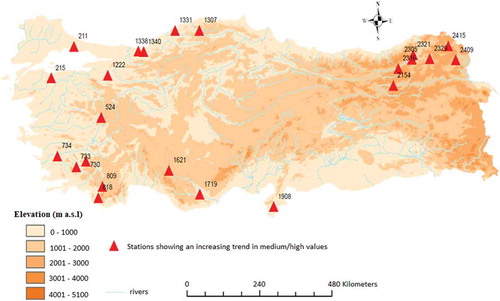
According to the MK, mMK and SR trend tests that were applied to AIMF records of 153 flow stations having record lengths greater than or equal to 28 years, 57 stations showed a significant decreasing trend. However, the data of only six stations showed a significant increasing trend at the α = 0.05 significance level. It can be concluded that the detected negative trends are seen across the whole of Turkey, while positive trends are seen only in western Turkey. The findings of the MK, mMK and SR tests conducted in this study are generally parallel to those of the study by Cigizoglu et al. (2005), who evaluated trends in annual maximum flows of 96 gauge stations. They found trends at only 15 flow stations; among these significant trends, only four stations showed an increasing trend, while the remaining stations’ trends were decreasing. Moreover, Topaloglu (2006) evaluated trends in annual instantaneous maximum streamflow obtained from 84 gauge stations for a 30-year period (1968–1997). According to the MK test, the majority of the stations (66) showed negative trends, but only 26 stations, located mostly in the western part of Turkey, were found to be significant at the 5% level, while only two stations (located in the Coruh and Van Lake basins) exhibited statistically significant positive trends. In our study, a much wider view was taken, with a dense network of gauging stations and deep analysis of temporal changes in the annual instantaneous maximum streamflow of Turkish rivers. In this study, a new trend method was also employed to find significant changes in low, medium and high flows separately. Based on this innovative method, trends in medium and high flow values, which can cause more damage, can easily be detected. Figure 8 presents the spatial distribution of the detected increasing trends in medium or high flows. From Figure 8, it can be seen that 22 stations have significant increasing trends in medium and high clusters, which means that there is an increase in these flow ranges during the second half of the historic record with respect to the first half. However, only five (211, 215, 524, 1331 and 1621) of these stations displayed an increasing trend based on the MK or SR tests. The findings of the new method indicate that the risk of flood hazard in the northern, eastern and western rivers of Turkey is of serious concern. The Coruh basin, which is located in northeastern Turkey, has recently gained growing interest for the national economy, and regular joint technical meetings have been held between Turkish and Georgian experts concerning the construction of dams (Tosunoglu 2018). According to the Coruh Basin Development Plan, 27 dams and hydro-electric power plants are to be built along all rivers of the basin. The possible changes in AIMF series are significant, in particular for planning, design and management of these structures. Besides the potential benefits of the new trend method, the main disadvantage of this method is that it must be used for each data series individually, and the decision is made by expert visual observation, as it is a graphical method.

Figure 8. Spatial distribution of the increasing trends in medium or high clusters.

6 Conclusion

This study provides a comprehensive evaluation of long-term changes in annual instantaneous maximum flow (AIMF) records from 153 gauge stations uniformly distributed across 26 river basins of Turkey. Two traditional non-parametric trend tests – Mann-Kendall and Spearman’s rho (MK and SR) – and a new trend method – Sen’s trend method – were implemented for statistical evaluation of the trends. Moreover, Sen’s slope method was used to determine the magnitude of the trends. The results may be summarized as follows:

1. Lag-1 serial correlation was used to evaluate the presence of any existing correlation in the data series before applying the MK and SR tests, an approach that is often ignored in many trend detection studies. Using the trend-free pre-whitening (TFPW) method, the influence of serial correlation was successively eliminated from the time series of 24 stations.

2. The results of the MK, modified MK (which was also employed for the data of the stations having serial correlation) and SR tests reveal that the AIMF records of 57 stations experienced statistically decreasing trends in their flows, while six stations showed increasing trends.

3. Based on the results of Sen’s slope method, the magnitude of negative trend varies from −6.50 m³/s per year for station 1907, located in the Hatay River basin, to 0.01 m³/s per year for station 2149, in the Euphrates River basin, one of the most important sources of water for Turkey. In contrast, the magnitude of positive trend varies from 0.01 m³/s per year for station 2320, in the Coruh River basin, to 3.57 m³/s per year for station 1621 in the Middle Anatolia River basin.

4. Trend behaviours were investigated in more detail by Sen’s trend method, as the AIMF series were divided into three clusters (low, medium and high). Although this innovative method yielded similar results to the MK and SR tests, it discovered much more positive and negative trends, which could be a sign of flood risk to both human lives and the natural environment.

Acknowledgements

The authors acknowledge the General Directorate of State Hydraulic Works, Turkey, for providing the annual instantaneous maximum flow records used in this study. The authors also thank Mr Eren Ozbek, English Language Instructor at the Office of International Affairs, Erzurum Technical University, for improving the language of the manuscript.

Disclosure statement

No potential conflict of interest was reported by the authors.

Additional information

Funding

This study was supported by Erzurum Technical University Scientific Research Coordination Unit (Project No. 2017/10).

References

- Abeysingha, N.S., et al., 2016. Analysis of trends in streamflow and its linkages with rainfall and anthropogenic factors in Gomti River basin of North India. Theoretical and Applied Climatology, 123 (3–4), 785–799. doi:10.1007/s00704-015-1390-5
- Abghari, H., Tabari, H., and Talaee, P.H., 2013. River flow trends in the west of Iran during the past 40 years: impact of precipitation variability. Global and Planetary Change, 101, 52–60. doi:10.1016/j.gloplacha.2012.12.003
- Ahn, K.H. and Palmer, R.N., 2016. Trend and variability in observed hydrological extremes in the United States. Journal of Hydrologic Engineering, 21 (2), 04015061. doi:10.1061/(ASCE)HE.1943-5584.0001286
- Alipour, A., et al., 2018. Spatio-temporal analysis of groundwater level in an arid area. International Journal of Water, 12 (1), 66–81. doi:10.1504/IJW.2018.090185
- Bai, P., et al., 2016. Investigation of changes in the annual maximum flood in the Yellow River basin, China. Quaternary International, 392, 168–177. doi:10.1016/j.quaint.2015.04.053
- Bormann, H., Pinter, N., and Elfert, S., 2011. Hydrological signatures of flood trends on German rivers: flood frequencies, flood heights and specific stages. Journal of Hydrology, 404 (1–2), 50–66. doi:10.1016/j.jhydrol.2011.04.019
- Burn, D.H. and Elnur, M.A.H., 2001. Detection of hydrologic trends and variability. Journal of Hydrology, 255 (2002), 107–122. doi:10.1016/S0022-1694(01)00514-5
- Burn, D.H., Sharif, M., and Zhang, K., 2010. Detection of trends in hydrological extremes for Canadian watersheds. Hydrological Processes, 24 (13), 1781–1790. doi:10.1002/hyp.v24:13
- Burn, D.H. and Whitfield, P.H., 2016. Changes in floods and flood regimes in Canada. Canadian Water Resources Journal, 41 (1–2), 139–150. doi:10.1080/07011784.2015.1026844
- Ceribasi, G. and Dogan, E., 2015. The evaluation of the flow quantity of the Sakarya basin with the west and eastern black sea by using trend analysis metho. SDU International Technologic Science, 7 (2), 1–12.
- Cigizoglu, H.K., Bayazit, M., and Onoz, B., 2005. Trends in the maximum, mean, and low flows of Turkish rivers. Journal of Hydrometeorology, 6 (3), 280–290. doi:10.1175/JHM412.1
- Coch, A. and Mediero, L., 2016. Trends in low flows in Spain in the period 1949–2009. Hydrological Sciences Journal, Journal Des Sciences Haydrologiques, 61 (3), 568–584. doi:10.1080/02626667.2015.1081202
- Cunderlik, J.M. and Ouarda, T.B.M.J., 2009. Trends in the timing and magnitude of floods in Canada. Journal of Hydrology, 375 (3–4), 471–480. doi:10.1016/j.jhydrol.2009.06.050
- Dabanli, I., et al., 2016. Trend assessment by the innovative-sen method. Water Resources Management, 30 (14), 5193–5203. doi:10.1007/s11269-016-1478-4
- Dam, J.C.V., 1999. Impacts of climate change and climate variability on hydrological regimes. Cambridge, UK: University of Cambridge.
- Dixon, H., Lawler, D.M., and Shamseldin, A.Y., 2006. Streamflow trends in western Britain. Geophysical Research Letters, 33 (19). doi:10.1029/2006GL027325
- Douglas, E.M., Vogel, R.M., and Kroll, C.N., 2000. Trends in floods and low flows in the United States: impact of spatial correlation. Journal of Hydrology, 240 (1–2), 90–105. doi:10.1016/S0022-1694(00)00336-X
- Ersoy, S. and Ozmen, B., 2017. Statistical evaluation of natural disaster losses occuring world and Turkey in 2006 year. Turkey (in Turkish).
- Guclu, Y.S., 2018. Multiple Şen-innovative trend analyses and partial Mann-Kendall test. Journal of Hydrology, 566, 685–704. doi:10.1016/j.jhydrol.2018.09.034
- Gumus, V. and Yenigun, K., 2006. Evaluation flows of lower Euphrates basin by trend analysis. In: Seventh international congress on advances in civil engineering. Istanbul, Turkey: Yildiz Technical University, 1–12.
- Haktanir, T. and Citakoglu, H., 2014. Trend, independence, stationarity, and homogeneity tests on maximum rainfall series of standard durations recorded in Turkey. Journal of Hydrologic Engineering, 19 (9), 05014009. doi:10.1061/(ASCE)HE.1943-5584.0000973
- Hamed, K.H. and Rao, A.R., 1998. A modified Mann-Kendall trend test for autocorrelated data. Journal of Hydrology, 204 (1–4), 182–196. doi:10.1016/S0022-1694(97)00125-X
- Hu, Y.R., et al., 2011. Streamflow trends and climate linkages in the source region of the Yellow River, China. Hydrological Processes, 25 (22), 3399–3411. doi:10.1002/hyp.8069
- Kahya, E. and Kalayci, S., 2004. Trend analysis of streamflow in Turkey. Journal of Hydrology, 289 (1–4), 128–144. doi:10.1016/j.jhydrol.2003.11.006
- Kendall, M.G., 1975. Rank correlation methods. London: Charless Griffin.
- Lins, H.F. and Slack, J.R., 2005. Seasonal and regional characteristics of US streamflow trends in the United States from 1940 to 1999. Physical Geography, 26 (6), 489–501. doi:10.2747/0272-3646.26.6.489
- Lopez-Moreno, J.I., Begueria, S., and Garcia-Ruiz, J.M., 2006. Trends in high flows in the central Spanish Pyrenees: response to climatic factors or to land-use change? Hydrological Sciences Journal-Journal Des Sciences Hydrologiques, 51 (6), 1039–1050. doi:10.1623/hysj.51.6.1039
- Machiwal, D. and Jha, M.K., 2012. Hydrologic time series analysis: theoryand practice. New Delhi, India: Capital Publishing Company.
- Mann, H.B., 1945. NONPARAMETRIC TESTS AGAINST TREND. Econometrica, 13 (3), 245–259. doi:10.2307/1907187
- Masih, I., et al., 2011. Streamflow trends and climate linkages in the Zagros Mountains, Iran. Climatic Change, 104 (2), 317–338. doi:10.1007/s10584-009-9793-x
- Mediero, L., et al., 2014. Detection and attribution of trends in magnitude, frequency and timing of floods in Spain. Journal of Hydrology, 517, 1072–1088. doi:10.1016/j.jhydrol.2014.06.040
- Mondal, A., Khare, D., and Kundu, S., 2015. Spatial and temporal analysis of rainfall and temperature trend of India. Theoretical and Applied Climatology, 122 (1–2), 143–158. doi:10.1007/s00704-014-1283-z
- Nune, R., et al., 2014. Relating trends in streamflow to anthropogenic influences: a case study of Himayat Sagar Catchment, India. Water Resources Management, 28 (6), 1579–1595. doi:10.1007/s11269-014-0567-5
- Oktem, U.A. and Aksoy, A., 2014. Water risk report of Turkey. Istanbul: WWF-Turkey (in Turkish).
- Panda, D.K., et al., 2013. Streamflow trends in the Mahanadi River basin (India): linkages to tropical climate variability. Journal of Hydrology, 495, 135–149. doi:10.1016/j.jhydrol.2013.04.054
- Petrow, T. and Merz, B., 2009. Trends in flood magnitude, frequency and seasonality in Germany in the period 1951–2002. Journal of Hydrology, 371 (1–4), 129–141. doi:10.1016/j.jhydrol.2009.03.024
- Radziejewski, M., 2011. About trend detection in river floods. In: J.P. Kropp and H.J. Schellnhuber, eds. In extremis disruptive events and trends in climate and hydrology. New York: Springer Heidelberg Dordrecht London, 145–165.
- Rao, A.R., Hamed, K., and Chen, H., 2003. Nonstationarities in hydrologic and environmental time series. Dordrecht, Netherlands: Kluwer Academic Publishers.
- Rice, J.S., et al., 2015. Continental US streamflow trends from 1940 to 2009 and their relationships with watershed spatial characteristics. Water Resources Research, 51 (8), 6262–6275. doi:10.1002/2014WR016367
- Sen, P.K., 1968. Estimates of the regression coefficient based on Kendall‘s Tau. Journal of the American Statistical Association, 63 (324), 1379–1389. doi:10.1080/01621459.1968.10480934
- Şen, Z., 2012. Innovative trend analysis methodology. Journal of Hydrologic Engineering, 17 (9), 1042–1046. doi:10.1061/(ASCE)HE.1943-5584.0000556
- Şen, Z., 2017. Innovative trend methodologies in science and engineering. Cham: Springer.
- Sonali, P. and Kumar, D.N., 2013. Review of trend detection methods and their application to detect temperature changes in India. Journal of Hydrology, 476, 212–227. doi:10.1016/j.jhydrol.2012.10.034
- Song, W.Z., et al., 2015. Annual runoff and flood regime trend analysis and the relation with reservoirs in the Sanchahe River Basin, China. Quaternary International, 380, 197–206. doi:10.1016/j.quaint.2015.01.049
- Tabari, H., et al., 2017. Decadal analysis of river flow extremes using quantile-based approaches. Water Resources Management, 31, 3371–3387. doi:10.1007/s11269-017-1673-y
- Tabari, H., Nikbakht, J., and Talaee, P.H., 2012. Identification of trend in reference evapotranspiration series with serial dependence in Iran. Water Resources Management, 26 (8), 2219–2232. doi:10.1007/s11269-012-0011-7
- Timbadiya, P.V., et al., 2013. Identification of trend and probability distribution for time series of annual peak flow in Tapi Basin, India. ISH Journal of Hydraulic Engineering, 19 (1), 11–20. doi:10.1080/09715010.2012.739354
- Topaloglu, F., 2006. Trend detection of streamflow variables in Turkey. Fresenius Environmental Bulletin, 15 (7), 644–653.
- Tosunoglu, F., 2017. Trend analysis of daily maximum rainfall series in Çoruh Basin,Turkey. Journal of the Institute of Science and Technology, 7 (1), 195–205. doi:10.21597/jist.2017127432
- Tosunoglu, F., 2018. Trend analyses of Turkish Euphrates Basin streamflow by innovative Sen‘s trend method and traditional Mann-Kendall test. Fresenius Environmental Bulletin, 27 (1), 446–458.
- Wang, H.J., Chen, Y.N., and Li, W.H., 2015. Characteristics in streamflow and extremes in the Tarim River, China: trends, distribution and climate linkage. International Journal of Climatology, 35 (5), 761–776. doi:10.1002/joc.2015.35.issue-5
- Yu, Y.S., Zou, S.M., and Whittemore, D., 1993. Nonparametric trend analysis of water-quality data of rivers in Kansas. Journal of Hydrology, 150 (1), 61–80. doi:10.1016/0022-1694(93)90156-4
- Yue, S., et al., 2002. The influence of autocorrelation on the ability to detect trend in hydrological series. Hydrological Processes, 16 (9), 1807–1829. doi:10.1002/hyp.1095
- Zamani, R., et al., 2017. Streamflow trend analysis by considering autocorrelation structure, long-term persistence, and Hurst coefficient in a semi-arid region of Iran. Theoretical and Applied Climatology, 129 (1–2), 33–45. doi:10.1007/s00704-016-1747-4
- Zang, C.F. and Liu, J.G., 2013. Trend analysis for the flows of green and blue water in the Heihe River basin, northwestern China. Journal of Hydrology, 502, 27–36. doi:10.1016/j.jhydrol.2013.08.022
- Zhang, Q., et al., 2006. Observed trends of annual maximum water level and streamflow during past 130 years in the Yangtze River basin, China. Journal of Hydrology, 324 (1–4), 255–265. doi:10.1016/j.jhydrol.2005.09.023
- Zhao, G.J., et al., 2010. Streamflow trends and climate variability impacts in Poyang Lake Basin, China. Water Resources Management, 24 (4), 689–706. doi:10.1007/s11269-009-9465-7