El Niño and La Niña influence on mean river flows of southern South America in the 20th century

ABSTRACT

The influence of the El Niño Southern Oscillation (ENSO) phenomenon on monthly mean river flows of 12 rivers in the extreme south of South America in the 20th century is analysed. The original dataset of each river is divided into two subsets, i.e. warm ENSO events or El Niño, and cold ENSO events or La Niña. The elements of the subsets are composites of 24 consecutive months, from January of the year when the ENSO event begins to December of the following year. The ENSO signal is analysed by comparing the monthly mean value of each subset to the long-term monthly mean. The results reveal that, in general, monthly mean El Niño (La Niña) river flows are predominantly larger (smaller) than the long-term monthly mean in the rivers studied. The anomalies are more evident during the second half of the year in which the event starts and the first months of the following year.

KEYWORDS:

• El Niño
• La Niña
• monthly mean river flow
• anomalies
• 20th century
• southern South America

Editor R. Woods Associate editor T. Kjeldsen

1 Introduction

The sea-surface temperature (SST) of the global oceans is a fundamental component of the climate system. The most active and prominent energy exchange between the surface of the Earth and the atmosphere is at the ocean–atmosphere interface. The short-term variations, from days to a few weeks, of the physical properties at the ocean surface are negligible in comparison to those over the continents. The tropical and subtropical oceans are a main source of energy and moisture for the atmosphere, so the slow SST changes become a key factor in modulating low-frequency climate variations worldwide. The best example of this is the El Niño Southern Oscillation (ENSO) phenomenon that develops in the equatorial and tropical regions of the Pacific Ocean. ENSO is known to be a major source of seasonal to inter-annual climate variability over several regions of the planet, many of which are remotely located. At the local scale, climate variability signals become more evident when averaging the observations in time and space, and the monthly mean river flows are a good example of that. The river flows summarize the hydrological balance of the entire basin so that their variations become, to a major degree, independent of the moment and location in which the individual weather events take place.

Different authors have studied the relationship between the SST variability over the equatorial and tropical oceans and seasonal to inter-annual variability of rainfall at both global and local scales (e.g. Ropelewski and Halpert 1987, Kiladis and Diaz 1989). For example, Dettinger et al. (2000) investigated the effects of El Niño/La Niña events on river flows throughout the American continent. They found persistent correlations between the peak-flow season river flows in North and South America and seasonal values of the Southern Oscillation Index (SOI). Amarasekera et al. (1997) examined the relationships between the annual discharges of the Amazon, Congo, Paraná and Nile rivers and the SST anomalies over the eastern and central equatorial Pacific Ocean. The results of that study show that the annual discharges of the Amazon and Congo rivers are weakly and negatively correlated with the equatorial Pacific SST anomalies, with 10% of the variance in annual discharges explained by ENSO. The Nile and Paraná rivers show stronger correlations, being positive for the Paraná and negative for the Nile. Similar studies linking ENSO with anomalous behaviour in rainfall or river flows have been carried out throughout the globe, such as McKerchar et al. (1998) and Mosley (2000) in New Zealand; Chiew et al. (1998) in Australia; Rimbu et al. (2004) in the Danube River, and Mohsenipour et al. (2013) in Iran. These studies show significant responses of those variables to the ENSO forcing which are consistent with the climatic effects already identified with the Southern Oscillation.

Several studies relate climate anomalies with the occurrence of ENSO events over South America as well. Berri and Flamenco (1998) found a positive correlation between the seasonal volume in October–March of the Diamante River (central Andes Mountains of Argentina) and SST anomalies over the Niño3 region of the Pacific Ocean during the previous March–April and simultaneous November–December. Berri et al. (2002) studied the influence of ENSO on the monthly flows of the Upper Paraná River. Their results show that the averaged flows observed during El Niño events are always larger than those observed during La Niña events. The difference between El Niño and La Niña river flows, with respect to the long-term average, peaks in November–December of the year when the ENSO events start. Pasquini and Depetris (2007) studied river flow variability in South America and reported El Niño-like inter-annual periodicities in most rivers of the region, including some in the southern cone of the continent. Araneo and Compagnucci (2008) determined statistical relationships between the SSTs over the Niño3 + 4 region of the Pacific Ocean and the flows of river systems of the central Andes Mountains in Argentina of up to 14 months in advance. The authors found that the correlation maps for river flows–SST revealed typical ENSO patterns over the Pacific Ocean. A recent study by Rivera et al. (2017) found a consistent El Niño signal accounting for wet conditions in the northern part of the southern cone of South America. However, there are no comprehensive studies focused on the ENSO influence on monthly mean flows of the most important rivers in the extreme south of South America.

The objective of this paper is to describe the influence of the ENSO phenomenon throughout the 20th century on the monthly mean flows, and at a seasonal time scale, of 12 rivers of southern South America, employing the longest time series available. Most of this region is semi-arid (the Atlantic watershed to the east of the Andes Mountains), so this set of rivers constitutes a significant source of potable water, as well as water for irrigation and hydropower generation. The Patagonian region where the studied watersheds are located is characterized by low population density and non-extensive exploitation of natural resources, so there are no reports of appreciable changes in the river flows that could have been caused by human activities. The Colorado River may be the only exception, because there is a dam upstream of the gauge station (this is discussed in Section 2). Therefore, any long-term change in river flows may be attributed to climate variability. It is certainly beyond the scope of this study to discuss the complex hydrology of this region in which rainfall, snowmelt and glacier melt contribute to river flows in different ways, so it is limited to describing and comparing the observed river flow departures from the long-term mean when ENSO occurs. It is also not the purpose of this study to discuss the physical mechanisms responsible for the inter-annual climate variability in this region; instead, we refer the reader to, for example, Garreaud et al. (2013) and references therein for more details. Section 2 describes the study area, the main characteristics of the different rivers and the data employed; Section 3 presents the methodology applied to study the ENSO influence on the mean river flows; Section 4 describes the results obtained for each river system; and Section 5 discusses the results. Finally, Section 6 presents the conclusions of the study.

2 Study area, hydrological regime and data

Figure 1 shows the locations of the 12 studied rivers in the southern extreme of South America, with the geographical distribution and size of the river basins and their long-term monthly mean river flows (m³ s⁻¹). Table 1 presents a list of the rivers, with an indication of the river flow gauge station data used in the study, the upstream drainage area (km²), long-term maximum and minimum monthly mean discharge (m³ s⁻¹), period of analysis, and the source of the data. The period of analysis varies between 25 and 100 years, depending on the data availability of each river. The time series of monthly mean river flows are from the Secretary of Hydric Resources of Argentina (www.hidricosargentina.gov.ar) and the General Water Directorate of Chile (www.dga.cl).

Table 1. River flow gauge stations used, listed from north to south, with upstream drainage area (km²), long-term maximum and minimum monthly mean discharge (m³ s⁻¹), period of analysis and data source. SHR: Secretary of Hydric Resources of Argentina; GWD: General Water Directorate of Chile.

River	Gauge station	Drainage (km^2)	Monthly discharge (m^3 s^−1)		Period of analysis	Data source
			Max	Min
Colorado	Pichi Mahuida	22 300	274	73	1919–2003	SHR
Neuquén	Paso de Indios	30 843	608	93	1904–2003	SHR
Limay	Paso Limay	26 400	1031	258	1904–1989	SHR
Cautin	Rari Ruca	1365	175	42	1930–2006	GWD
Tolten	Villarica	2880	440	131	1930–2006	GWD
Pilmaiquén	San Pablo	2680	298	84	1930–2006	GWD
Manso	Los Alerces	750	61	20	1952–2003	SHR
Futaleufú	Balsa Garzón	4608	351	164	1949–2001	SHR
Chubut	Los Altares	16 400	86	10	1944–2003	SHR
Santa Cruz	Charles Fuhr	15 550	1273	281	1957–2002	SHR
Grande	Tierra del Fuego	2725	48	11	1982–2006	SHR
San Juan	Desembocadura	860	32	7	1981–2006	GWD

Figure 1. Geographical distribution of the river basins in the southern extreme of South America, and long-term monthly mean river flows (m³ s⁻¹).

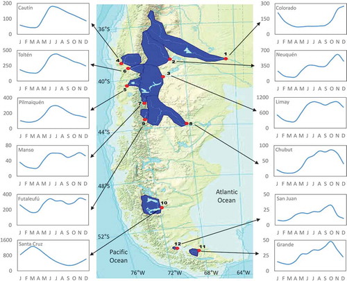
The distinctive feature of the regional geography is the meridionally oriented Andes mountain range on the western side of the continent. The average height in the northern part of the study region is 4000 m a.s.l. (with peaks over 5000 m), decreasing to about 2500 m a.s.l. towards the southern tip of the continent, with a northwest–southeast orientation. To the east of the Andes, the terrain heights decrease smoothly towards the Atlantic Ocean.

The high Andes Mountains are a barrier for the atmospheric flow that captures the moisture carried by the strong mid-latitude Westerlies, so that most precipitation falls on the windward side of the Andes and the mountain tops. The western slopes of the Andes receive precipitation all year round, with annual amounts of several thousand millimetres. In the northern part of the study region, the maximum precipitation is in winter, while towards the southern tip of the continent the maximum is in summer. However, a dramatic reduction of precipitation amounts takes places a few tens of kilometres eastward of the Andes, leaving semi-arid lands towards the Atlantic Ocean, where the annual precipitation is in the order of a few hundred millimetres (Garreaud et al. 2013).

The high mountain ranges receive precipitation in the form of snow, while the middle and lower ranges receive a combination of snow and rain. The steep terrain allows the rapid downslope flow of rainwater and the river flow response to rainfall is almost immediate, while the snow remains in place until the spring when snowmelt starts. The response of monthly mean river flows to the precipitation regime depends on what fraction of the river basin is in the higher, middle or lower mountain ranges. Another physical characteristic of the river basins that regulates river flows is the presence of upstream lakes, as well as glaciers that contribute to high river flows in the warm season, regardless of the amount of snow accumulated during the previous winter. It is not the purpose of this study to discuss the complex hydrology of the region, so we simply provide a brief description of the annual cycle of the long-term monthly mean river flows.

Five of the nine rivers in the northern part of the region have small basins of less than 5000 km² (see Table 1) and drain to the Pacific Ocean. Three of them – the Cautín, Toltén and Pilmaiquén rivers – display an annual river flow cycle with the maximum in July and the minimum in March (Fig. 1, left). The other two – the Manso and Futaleufú rivers – also have the winter maximum in June/July and the end of summer minimum in March, along with a secondary spring maximum in November due to the snowmelt.

The other four rivers in the northern part of the region – the Colorado, Neuquén, Limay and Chubut rivers – have large basins of more than 16 000 km² (Table 1) and discharge into the Atlantic Ocean. These rivers display a significant snowmelt component (Fig. 1, right), for example, the Neuquén and Limay rivers in November, the Chubut River in October and the Colorado River in December. With the exception of the Colorado River, they also present a secondary winter maximum, more significant in the case of the Limay River. The Colorado River displays a particular annual behaviour, with a prolonged minimum from March to September, which is a consequence of the combination of winter snowfalls and rain throughout the year. There is a large hydropower dam located 300 km upstream of the gauge station which regulates the river flows, although with minimum influence on the long-term mean since it affects only the last 7 years of the period of analysis.

In the southern part of the region, the Santa Cruz River (large basin of 15 550 km²) displays a typical glacier regime, with the maximum in March (the end of summer) and the minimum in September/October just before the melting starts. The smooth annual river flow cycle is a consequence of the regulating effect of two large lakes upstream of the gauge station. The Grande and San Juan rivers (small basins of 2725 and 860 km², respectively) present maximum river flows in October and minimum river flows in February/March, highlighting the relevant snowmelt contribution to the annual cycle.

3 Methodology

The ENSO events are characterized by a slow time evolution of SST anomalies over the equatorial and tropical Pacific Ocean. The ENSO-related SST anomalies generally begin during the first half of a calendar year, reach their peak by the end of the year, and thereafter they start to disappear (Trenberth 1997). Therefore, a complete ENSO event cycle includes two consecutive years and its consequences are felt to a variable degree by the affected regions at different moments of the event cycle. This behaviour can be seen in Figure 2, which shows the mean value of the Oceanic Niño Index (ONI) of El Niño and La Niña events, from 1950 when the index starts until 2006, the last year of the river flows database. The time evolution is presented as a 24-month period running from January of the year when the ENSO events starts (o) until December of the following year (+). The ONI is defined as the 3-month running mean of SST anomalies in the Niño3.4 region (5°N–5°S, 120°W–170°W). It is generally accepted to characterize ENSO events as warm or El Niño (cold or La Niña) when the ONI exceeds the +0.5°C (–0.5°C) threshold for a minimum of five consecutive overlapping seasons.¹ Although the ONI is not the only measure of ENSO, since other atmospheric and oceanic variables as well as combinations of them are also used, there is a consensus in the scientific community that other indices confirm features consistent with the phenomenon during these periods (Trenberth and Stepaniak 2001).

Figure 2. Oceanic Niño Index (ONI) average of El Niño (red) and La Niña (blue) events for the period 1950–2003. Values are 3-month running means of SST anomalies (°C) in the Niño3.4 region (5°N–5°S, 120°W–170°W), from February of the year when the ENSO event starts (o) until November of the following year (+).

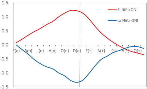
This study adopts a simple methodology that is appropriate for determining the influence of ENSO events on river flows at seasonal time scales. Two data subsets are created from the original time series of monthly river flows, one with the years of warm ENSO events (or El Niño), and the second with the years of cold ENSO events (or La Niña). The elements of the subsets are composites of 24 consecutive months starting in January of the year when an ENSO event starts (o) and ending in December of the following year (+). Berri et al. (2002) discuss the importance of considering the 2-year period since the equatorial Pacific Ocean SST anomalies peak at the end of the year when the ENSO event starts (see Fig. 2). Table 2 presents the list of ENSO events since 1902 used in the study, considering the most accepted classifications. From 1950 we adopt the criteria based on the ONI, i.e. a minimum of five consecutive overlapping seasons of 3-month running mean Niño3.4 SST anomalies exceeding the threshold of +0.5°C for warm events (El Niño) and −0.5°C for cold events (La Niña).

Table 2. List of warm (El Niño) and cold (La Niña) ENSO events considered in the study.

Warm ENSO (El Niño) events	Cold ENSO (La Niña) events
1902/03, 1905/06, 1911/12	1904/05, 1908/09
1914/15, 1918/19, 1923/24	1910/11, 1916/17
1925/26, 1930/31, 1932/33	1924/25, 1928/29
1939/40, 1941/42, 1951/52, 1953/54, 1957/58, 1958/59	1938/39, 1954/55 1955/56, 1964/65
1963/64, 1965/66, 1968/69	1970/71, 1971/72
1969/70, 1972/73, 1976/77	1973/74, 1974/75
1977/78, 1979/80, 1982/83 1986/87, 1987/88, 1991/92 1992/93, 1994/95, 1997/98 2002/03, 2004/05	1975/76, 1983/84 1984/85, 1988/89 1995/96, 1998/99 1999/00, 2000/01

Prior to 1950, when the ONI is not available, we adopt other widely acknowledged ENSO classifications. In the case of El Niño events, we use that of Rasmusson and Carpenter (1983), hereinafter RC, which is based on SST anomalies in the equatorial and tropical Pacific Ocean and identifies 11 events until 1949. In the case of La Niña, we adopt the classification of Ropelewski and Jones (1987), hereinafter RJ, which classifies ENSO events in terms of the Southern Oscillation Index (SOI), i.e. the standardized difference of surface pressure anomalies between Tahiti (French Polynesia) and Darwin (Australia). In fact, RJ assign ENSO episodes to years of low SOI (equivalent to El Niño) and high SOI (equivalent to La Niña). Since there is a high negative correlation of −0.8 between SOI and SST anomalies over a broad region of the central equatorial Pacific Ocean that includes the Niño3.4 region, the consensus of the scientific community is to associate low (high) SOI with warm or El Niño (cold or La Niña) events (Trenberth and Stepaniak 2001). Accordingly, we identify seven La Niña events out of the eight high SOI RJ episodes up to 1949, since two of them are in consecutive years.

Despite there being no universally accepted ENSO event classification, since different indices have been used historically, in most cases there is agreement. For example, between 1902 and 1949 RC consider 11 El Niño events and RJ 13, and they agree in eight of them, although, of the five non-coincident events, two of the RJ events take place in the year following a RC event. According to the approach used in this study, that ENSO events involve two consecutive years, the discrepancy between RC and RJ about El Niño events would be reduced to three events. In the case of La Niña, RJ and RC events cannot be compared, since the latter studied only warm events. From 1950, we use the ONI, and up to 1976 we have eight warm events, which, apart from one, coincide with the warm events of RC between 1950 and 1976. From 1950 to 1983, we have 13 El Niño events, which include the 10 low SOI years (equivalent to El Niño) of RJ. In the case of La Niña, we have nine events in the same period that include the eight high SOI years of RJ.

The difference in the monthly mean value of each subset with respect to the long-term monthly mean value is calculated. With the purpose of establishing the statistical significance of the results, we apply the one-sample t test intended to determine how different the monthly mean ENSO river flows are with respect to the long-term monthly mean. According to Chow (1988), many non-Gaussian problems can be treated at least approximately in a Gaussian framework. Hydrological variables calculated as the sum of the effects of many independent events, such as the monthly mean river flows in our case, approximate the normal distribution, although they tend to be positively skewed. If the number of data values making up the sample mean is sufficiently large that its sampling distribution is essentially Gaussian, then the test statistic known as Student’s t (Wilks 2011), follows the distribution given by:

(1) $t=\left(x-\mu \right)/{\left(s^2/n\right)}^{0.5}$(1)

where x is the sample mean, µ is the population mean and s² is the sample variance of the n independent values being averaged. The elements making up each sample, i.e. El Niño or La Niña monthly river flows, are certainly independent of each other, since there is no correlation between individual months of different years. The t distribution is essentially a symmetrical distribution that is similar to the standard Gaussian distribution, although with more probability assigned to more extreme values, and is controlled by a single parameter called the degree of freedom υ (= n − 1), where n is the number of values being averaged in the sample mean of the numerator of Equation (1).

The test examines the null hypothesis that the ENSO sample mean has been drawn from a population characterized by the previously specified mean, µ. For a small value of t, the difference in the numerator of Equation (1) is small in comparison to the standard deviation of the sample, i.e. (s²/n)^0.5, so that the sample is an ordinary one and the null hypothesis should not be rejected. As the t value grows, the sample mean becomes distinguishable from the population mean so that the null hypothesis can be rejected. Standard t-distribution tables allow one to determine the probability of obtaining a given value of t by chance, as a function of the degrees of freedom, υ. The lower the probability of obtaining a given result by chance, the greater is its statistical significance. We adopt two levels of statistical significance, 95% and 99%, corresponding to 5% and 1% probabilities, respectively, of obtaining the given t value by chance.

According to Wilks (2011), the one-sample t test is probably the most familiar statistical test used in atmospheric sciences for establishing the statistical significance of results. Examples of the use of the t test in the analysis of river flow variability include: runoff changes related to water quality in the Upper Oder River Basin (Absalon and Matysik 2007); the relationships between Chubut River flows and different atmospheric variables (Araneo and Compagnucci 2008); the timing of regime shifts of river flow records in the central Andes of Chile and Argentina (Masiokas et al. 2010); and differences in mean river flow values due to a regime shift of the Hailiutu River (Yang et al. 2012). With the result of the t test, applied separately to El Niño and La Niña mean river flows, we establish the statistical significance of the difference between the monthly mean ENSO river flows and the long-term monthly mean.

4 Results

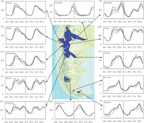
Figure 3 shows the monthly mean river flows of El Niño and La Niña composites and the long-term monthly mean river flows, with a geographical distribution of basins for the interpretation of results in a regional context. Rivers are listed from north to south, as in Table 1, and grouped according to the similarities of the annual cycle and the ENSO influence in the river flows.

Figure 3. Monthly mean river flows (m³ s⁻¹) of El Niño (red) and La Niña (blue) composites, and long-term monthly mean river flows (black), with geographical reference of the basins. The 24-month period runs from January of the year when the ENSO event starts (o) until December of the following year (+), both years separated by a vertical line.

4.1 Colorado River

The annual cycle of the Colorado River has a maximum in December and a prolonged minimum between March and September. The response to ENSO during year(o) shows, at the beginning, El Niño river flows that are below the long-term mean (l.t.m. hereinafter). By the end of year(o), El Niño river flows exceed the l.t.m. river flows, and continue thus until the mid-part of year(+). In contrast, La Niña river flows are below the l.t.m. from November of year(o) up to the first half of year(+).

4.2 Neuquén and Limay rivers

The annual cycle of the Neuquén and Limay rivers presents a maximum in November and a minimum in April, with a relative maximum in June–July and a relative minimum in September. The El Niño river flows are above the l.t.m. in the period from the second half of year(o) to the beginning of year(+), while the La Niña river flows are below the l.t.m. for the same period. The ENSO anomalies are larger around the mid-year maximum than around the late year maximum.

4.3 Cautín, Toltén and Pilmaiquén rivers

These three rivers have an annual cycle with the maximum in July and the minimum in March–April, and the ENSO signal exhibits similarities with the previous group (Section 4.2). The El Niño river flows exceed the l.t.m. river flows during the second half of year(o), while La Niña river flows are below the l.t.m. for most of year(o). For year(+), both El Niño and La Niña composites are below the l.t.m. river flows, particularly in the Pilmaiquén River.

4.4 Manso and Futaleufú rivers

The annual cycle of the Manso and Futaleufú rivers presents the maximum split in two, June–July and November, with a minimum in March and another relative minimum in September. There is a clear signal with El Niño river flows above the l.t.m. from April until the end of year(o), while in year(+), with the exception of July, river flows are below the l.t.m. The behaviour of La Niña river flows is more complex; they are below the l.t.m. in year(o), and at the beginning of year(+) there seems to be a 1-month lag with respect to the l.t.m. As a consequence, in year(+), La Niña river flows are above the l.t.m. between January and March and below the l.t.m. thereafter.

4.5 Chubut River

The annual cycle of the Chubut River has the maximum in October and the minimum in March, with relative maximum and minimum in August and September, respectively. In year(o), La Niña river flows are below the l.t.m., particularly during the third quarter of the year. The El Niño river flows show only a weak signal of above the l.t.m. in the last quarter of year(o). In year(+) the ENSO signal becomes erratic and both El Niño and La Niña switch sign during periods of a few months.

4.6 Santa Cruz River

The annual cycle of the Santa Cruz River has the maximum in March and the minimum in September. In year(o), El Niño river flows are slightly below the l.t.m. and La Niña river flows slightly above the l.t.m. In year(+), La Niña river flows are significantly below the l.t.m. around the period of annual maximum river flows between February and May, while El Niño river flows are above the l.t.m. from March on.

4.7 San Juan and Grande rivers

The annual cycle of these rivers presents the maximum in October and the minimum in February–March. La Niña river flows are below the l.t.m. during year(o), more clearly in the Grande River until October. From then on, the La Niña signal reverses to above the l.t.m. until March(+) when it is below the l.t.m. again. In contrast, El Niño river flows do not depart significantly from the l.t.m.

5 Discussion of results

We apply Student’s t test of the difference of means, as described in Section 3, in order to establish the robustness of the monthly mean ENSO departures from the l.t.m. river flows. The results are presented in coloured boxes in Tables 3 and Tables 4, in which the red scale means positive and the blue scale means negative departures, with confidence levels 99%, 95% and <95%. We consider the results as statistically significant if they satisfy at least the 95% confidence level. Although the lightest coloured box of each scale indicates least significance, it is not negligible, in particular when several consecutive months show departures of the same sign.

Analysis of the results from a geographical perspective facilitates the understanding of the response of river flows to ENSO. In Tables 3 and 4 the rivers are listed from north to south and the horizontal thick lines separate groups of rivers. The first three rivers form Group 1, as they have large basins that drain into the Atlantic Ocean, while the next five rivers, Group 2, have much smaller basins that drain into the Pacific Ocean. These eight rivers, along with the Chubut River, which drains into the Atlantic Ocean, form the group of rivers of the northern part of the region. The last three rivers, Group 3, form the group of rivers of the southern part of the region: the Santa Cruz River with a large basin draining into the Atlantic Ocean, and the San Juan and Grande rivers, with much smaller basins draining into the Pacific and Atlantic oceans, respectively.

Table 3. Differences between El Niño and long-term monthly mean river flows. The red scale boxes indicate positive differences and the blue scale boxes negative differences. The colour scale indicates that the result of Student’s t test of the difference in means is significant at 99%, 95% and <95% confidence levels, respectively. White boxes indicate no difference between monthly mean river flows. The vertical black line divides year(o) when the ENSO event begins and the following year(+). The rivers are listed from north to south and the horizontal thick lines separate groups of rivers (see text for the details).

Table 4. Differences between La Niña and long-term monthly mean river flows. See Table 3 for explanation.

At first glance, Tables 3 and 4 reveal that all rivers of the northern part (Groups 1, 2 and the Chubut River) have predominantly El Niño above and La Niña below l.t.m. river flows in the second half of year(o), in particular with higher significance level during El Niño. In year(+) the ENSO signal reverses to El Niño below and La Niña above l.t.m. river flows, particularly for Group 2 and the Chubut River, with higher significance levels in the case of La Niña. The ENSO signal of El Niño above and La Niña below l.t.m. river flows in year(o) for Group 1 rivers is prolonged during the first part of year(+), in particular in the Colorado River, in contrast to Group 2 rivers where the signal changes phase. The Group 3 rivers in the south present rather contrasting results in comparison with the northern group of rivers. The Grande and San Juan rivers show above l.t.m. river flows with both El Niño and La Niña around the transition between years, although with low significance level, while towards the end of the period the signal becomes more erratic. The Santa Cruz River shows contrasting results during El Niño in comparison with the other two rivers, i.e. below l.t.m. river flows during year(o) and above l.t.m. river flows during most of year(+). In the case of La Niña, the results are rather erratic for year(o), but from February to June of year(+) river flows are below l.t.m. with high significance level. Later on in year(+), the La Niña signal reverses to above l.t.m. river flows, with the highest significance level in October and November.

In terms of the annual cycle, the river response during ENSO events can be clearly seen at the time of maximum river flows during year(o), with the exception of the Colorado River where maximum river flows occur during the transition between years. The ENSO departures from the l.t.m. river flows are present at the time of both relative maxima, in June/July due to rainfall and in October/November due to snowmelt, in the Neuquén, Limay, Chubut, Manso and Futaleufú rivers. In the northern group of rivers, the magnitude of El Niño and La Niña departures from the l.t.m. is similar at the time of maximum river flows during year(o). In the southern group of rivers, La Niña departures from the l.t.m. are quite evident, in contrast to El Niño river flows which are less clear. In year(+), ENSO departures from the l.t.m. river flows are in general much smaller than those of year(o), with the exception of the Santa Cruz River. In the case of rivers with important nival and glacier contributions, for example the Colorado and the Santa Cruz rivers, the response to ENSO is more complex because of the relative contribution of wintertime precipitation and warm season temperature anomalies. However, the resulting effect is seen at the time of the only annual river flows maximum.

A simple way to evaluate the strength of the ENSO signal, combining geographical extent and duration, can be to count the number of river/month boxes with statistically significant differences with respect to the long-term mean. There are 288 river/month boxes in each table, i.e. 24 months × 12 rivers. In the case of El Niño, 23% of the river/month boxes (67 out of 288 boxes, Table 3) achieve the 95% confidence level, compared to 19% of La Niña (55 out of 288 boxes, Table 4). The 99% confidence level is achieved by El Niño river flows in 12% of the river/month boxes, in comparison to 4% for La Niña river flows. In terms of the sign of the departure, the statistically significant El Niño anomalies at the 95% confidence level are 87% positive and 13% negative (Table 3), while in the case of La Niña, they are 35% positive and 65% negative (Table 4). Therefore, in general, the ENSO effect is more robust with El Niño than with La Niña, with a relationship of the type El Niño/above and La Niña/below long-term monthly mean river flows.

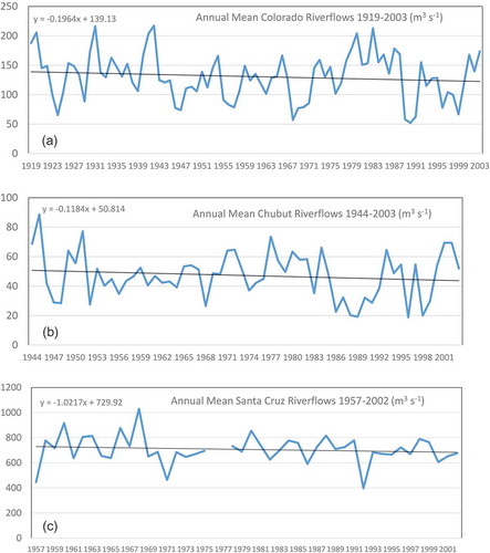
We analysed the time series of river flows with the purpose of determining possible long-term trends that could weaken the obtained results. Three rivers were selected, the Colorado, Chubut and Santa Cruz in the northern, central and southern parts of the region, respectively. These three rivers provide a good representation of the whole study region since they have large basins with different annual river flow cycles, as can be appreciated in Figure 1. Figure 4 presents the time series of annual mean river flows and it can be seen that the three rivers display a predominantly linear long-term negative trend. These linear trends can be expressed as the following changes in annual mean river flows for the whole period: 16 m³ s⁻¹ in 84 years for the Colorado River; 7 m³ s⁻¹ in 47 years for the Chubut River, and 60 m³ s⁻¹ in 52 years for the Santa Cruz River. These values represent an end-to-end change in the annual mean river flows relative to the long-term annual mean values of 12.2%, 14.6% and 6.5% for the Colorado, Chubut and Santa Cruz, respectively. We consider that the relatively small change in annual mean river flows, in comparison to the inter-annual variability displayed in Figure 4, has no significant effect on the results, so that the applied methodology is appropriate for the analysis.

Figure 4. Time series of annual mean river flows (m³ s⁻¹) of the (a) Colorado, (b) Chubut and (c) Santa Cruz rivers for the whole available period of each river.

It is important to take into consideration that there are occasions when a particular ENSO event initiated in year(o) is followed during year(+) by another ENSO event of the same phase, i.e. warm/warm or cold/cold, or opposite phase, i.e. cold/warm or warm/cold. Table 2 shows that 1905, 1911, 1924, 1925, 1939, 1951, 1954, 1964, 1965, 1970, 1972, 1973, 1976, 1983, 1988, 1995 and 1998 appear in both lists of El Niño and La Niña events. In these cases, the interpretation of results during year(+) can be questionable after a few months since the river flow conditions may not be strictly reflecting the ending of the particular El Niño or La Nina event, but also the influence of another event on its way. A similar situation may occur during the first months of year(o) because of the decay of a previous ENSO event. Therefore, the association of river flow anomalies with the occurrence of a particular ENSO phase should be restricted to the period between the last months of year(o) and the first months of the following year, in order to minimize the potential influence of another ENSO event in consecutive years. In this sense, the results are representative of the ENSO influence in the studied rivers; Tables 3 and 4 show that the statistically significant anomalies are predominantly concentrated in a period of a few months around the transition between years.

Despite the consensus of the scientific community in recognizing ENSO as a major climate driver, there are certainly other drivers of long-term variability. For example, Garreaud et al. (2009) analysed the main features of South American climate variability and indicated that the Pacific Decadal Oscillation (PDO) produces precipitation anomalies similar to those of ENSO, but with smaller amplitude. They also showed that the Antarctic Oscillation (AAO) is another source of low-frequency variability, and reported AAO-related precipitation anomalies in southern Chile and along the subtropical east coast of the continent.

6 Conclusions

Considering the combination of geographical extent and duration, the ENSO influence in the analysed group of rivers of the extreme south of South America is, in general and predominantly, stronger during El Niño than during La Niña, with a relationship of the type El Niño/above and La Niña/below long-term monthly mean river flows. With respect to the timing of the signal, the significant El Niño anomalies are concentrated in the second half of the first year, while the significant La Niña anomalies occur mainly during the first half of the second year, although less extended in time. With respect to the mean annual cycle, the ENSO signal is present, in most rivers, at the time of the high flows, and in some cases at the time of low flows, in either the first or the second year. In terms of the spatial distribution of the ENSO anomalies, the El Niño signal is stronger in the group of rivers of the northern part of the region and weakens southwards, while the La Niña signal, although weaker, does not show a particular regionality. However, we must point out that the lower strength of the ENSO signal in the southern part of the region could be due, in part, to the shorter time series of data available, in comparison to the rivers of the northern part, as this contributes to weaken the statistical significance. Nowadays, the occurrence of ENSO events is forecast and widely announced several months in advance. Therefore, the results obtained in this study can be of utility for water resources operators in the region, and the community in general, to have a perspective of a probable scenario for the upcoming months or season and eventually plan in accordance.

Acknowledgments

The authors acknowledge Engineer Gustavo Devoto, from Ente Nacional de Regulación de Energía of Argentina, for his contribution with the cartographic material and enriching discussions; and Licenciado Joaquín Aguirre, from Dirección Nacional de Aguas de Chile, for providing the data of the Chilean rivers. The authors also acknowledge the fruitful comments and suggestions made by Peter Waylen and another anonymous reviewer that contributed to improve the quality of the paper. Part of the results shown form the graduation thesis of EB at Departamento de Ciencias de la Atmósfera y los Océanos, Universidad de Buenos Aires, Argentina.

Disclosure statement

No potential conflict of interest was reported by the authors.

Additional information

Funding

GB acknowledges the partial support from research grant PICT2012-1667 of Agencia Nacional de Promoción Científica y Tecnológica of Argentina.

Notes

¹ See for example, http://origin.cpc.ncep.noaa.gov/products/analysis_monitoring/ensostuff/ONI_v5.php.

References

- Absalon, D. and Matysik, M., 2007. Changes in water quality and runoff in the Upper Oder River Basin. Geomorphology, 92, 106–118. doi:10.1016/j.geomorph.2006.07.035
- Amarasekera, K.N., et al., 1997. ENSO and the natural variability in the flow of tropical rivers. Journal of Hydrology, 200, 24–39. doi:10.1016/S0022-1694(96)03340-9
- Araneo, D. and Compagnucci, R.H., 2008. Atmospheric circulation features associated to Argentinean Andean rivers discharge variability. Geophysical Research Letters, 35, L01805. doi:10.1029/2007GL032427
- Berri, G.J. and Flamenco, E., 1998. Seasonal volume forecast of the Diamante River, Argentina, based on El Niño observations and predictions. Water Resources Research, 35, 3803–3810. doi:10.1029/1999WR900260
- Berri, G.J., Ghietto, M.A., and García, N.O., 2002. The influence of ENSO in the flows of the Upper Paraná River of South America over the past 100 years. Journal of Hydrometeorology, 3, 57–65. doi:10.1175/1525-7541(2002)003<0057:TIOEIT>2.0.CO;2
- Chiew, F.H.A., et al., 1998. El Niño Southern Oscillation and Australian rainfall, streamflow and drought: links and potential for forecasting. Journal of Hydrology, 204, 138–149. doi:10.1016/S0022-1694(97)00121-2
- Chow, V.T., 1988. Applied Hydrology. Singapore: McGraw-Hill.
- Dettinger, M.D., et al., 2000. Multiscale streamflow variability associated with El Niño/Southern Oscillation. In: H.F. Diaz and V. Markgraf, eds. El Niño and the Southern Oscillation - multiscale variability and global and regional impact. Cambridge, UK: Cambridge University Press, 113–146.
- Garreaud, R., et al., 2013. Large-scale control on the Patagonian climate. Journal of Climate, 26, 215–230. doi:10.1175/JCLI-D-12-00001.1
- Garreaud, R.D., et al., 2009. Present-day South American climate. Palaeogeography, Palaeoclimatology, Palaeoecology, 281, 180–195. doi:10.1016/j.palaeo.2007.10.032
- Kiladis, G.N. and Diaz, H.F., 1989. Global climatic anomalies associated with extremes in the Southern Oscillation. Journal of Climate, 2, 1069–1090. doi:10.1175/1520-0442(1989)002<1069:GCAAWE>2.0.CO;2
- Masiokas, M.H., et al., 2010. Intra- to multidecadal variations of snowpack and streamflow records in the Andes of Chile and Argentina between 30° and 37°S. Journal of Hydrometeorology, 11, 822–831. doi:10.1175/2010JHM1191.1
- McKerchar, A.I., Fitzharris, B.B., and Pearson, C.P., 1998. Dependency of summer lake inflows and precipitation on spring SOI. Journal of Hydrology, 205, 66–80. doi:10.1016/S0022-1694(97)00144-3
- Mohsenipour, M., Shahid, S., and Nazemosadat, M.J., 2013. Effects of El Nino Southern Oscillation on the Discharge of Kor River in Iran. Advances in Meteorology, 2013, 7. doi:10.1155/2013/846397
- Mosley, M.P., 2000. Regional differences in the effects of El Nino and La Nina on low flow and floods. Hydrological Sciences Journal, 45, 249–268. doi:10.1080/02626660009492323
- Pasquini, A. and Depetris, P., 2007. Discharge trends and flow dynamics of South American rivers draining the southern Atlantic seaboard: an overview. Journal of Hydrology, 333, 385–399. doi:10.1016/j.jhydrol.2006.09.005
- Rasmusson, E.M. and Carpenter, T.H., 1983. The relationship between eastern equatorial Pacific sea surface temperatures and rainfall over India and Sri Lanka. Monthly Weather Review, 111, 517–528. doi:10.1175/1520-0493(1983)111<0517:TRBEEP>2.0.CO;2
- Rimbu, N., et al., 2004. Impacts of the North Atlantic Oscillation and the El Niño – southern Oscillation on Danube River flow variability. Geophysical Research Letters, 31, L23203. doi:10.1029/2004GL020559
- Rivera, J.A., et al., 2017. Regional aspects of streamflow droughts in the Andean rivers of Patagonia, Argentina. Links with large-scale climatic oscillations. Hydrology Research, 49, 134–149. doi:10.2166/nh.2017.207
- Ropelewski, C.F. and Halpert, M.S., 1987. Global and regional scale precipitation patterns associated with the El Nino/Southern Oscillation. Monthly Weather Review, 115, 1606–1626. doi:10.1175/1520-0493(1987)115<1606:GARSPP>2.0.CO;2
- Ropelewski, C.F. and Jones, P.D., 1987. An extension of thje Tahiti-Darwin Southern Oscillation Index. Monthly Weather Review, 115, 2161–2165. doi:10.1175/1520-0493(1987)115<2161:AEOTTS>2.0.CO;2
- Trenberth, K.E., 1997. The definition of El Niño. Bulletin of the American Meteorological Society, 78, 2771–2777. doi:10.1175/1520-0477(1997)078<2771:TDOENO>2.0.CO;2
- Trenberth, K.E. and Stepaniak, D.P., 2001. Indices of El Niño evolution. Journal of Climate, 14, 1697–1701. doi:10.1175/1520-0442(2001)014<1697:LIOENO>2.0.CO;2
- Wilks, D.S., 2011. Statistical methods in the atmospheric sciences. Cambridge, MA: Academic Press, 704.
- Yang, Z., et al., 2012. The causes of flow regime shifts in the semi-arid Hailiutu River, Northwest China. Hydrology and Earth System Sciences, 16, 87–103. doi:10.5194/hess-16-87-2012