Improved fuzzy weighted optimum curve-fitting method for estimating the parameters of a Pearson Type-III distribution

ABSTRACT

The objective of the curve-fitting method is to determine the optimal distribution by parameter estimation. The selection of the parameter estimation methods and the determination of the parameter estimation results may vary according to the different aims of the curve fitting, as well as the different accuracies and positions of the points. To solve the problem, the fuzzy weighted optimum curve-fitting method (FWOCM) was used to deal with the characters. The deficiencies of the original FWOCM were analysed, and it was found that the membership function and nomograph were unable to effectively deal with the curve fitting. An improved method and its indexes were evaluated, using effectiveness and unbiasedness as the assessment criteria, while scoring and percentage methods were chosen to comprehensively assess the statistical results. Compared with FWOCM, the results showed greater effectiveness and unbiasedness in the improved method.

KEYWORDS:

• improved fuzzy weighted optimum method
• Pearson-Type-III distribution
• hydrologic frequency analysis
• statistical performance

Editor A. CastellarinGuest editor Y. Jia

1 Introduction

Since hydrological phenomena are uncertain, the probabilistic statistical method is applied to analyse the frequency of the hydrological data. To project the scale of different kinds of water resources and hydropower engineering that will be needed in the future, hydrological design values are calculated by the frequency curve-fitting method (Beven and Binley 1992, Rao and Hamed 2000, MWR 2006, Tang et al. 2015). The essence of the curve-fitting method is to optimize the fitting effect between the curve and the hydrological points by adjusting the distributions and parameters of the curve. The distributions of the series, such as the lognormal, Gumbel, log-Pearson Type-III and generalized extreme value distribution, should be eliminated as candidates for modelling the series. Ideally, the distributions should relate to the characteristics of the region, the sequence itself and treatment of outliers, and include a large set of historical flood values, data transformation and the causal composition of the flood population (Cunnane 1985, Haktanir and Horlacher 1993, Karim and Chowdhury 1995, Sandoval and Villasenor 2008). In China, the distribution that could fit well with hydrological data has been widely researched. The Pearson Type-III (P-III) distribution and the Kriczki-Minca curve have been considered, and the results indicated that the P-III distribution fits better when the coefficient of variation, C_v, is higher. Part of the advantage of the P-III distribution is its malleability; as a result, it is widely used in China (e.g. Chen et al. 1963, Ye 1964, Jin 1964). This paper investigates the P-III distribution.

There are two major categories of hydrological frequency calculation methods (Song et al. 2008b, Li and Song 2014): numerical solution methods and curve-fitting methods. The numerical solution methods include the moment method (Wallis et al. 1974), the weight function method (Jin 2001, Liang et al. 2014), the maximum-likelihood method (Ponce 1989, Yu et al. 2012), the probability weighted moment method (Greenwood et al. 1979, Haktanir 1997), and the linear moment method (Chow and Watt 1994, Hosking and Wallace 1997, Parida et al. 1998, Kumar et al. 2003, Karvanen and Nuutinen 2008). The numerical solution methods are based on the basic theory of probability statistics for data processing to obtain the parameters of the frequency distribution with strong mathematical theory. The curve-fitting methods include the optimum curve-fitting methods and the ocular estimation methods. The optimum curve-fitting methods are based on reasonable optimum curve-fitting standards, within the scope of the constraint conditions used to determine a set of parameters. The parameters determine a theoretic frequency curve that fits well with the actual sample points. In the ocular estimation methods, the results of the numerical solution methods are chosen as the initial values, according to the actual engineering requirements and the precision and position of the points. The parameters are artificially adjusted to achieve the optimum fitting effect. These methods can reflect the difference of the weight of the points well, while the methods do not have a reliable measure, and, requiring much empirical experience, are not reliable. With the rapid development of computer technology, curve-fitting methods have been developed using reasonable optimum criteria and frequency formulas to obtain the optimum parameters. Researchers have conducted system analysis (Cong et al. 1980, Ye et al. 1981, Guo 1987), but have found it difficult to use the mathematical methods to obtain effective arguments for the optimization algorithm. They also point out that the large sample statistical test method should be used to verify the analysis. The optimization rules of the curve-fitting method (Lei et al. 2015) include the transverse and longitudinal residual sum of squares criterion and the transverse and longitudinal residual sum of absolute value criterion. At present, both criteria are widely used to calculate the design values corresponding to the frequency.

The longitudinal distance of the residual sum of squares as the objective function is very close to the least squares method. The effect of each point on the target should be different, so the weighted method is more reasonable. In the weighted least squares method, large and small-to-moderate sequence sizes have different weights (Carroll et al. 1988). The weighted least squares method, using 1/x² as a weighting factor, has been compared with the conventional ordinary and weighted least squares method, and the application demonstrates that the performance of the improved method exceeds that of the original method (Sarbu 1995). By modifying the Gaussian paradigm, an iteratively weighted least squares method has been proposed that is robust (Chatterjee and Mahler 1997). In the P-III curve-fitting method, the objective function is determined by the curve-fitting criteria and destinations. The weighted optimum curve-fitting method is able to search the parameters in the frequency analysis. To effectively enhance the ductility of the frequency curve, the precision, position and importance of the points are treated effectively by the weight. The key is to relate the weight to the size of the sample.

The weighted optimum curve-fitting method (Deng et al. 1995, Xie et al. 1997, Qiu et al. 1998, Xie and Zheng 2000) has been thoroughly researched from different angles. The accuracy and importance of the points, as well as the purpose of the curve fitting, influence the weights of the points, which are calculated by the experience formula (Xie and Zheng 2000). While there is no unified standard for the weight level, the calculation results vary from researcher to researcher. Deng et al. (1995) first proposed that the degree of uncertainty of the visualizing curve-fitting methods ought to be measured by the membership function. That is, the errors of observation data should be calculated by the trapezoidal method, and the normal distribution function should be adopted to establish the membership function of the design values and the design frequencies.

The fuzzy weighted optimum curve-fitting method (FWOCM) was studied using the statistical test method, while the estimation precision of the membership function parameters depended on the experience of hydrology workers, which was difficult to obtain effectively. In the 1990s, the FWOCM has been independently proposed by two researchers: Xie et al. (1997) and Qiu et al. (1998). Qiu et al. (1998) assumed that there was an ideal optimum curve in the curve-fitting process, and all of the known points were just right on the ideal curve. The membership function was established by the fluctuation of the deviation of the experience points from the ideal curve obeying normal distribution. The ideal data and the measured data were used to judge the curve-fitting effect. In their study, Xie et al. (1997) derived the membership function by the idea of order statistics, and the ideal data were used to judge the curve-fitting effect. The similarity in the two proposed methods (Xie et al. 1997, Qiu et al. 1998) is the calculation of the membership function parameter – the standard deviation.

The standard deviation was computed with B values from the nomograph of the Ministry of Water Resources (MWR 2006). However, the limitation of nomograph length restricts the reliability of the FWOCM. No correlation to improve the method was found in the literature. To improve the method, the nomograph and the membership function are first analysed and improved. Therefore, the new nomograph is extended. In addition, it should not be ignored that the sample size should be infinite on the mathematical statistical methods, but the hydrological sequence is not long enough. After studying the membership function, it was found that the normal distribution membership function is not the optimum membership function, and a new membership function is therefore derived.

In this study, on the basis of the improved membership function and nomograph, a new artificial intelligence algorithm, i.e. the Social Spider Optimization algorithm (SSO; Wang et al. 2015), is used to search for the best parameters. The SSO algorithm is a swarm algorithm that can find parameters with higher accuracy than other algorithms (Wang et al. 2015). Only the practical data were used to test the character of the algorithm, and the evaluation indicators and methods are simple and insufficient. In this study, the Monte Carlo statistical test is used for testing the effectiveness and unbiasedness of the curve-fitting methods. (An estimate is unbiased if its expected value equals the true parameter value.) The Monte Carlo method, on a distribution, can produce hundreds, thousands or even tens of thousands of (pseudo) random series (or samples) of the same number of years, and then apply an empirical frequency formula and a statistical parameter estimation method to obtain the mathematical average values of the parameters and design values of these series (Cong et al. 1980, Ye et al. 1981).

Improved methods have been introduced by Lei et al. (2018). However, the tests are simple and insufficient to explain the improvements of the methods (Wang et al. 2017). The statistical test results are evaluated by the assessment method and the percentage method, as described in Section 3. Our results show that the effectiveness and unbiasedness are chosen as indexes to judge the fitting effect. The measured data and the relative error line charts are used to test the improved methods.

2 Methods

2.1 Social Spider Optimization (SSO) algorithm

With the development of computer technology, more and more new soft techniques have been developed and are being used in hydrological calculations. Examples of some of these techniques are the artificial neural network (Wu and Chau 2011), bias theory (Fotovatikhah et al. 2018) and intelligent optimization algorithms (Cheng et al. 2005, Chau 2007, Taormina et al. 2015), all of which can be used to manage and search for the optimal scheme.

Techniques such as intelligent optimization algorithms have been introduced into an improved hydrological frequency parameter analysis. Examples are the ant colony algorithm (Li and Song 2009, Cao et al. 2010), the genetic algorithm (Song et al. 2008a, Wang et al. 2009), particle swarm optimization (PSO) (Yao and Song 2007, Liu et al. 2009), the simulated annealing algorithm (Chen et al. 2012), and the SSO algorithm (Wang et al. 2015), a new kind of stochastic global optimization technique (Cuevas et al. 2013). The curve-fitting method of SSO has been compared with that of the GA and PSO (Wu 2015, Wang et al. 2016), and the SSO was found to perform better than both GA and PSO, with good searching ability. The SSO (Cuevas et al. 2013) was devised by simulating the cooperation behaviours of social spiders. The individual particles used to search for the best values are separated into two categories: “male” and “female” spiders, each of which responds to different search criteria (set of different evolutionary operators) during the optimization process. The SSO search pattern effectively avoids allowing individuals to gather around others that are at an advantage and is able to perform a global search that effectively avoids premature convergence and instability of the results. Most importantly, the typical function optimization results show that the SSO is not sensitive to the initial values and the parameter selection; it is robust and its convergence speed is fast. Therefore, the SSO was applied to the numerical algorithm of adaptive P-III curve parameter estimation, and the system analysis was carried out (Wang et al. 2015); the SSO was shown to obtain good parameter searching effect. In this study, we referred to Wang et al. (2015) to obtain a detailed optimization model. The modelling steps are described briefly below, and the optimization process is shown in Figure 1.

Figure 1. Flow chart of the Social Spider Optimization (SSO) algorithm.

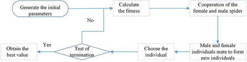
Step1: Generate the initial population. The default values of unified 200,500 data are the population size N and the largest number of iterations I_max. The threshold value PF is 0.55, and the values of the female high limit coefficient and the female low limit coefficient are P_j^high = 0.9 and P_j^low = 0.65, respectively; the mean value $\bar{x}$ is calculated by the moment method, and the values of the coefficient of variation, C_v, and the coefficient of skewness, C_s, are both between 0 and 10. The female and male individual initialization randomly generates the initial female and male spider individuals, where a spider individual represents a set of parameters. A single spider individual fitness value is calculated, and the optimum and worst individuals are obtained.

Step2: Loop iteration. The female and male spiders move in search space (public) in accordance with their respective collaborative mechanisms. They constantly change their position. The male and female spider individuals continuously produce new offspring by the “mating” mechanism.

Step3: Select the offspring. The optimization of the individuals for newly produced spiders is done by calculating the fitness values and comparing them with the optimum value of previous spiders. If the fitness values of the newly produced spiders are better than the previous optimum value, the new individuals will replace the original optimum individuals, and the current state of the new spiders will be saved.

Step4: Termination inspection. If the termination conditions are met, the calculation is stopped; if they are not met, Step 3 is repeated for the next round of iteration. The iteration is not stopped until the conditions of the termination iteration are satisfied.

2.2 Fuzzy weighted optimum curve-fitting method (FWOCM)

According to the description in the literature (Qiu et al. 1998), it is assumed that there is an ideal optimum curve on which all of the points are just right. On the basis of the proximity degree of order statistics and the ideal optimum curve, and based on the theory of fuzzy mathematics, the membership degree is introduced to establish the objective function. If the probability density function of an ideal optimum curve for a random sequence X is f(x, E_x, C_v, C_s), then the membership degree for some experience points (x_m, p_m) should be calculated by:

(1) $\mathrm{F}{\mathrm{W}}_m\left(x_m,p_m\right)=1-2\underset{b}{\overset{a}{\int }}\frac{1}{{\sigma }_m\sqrt{2\pi }}\mathrm{e}\mathrm{x}\mathrm{p}\left\{-\frac{{\left[x-x\left(p_m\right)\right]}^2}{2{\sigma }_m^2}\right\}\mathrm{d}x$(1)

and the objective function of FWOCM is:

(2) $\mathrm{m}\mathrm{i}\mathrm{n}\sum _{m=1}^n\mathrm{F}{\mathrm{W}}_m{\left|x_m-x\left(p_m\right)\right|}^c$(2)

where m is the serial number of the point; n is the total number of points; FW_m is the membership degree of the point m with the ideal curve; x_m is the true value of the point m; p_m is the frequency of point m; x(p_m) is the fitting value of the point m; a and b are, respectively, the upper and lower limit of the integral interval; σ_m is the standard deviation of the deviation between x(p_m) and x_m; and c is the power exponent of the deviation between x(p_m) and x_m.

To compare clearly with the improved methods, this model (Qiu et al. 1998) is referred to as the FWOCM or the original method.

2.3 Analysis of FWOCM

The FWOCM is tested by a set of hydrological sequences. The membership function and the nomograph are the two basic elements of the method.

The weights of the points are calculated by the numerical integration of the membership function in the integral interval. The upper and lower limits of the integral interval (a, b) are obtained by the reduction of the numerical integration as follows:

(3a) $a=\left[x_m+\mathrm{N}\mathrm{B}\left(p_m,C_{\mathrm{s}}\right)-x\left(p_m\right)\right]/\sqrt{2}{\sigma }_m$(3a)

(3b) $b=\left[x_m-\mathrm{N}\mathrm{B}\left(p_m,C_{\mathrm{s}}\right)-x\left(p_m\right)\right]/\sqrt{2}{\sigma }_m$(3b)

where NB(p_m, C_s) is the range of design value (which can be calculated by Equations (8) and (9)), and C_s is the coefficient of skewness of the sequence X.

The order of magnitude of the standard deviation, σ_m, of the design values is between 10⁻² and 10⁻³, obtained by Monte Carlo simulation. If σ_m is substituted in Equation (1), the membership degree of a point is close to the value 1, meaning that the point is just on the ideal optimum curve. Since the result is hardly convincing, the membership function should be improved.

The nomograph is the graph showing the B values corresponding to the frequency and the skewness coefficient. In the Charts of Chinese Hydrological Statistics, B values are used to calculate the standard deviation of the sampling distribution of the design values. The length of the nomograph was extended from frequency 5% to 20% by Jin and Fei (1991). However, the length of the nomograph is still limited, so points higher than 20% will not be used in the FWOCM. The frequency of the nomograph needs to be increased from 20% to 99%.

2.4 Improved model

2.4.1 Data processing

The commonly used frequency distributions are lognormal, Pareto, Pearson Type-III, log-Pearson Type-III, logistic, Gumbel and exponential distributions (Li 1984). In China, where the results of long-term flood series have been analysed and many years of practical work have gone into design work, the Pearson Type-III (P-III) curve is generally adopted in engineering design and has been standardized.

If the random variable X obeys the P-III distribution, its probability density function is as follows:

(4) $\mathrm{f}(x)=\frac{\left|\beta \right|}{\mathrm{\Gamma }(\alpha )}{\left[\beta (x-a_0)\right]}^{\alpha -1}exp(-\beta (x-a_0))$(4)

where Γ() is the gamma function, α is the shape parameter, β is the scale parameter and α₀ is the position parameter, with α = 4/C_s², β = $2/\bar{x}{C}_{\mathrm{v}}{C}_{\mathrm{s}}$, and a₀ =$\bar{x}\left(1-2C_{\mathrm{v}}/C_{\mathrm{s}}\right)$.

To exclude the influence of the order of magnitude on weight, in this paper, the data have been transformed. According to the different sources of original data, these transformation methods can be divided into three categories: subjective weighting, objective weighting and combination weighting. In this paper, the normalization process is the objective weighting method. This method is simple and allows the computer program to do a statistical experiment without special points or expert knowledge.

(5) $x_{0i}=x_i/\bar{X}$(5)

where x_i is the elements in vectors X = (x₁, x₂, …, x_n), $\bar{X}$ is the mean of the sequence X, and x_0i is the new sequence.

This calculation easily proves that the characteristic values, C_v and C_s, will not change after the transformation. Equation (1) can be changed to study $A=\underset{b}{\overset{a}{\int }}exp\left(-x^2\right)\mathrm{d}x$. From the experiment, we can see that if x is larger than 5, A is 3.6 × 10⁻¹¹, that is, A is very small. If the data do not change by Equation (5), the points with greater degree of error membership may be closed with 1, so that the weights are unable to effectively distinguish the importance of the points. The transformation may enable the weights to more accurately distinguish the importance of the points.

2.4.2 Improvement of the membership function

The frequency analysis is made on the basis of a large capacity sample. If the sample size n approaches infinity, the value of the formula ${\sigma }_m=S/\sqrt{n}B$ will be changed, that is, ${\sigma }_m\to 0$. The length of the observed hydrological sequence is limited, so the capacity n is limited. The substitution method is used by $X=\sqrt{2}{\sigma }_m\cdot X$ to exclude the disturbance of the standard deviation σ_m in the integral problem. This calculation proves that the falling semi-normal distribution should be the membership function distribution, as follows (Lei et al. 2018):

(6) $\mathrm{F}{\mathrm{W}}_m\left(x_m,p_m\right)=1-2\underset{b}{\overset{a}{\int }}\frac{1}{\sqrt{\pi }}\mathrm{e}\mathrm{x}\mathrm{p}\left\{-{\left[x-x\left(p_m\right)\right]}^2\right\}\mathrm{d}x$(6)

where $a=x_m\vee x\left(p_m\right)$ and $b=x_m\wedge x\left(p_m\right)$.

It is assumed that the distribution of both sides of the estimated value of each frequency point is normal (Xie et al. 1997, Qiu et al. 1998). The confidence probability (1 – α) is used to calculate the interval estimate value of the design value (Cong et al. 1980). The upper and lower bounds of the confidence interval are:

(7a) $a=x_m+\mathrm{N}\mathrm{B}\left(p_m,C_{\mathrm{s}}\right)-x\left(p_m\right)$(7a)

(7b) $b=x_m-\mathrm{N}\mathrm{B}\left(p_m,C_{\mathrm{s}}\right)-x\left(p_m\right)$(7b)

with

(8) $\mathrm{N}\mathrm{B}\left(p_m,C_{\mathrm{s}}\right)=\sigma /\sqrt{n}\cdot z_{\alpha /2}$(8)

and

(9) $\sigma =S/\sqrt{n}\cdot B$(9)

where $z_{\alpha /2}$ represents the corresponding quantile of the normal distribution, whose frequency is $\alpha /2$ (in this paper α = 0.05, $z_{\alpha /2}$ = 1.96); S is the standard deviation of the series; and B is the value that is checked from the nomograph by the frequency of the design values and the coefficient of skewness. The skewness coefficient C_s is sensitive; if C_s is very high, the lower part of the curve is too flat and has a poor fit with small values, and if C_s is greater than 2, we cannot get suitable parameters for the floods of small and medium-sized rivers in arid and semi-arid regions.

2.4.3 Improvement of the nomograph

The nomograph drawing has been studied extensively (Cong et al. 1980, Jin and Fei 1991, Liu et al. 2006). On the basis of Jin and Fei (1991), the nomograph is improved with the Monte Carlo and optimization method in this study. The nomograph B value is calculated by the statistical method with random data which obeys the P-III distribution. Equation (9) is transformed to $B=\sigma \sqrt{n}/S$ to calculate the nomograph B value, where S is the standard deviation of the random sequence that corresponds to the coefficient of skewness, C_s, and σ is the standard deviation of the point that corresponds to C_s and the frequency of the design value. The new-modified nomograph B values are listed in Table 1 (Wang et al. 2017, Lei et al. 2018).

Table 1. Modified nomograph B values of least squares method.

Cs	p (%)
	0.01	0.1	1	5	10	20	30	40	50	60	70	80	90	99
0	3.2	2.6	2.0	1.6	1.4	1.2	1.1	1.0	0.9	0.9	0.8	0.8	0.8	0.7
0.5	7.2	5.2	3.4	2.3	1.9	1.5	1.3	1.2	1.1	1.0	0.9	0.9	0.8	0.8
1	11.2	7.6	4.6	2.9	2.3	1.8	1.5	1.3	1.2	1.1	1.0	0.9	0.8	0.8
1.5	16.1	10.6	6.2	3.8	3.0	2.2	1.9	1.6	1.4	1.3	1.1	1.1	1.0	0.9
2	30.6	19.0	10.2	5.8	4.3	3.0	2.4	2.0	1.7	1.5	1.3	1.2	1.1	1.0
2.5	36.0	21.6	11.1	6.0	4.3	2.9	2.2	1.8	1.5	1.3	1.2	1.0	0.9	0.8
3	42.9	25.3	12.6	6.5	4.5	3.0	2.2	1.8	1.5	1.3	1.1	1.0	0.9	0.8
3.5	55.3	30.9	14.1	6.7	4.5	2.8	2.1	1.6	1.3	1.1	0.9	0.8	0.7	0.6
4	58.4	32.0	14.2	6.4	4.2	2.5	1.8	1.3	1.1	0.9	0.8	0.6	0.6	0.5
4.5	60.8	33.2	14.5	6.4	4.1	2.4	1.6	1.2	1.0	0.8	0.6	0.5	0.5	0.4
5	67.2	35.8	15.0	6.3	3.9	2.2	1.4	1.1	0.8	0.6	0.5	0.4	0.4	0.3
5.5	73.0	38.0	15.2	6.0	3.6	1.9	1.2	0.9	0.6	0.5	0.4	0.3	0.3	0.2
6	93.8	47.6	18.2	6.8	3.8	1.9	1.2	0.8	0.6	0.4	0.3	0.3	0.2	0.2

2.4.4 Objective function

The membership degree value of each frequency point indicates the degree of fluctuation between the design value and the ideal optimum value, specifies the uncertainty of the point in the curve-fitting process, and reflects the importance of the point in the curve fitting. The membership degree $\mathrm{F}{\mathrm{W}}_m\left(x_m,p_m\right)$ is greater than 0 and less than 1. To illustrate the magnitude of the fluctuation of one point in the overall sequence, the normalization process is conducted to transform the uncertainty value into a weight, as follows:

(10) $s_m=\frac{\mathrm{F}{\mathrm{W}}_m\left(x_m,p_m\right)}{{\sum }_{m=1}^n\mathrm{F}{\mathrm{W}}_m\left(x_m,p_m\right)}\left(m=1,2,\dots n\right)$(10)

where s_m is the weight of the point whose frequency is p_m; $\mathrm{F}{\mathrm{W}}_m\left(x_m,p_m\right)$ is the uncertainty of the point; and n is the length of the sequence.

The optimization criteria are divided into two parts: (i) the horizontal and vertical sum of squares of deviations, and (ii) the horizontal and vertical sum of the absolute sum of deviations (Ge 1990). The vertical residual is used as the objective function for the frequency as the index. The horizontal sum of squares of deviations has been widely used.

The objective function, T, is obtained as follows:

(11) $T=\sum _{m=1}^n{s}_m{\left[x_m-x\left(p_m\right)\right]}^2$(11)

2.5 Stages of modelling

In this paper, the data are either random or measured. The random data are generated by the Monte Carlo method, and the measured data are from the engineering hydrology books. The FWOCM modelling steps – with either the random or measured data – are as follows, and summarized in Figure 2.

Figure 2. Flow chart of the fuzzy-weighted optimum curve-fitting method (FWOCM).

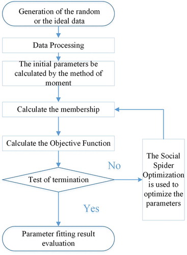
Step1: Set the initial values. The known data series are sorted in descending order to calculate the frequency of each point by the mathematical expectation formula (that is the Weibull formula). The mean x_m, the coefficient of variation C_v, and the coefficient of skewness C_s are calculated by the method of moments after data processing. Then, the calculated parameters are discretized on the basis of the step sizes. The ranges of the parameters are taken as the initial values.

Step 2: Determine the range of integration. Equation (9) is used to calculate the value of σ_m and Equations (7a) and (7b) are used to calculate the integral interval, which is the confidence interval of the falling semi-normal distribution.

Step 3: Calculate the objective function. The objective function values of different frequencies are, respectively, computed by the membership function (Equation (6)) and the weight calculation (Equation (10)) in order to calculate the uncertainty and the weight value of each point.

Step 4: Optimize the parameters. The objective function is established by Equation (11). The SSO algorithm is used to search for the best parameters, such as C_v and C_s.

Step5: Evaluate the results. The results that meet the iteration termination conditions are evaluated.

3 Experiment

The improvements of the FWOCM were introduced in Section 2.4. An experiment is introduced to evaluate the performance of the improved method against the original method. Here, we include the design of the experimental scheme, the evaluation criteria, the evaluation of the random data and the measured data, the results, and the discussion.

3.1 Design of the experimental scheme

The Monte Carlo method is used to generate the groups of random data that obey the P-III distribution as the test data. The random data generated by a computer are pseudo-random data that obey statistically significant Pearson Type-III distribution. The sample data in Qiu et al. (1998) are generated based on the parameters and the following formula:

(12) $X_p=\bar{x}(1+C_{\mathrm{v}}{\mathrm{\Phi }}_p)$(12)

where $\bar{x}$ is the mean; and ${\mathrm{\Phi }}_p$ is a function of C_v and the design frequency p. To be relative to the ideal data that strictly obey the P-III distribution in Qiu et al. (1998), the mean value is set at EX₀ = 1.0, the coefficients of variation, C_v0 are 0.5, 0.75, 0.67 and 1, and the coefficients of skewness, C_s0 are 0.625, 1, 1.5, 2 and 3. The capacities of the sequences are, respectively, set as 19 and 29. After the random data are generated, the objective function is established by the transverse residual sum of squares criterion. There are 40 schemes that correspond to the sequences generated by the parameter groups. The schemes are used to calculate the theoretical values. The theoretical values are used to evaluate the improved FWOCMs by different evaluation criteria. The total number of statistical tests of each parameter group is 1000.

3.2 Evaluation criteria

In the optimum curve-fitting methods, the fitting effect is evaluated by the transverse and longitudinal residual sum of squares, and the transverse and longitudinal residual sum of absolute values. These indexes are regarded as the standards for judging the merits of the fitting effect. Additionally, the actual sample values and theoretical values are drawn on the coordinate graph, so the merits of the fitting effect can be observed and judged. (The actual sample values represent the random data and the measured data.)

The purpose of the FWOCM is to measure the uncertainty of the actual sample values that have sampling errors and to enhance the effect of the extension of the hydrological frequency curve. The FWOCM is combined with the weight and the deviation as the objective function, but neither the transverse and longitudinal residual sum of squares nor the transverse and longitudinal residual sum of absolute values clearly reflect the effect of the weight. Therefore, the index of the ductility of the hydrological frequency curve is used as an evaluation criterion to measure the effect of the FWOCM on the random data. This index measures the unbiasedness and effectiveness of the theoretical values of once in a million years, once in a thousand years, once in a hundred years, and once in 10 years. Since the measured data cannot be used to evaluate the extrapolation ability of the FWOCM, the fitting errors of the measured values, the theoretical values matched to specific points are used to judge the advantage of FWOCM.

The unbiasedness and effectiveness of the theoretical values are, respectively, calculated by the mean relative deviation, B_xp and the relative root-mean-square error S_xp (Yang and Ding 1988, Chen and Hou 1992, Liang et al. 2001). The mean relative deviation B_xp is used to characterize the deviation between the actual sample values and the theoretical values. The smaller the B_xp, the better the unbiasedness of the method. The relative root-mean-square error, S_xp is used to characterize the volatility of the fitting degree of the different sequences. The smaller the S_xp, the lower volatility of the method.

(13) $S_{\mathrm{x}\mathrm{p}}=\frac{1}{N}\sqrt{\sum _{i=1}^{N_{\mathrm{s}}}{({{\hat{x}}^i}_p-x_p^0)}^2/{(x_p^0)}^2}\times 100\mathrm{\%}$(13)

(14) $B_{\mathrm{x}\mathrm{p}}=\frac{\sum _{i=1}^{N_{\mathrm{s}}}({{\hat{x}}^i}_p-x_p^0)}{N{x}_p^0}\times 100\mathrm{\%}$(14)

where p is the design frequency; $x_p^0$ and ${{\hat{x}}^i}_p$ are, respectively, the overall actual sample value corresponding to p, and the estimated (theoretical) value of the actual sample value corresponding to p; and N is the number of tests.

After the parameters are determined, the unbiasedness and effectiveness of theoretical values corresponding to the frequency p = 0.01%, 0.1%, 1%, 10% are calculated. Based on the four values of the 40 schemes, the B_xp and S_xp are calculated.

3.3 Evaluation of the random data results

To evaluate the results, the mean and standard deviation of the offset of each group, i.e. the distribution of the offset, are calculated. A single criterion cannot reflect the difference between the methods. To evaluate the different methods, a range of assessment tools provides the researcher with several options: comprehensive evaluation methods, such as the analytic hierarchy process (AHP), the fuzzy comprehensive evaluation method (FCE), the rank sum ratio (RSR), the composite index method, or the technique for ordering preference by similarity to an ideal solution, may be used to evaluate the different indexes (Jia et al. 2008). While each of the methods has its own application scope, which cannot be used in the statistical tests, the scoring method and the percentage method are the best choices.

3.3.1 Scoring method

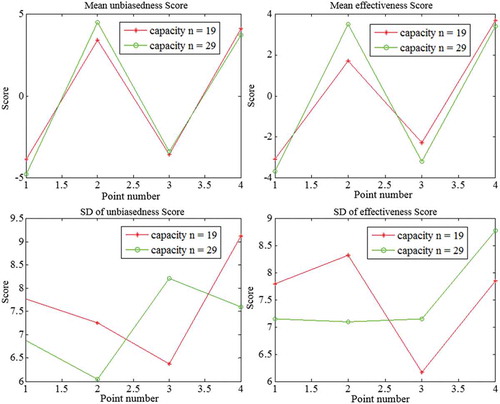
On the basis of improvement in the nomograph and membership function of FWOCM, three new methods are generated: the Optimization of the Membership Function FWOCM (OMF-FWOCM), the Optimization of the Nomograph FWOCM (ON-FWOCM), and the Optimization of the Membership Function and Nomograph FWOCM (OMFN-FWOCM). With 40 values corresponding to each frequency (p = 0.01%, 0.1%, 1%, 10%) in each experiment, the unbiasedness and effectiveness of the values are calculated. To effectively analyse the performance of the proposed methods, the evaluation indexes of the theoretical values corresponding to each frequency are compared. The smaller of the two methods is assigned 1 point, the larger is assigned –1, and if they are equal, both methods receive 0. In each experiment, the final score is the summary of the four values of each method. For the sequence size of 19 or 29, each method receives 1000 values. The mean and the standard deviation are calculated using the 1000 values. The final results are presented in Table 2 and Figure 3.

Table 2. Comparison of the relevant value score by different methods. M: mean; SD: standard deviation.

Sample size	Characteristic value	Method
		FWOCM		OMF-FWOCM		ON-FWOCM		OMFN-FWOCM
		M	SD	M	SD	M	SD	M	SD
19	Unbiasedness	–3.9	7.77	3.4	7.26	–3.6	6.38	4.1	9.12
	Effectiveness	–3.1	7.80	1.7	8.32	–2.3	6.17	3.7	7.85
29	Unbiasedness	–4.8	6.88	4.5	6.05	–3.4	8.21	3.7	7.60
	Effectiveness	–3.7	7.15	3.5	7.10	–3.2	7.15	3.4	8.78

Figure 3. Comparison of the relevant value scores by different methods. SD: standard deviation. Point numbers: 1 – FWOCM, 2 – OMF-FWOCM, 3 – ON-FWOCM and 4 – OMFN-FWOCM.

3.3.2 Percentage method

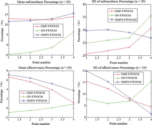
To further analyse the performance of the improved methods, the relative errors are taken as indexes to compare the degree of improvement in the unbiasedness and effectiveness between the original method and the improved methods. Thus, OMF-FWOCM, ON-FWOCM, and OMFN-FWOCM are compared with FWOCM. Each experiment calculates 40 relative errors of unbiasedness and effectiveness to one of the improved FWOCMs compared with the original FWOCM. Finally, the mean and standard deviation are calculated with relative errors of 1000 groups in unbiasedness and effectiveness. The results are listed in Table 3, while Figures 4 and 5 show contractions in the characteristic values, based on the improved percentage in relative error of the different frequencies, for the capacities 19 and 29, respectively.

Table 3. Mean (M) and standard deviation (SD) of unbiasedness and effectiveness of the improved frequency percentages by different methods for sequence sizes (capacities) 19 and 29. Positive values represent improvement compared with the original method, while negative values represent worsening compared with the original method.

	Frequency	Statistic	Method
			OMF-FWOCM	ON-FWOCM	OMFN-FWOCM
Capacity: 19
Unbiasedness	0.01%	M	8.63	–7.51	17.24
		SD	31.05	22.82	25.52
	0.1%	M	8.45	–5.71	18.10
		SD	31.52	20.75	26.36
	1%	M	7.66	–2.21	19.29
		SD	33.22	16.96	27.18
	10%	M	3.82	6.53	20.95
		SD	44.73	14.66	30.74
Effectiveness	0.01%	M	2.99	–0.87	6.34
		SD	17.37	11.80	10.60
	0.1%	M	2.60	–0.23	5.67
		SD	15.53	9.81	9.95
	1%	M	1.93	0.61	4.47
		SD	12.40	7.54	8.70
	10%	M	0.91	1.11	2.12
		SD	8.01	8.16	7.58
Capacity: 29
Unbiasedness	0.01%	M	12.91	–4.65	11.58
		SD	20.63	24.82	29.72
	0.1%	M	12.59	–3.68	11.93
		SD	21.82	25.99	30.11
	1%	M	12.32	–1.36	12.84
		SD	23.22	26.90	29.01
	10%	M	13.97	6.41	15.63
		SD	30.76	35.63	26.88
Effectiveness	0.01%	M	6.65	–0.96	7.14
		SD	11.07	9.56	11.97
	0.1%	M	5.61	–0.57	6.40
		SD	10.45	9.18	11.05
	1%	M	3.89	0.01	5.19
		SD	9.50	9.39	9.66
	10%	M	1.13	0.84	3.70
		SD	8.89	11.10	8.28

Figure 4. Mean and standard deviation (SD) of improved percentages in unbiasedness and effectiveness for sample size n = 19.

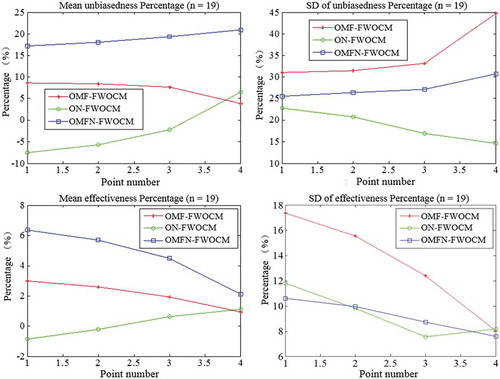
Figure 5. Mean and standard deviation (SD) of improved percentages in unbiasedness and effectiveness for sample size n = 29.

The relative error, R_yp, is calculated by:

(15) $R_{\mathrm{y}\mathrm{p}}=\frac{y_p^i-y_p^0}{y_p^0}\times 100$(15)

where $y_p^i$ is the unbiasedness and effectiveness of the improved method, and $y_p^0$ is the unbiasedness and effectiveness of the original method.

In Figures 4 and 5, points 1 to 4 represent p= 0.01%, 0.1%, 1% and 10%, respectively.

3.4 Evaluation of the measured data results

The curve-fitting methods for general floods and catastrophic floods are different. One difference is that the frequencies of the overall points are calculated according to different frequency formulas, while a second difference is that the existence of a catastrophic flood directly affects the accuracy of the curve’s fitness values. Catering to catastrophic flood points in the curve-fitting can make the whole curves appear very high. However, if the existence of a catastrophic flood is not considered, the optimum curve parameters will lose credibility. Despite these limitations, the weighted curve-fitting method is a good way to deal with the problem of a catastrophic flood, a topic of great interest in hydrology. Therefore, the FWOCM is applied to general and catastrophic floods to provide a new way to solve the problem.

In the literature, hydrological sequences are considered (e.g. Song and Ma 2009, Wang et al. 2013), and the methods listed above are used to, respectively, calculate the corresponding parameter values, as well as each deviation of the theoretical values from the measured values. The percentages of the fitting deviation for general floods and catastrophic flood are calculated, and the statistical test results are shown in Table 4. Series 1, 2, 3 and 4 represent the general flood sequences, and series 5 and 6 represent the catastrophic flood sequences.

Table 4. Mean (M) and standard deviation (SD) of the fitting deviation percentages with actual-measured sequences of general floods (series 1–4) and catastrophic floods (series 5 and 6) using the original and improved methods.

Series	Statistic	Method
		FWOCM	OMF-FWOCM	ON-FWOCM	OMFN-FWOCM
1	M	–1.25	1.08	–0.42	0.58
	SD	2.66	2.73	1.25	1.18
2	M	–1.06	0.16	–0.16	1.06
	SD	2.56	2.18	1.24	2.34
3	M	–0.17	0.24	0.09	0.05
	SD	4.34	3.83	2.44	2.38
4	M	–0.57	0.12	0.58	0.12
	SD	4.04	2.81	4.63	2.81
5	M	–0.56	–0.56	–0.56	1.69
	SD	2.08	1.41	2.72	1.73
6	M	–0.38	0.17	–1.48	1.69
	SD	1.70	2.48	1.74	1.79

A line chart is made on the basis of the fitting deviation. The purpose of the chart is threefold: first, to observe the hydrological sequence fitting errors of the different methods; second, to observe the fluctuations of the fitting degrees according to the frequencies of the sequence points; and third, to judge the inflection points of the different methods and fitting effects. Figures 6 and 7 show the improved percentage characters of the hydrological sequence points of the different frequencies. Using the fitting curves of four methods on general and catastrophic flood sequences, the fitting effect can be analysed directly (Figs. 8 and 9).

Figure 8. Fitting curves of four methods for four general flood sequences.

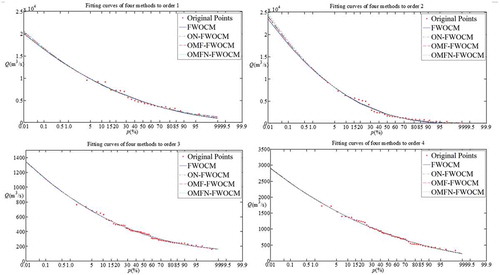
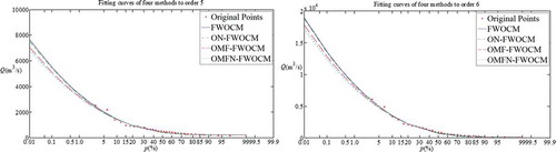
Figure 9. Fitting curves of four methods for two catastrophic flood sequences.

4 Analysis of the results and discussion

4.1 Random data

To test the function of the improved methods, the Monte Carlo method is used both to run the experiment and to first generate the random data. The scoring method and the percentage method are then used to evaluate the indexes of unbiasedness and effectiveness.

4.1.1 Comparing original and improved methods

As shown in Table 2 and Figure 3, by comparing the original and improved methods, the unbiasedness and effectiveness of the corresponding improved methods increased. The improved methods largely improved the unbiasedness and effectiveness of the design values, and the scores of the OMFN-FWOCM for unbiasedness are the highest. By improving both the membership function and the nomograph, the model can improve the precision of the weights to make a larger number of points fit better. The model also shows that the simultaneously improved membership function and the nomograph perform better than when only one of these is used.

4.1.2 Improving the membership function and extending the nomograph B value

Based on the mean of the scores for the samples of size 19 (Table 2), both improving the membership function and extending the nomograph B value, as well as the combination of these two improvements, showed a corresponding increase in the unbiasedness and effectiveness of the methods. The increase obtained by the extension of nomograph B values is low, whereas that obtained by the improvement of the membership function is high. Thus, there is a certain degree of improvement in the nomograph and membership function, suggesting that OMF-FWOCM is more suitable for the smaller sample than the other three methods.

For the samples with a capacity of 29, the improved methods increase the degrees of the unbiasedness and the effectiveness far more than the original methods. However, the increases of the OMF-FWOCM are greater than those of the other two improved methods. These results show that with a larger sample size the FWOCM has a substantial influence on the membership function. The statistical results indicate that the improved membership function and an extended nomograph both improve the fitting effect. An analysis of the standard deviation of the unbiasedness and effectiveness scores obtained by the evaluation methods in OMFN-FWOCM reveals that the fitting effect improvements vary on the different points. Because the nomograph B value is a function of frequency, the B value influences the integral interval and the weights. Thus, with a different integral interval, the same integral results can be obtained. The influence of B value on the weights is not consistent with the membership function so that the fitting effects are related to the location of the points and the sequence characteristics.

4.1.3 Analysis of effectiveness

To determine effectiveness (Table 3 and Figs. 4 and 5), first, the mean is analysed. This analysis reveals an improved membership function and extended nomograph. Together, these improvements result in greater effectiveness compared to the original method. The effectiveness of points 1 and 2 is reduced by extending the nomograph (20% to 99%). Because the improved nomograph B value is obtained by the Monte Carlo optimization method, the uniformity is poorer than the original nomograph B value, which is achieved by the artificial curve fitting method (Jin and Fei 1991). The results of the sample sizes of capacity 19 and 29 reveal that the effectiveness of OMFN-FWOCM is greatest (rank 1), while the OMF-FWOCM and ON-FWOCM ranks 2 and 3, respectively. The improved membership function plays a leading role in the effectiveness of the theoretical values. For the membership function to improve without the parameter σ, its integral function value, and integral interval are able to provide the different membership degrees and weights that are more sensitive than the nomograph to the design values.

Second, the standard deviation is analysed. The standard deviation reveals the fluctuation degree of the improvement of effectiveness. With the capacities 19 and 29, the three methods are inconsistent in performance. Considering the whole situation, the magnitudes of volatility led by the improved nomograph are the smallest. The improved nomograph has better volatility stability than the design values.

4.1.4 Analysis of unbiasedness

An analysis of unbiasedness is shown in Table 3 and Figures 4, 5. First, the mean value is analysed. The new membership function and the combination of the two improvements both promote better performance in the unbiasedness. With the improved nomograph alone, the unbiasedness of points 1 and 2 is less than that in the original method, showing that the improved nomograph methods increase the weights of the points whose frequencies are larger than 10%. The new-improved nomograph B value is more accurate than that of the original nomograph which can use only a single value to decrease the division of the weights. With the sample size of 19, the improvement degree of OMFN-FWOCM is close to that of OMF-FWOCM, and greater than that of ON-FWOCM, while with the capacity of 29, on the basis of the improvement degrees, OMFN-FWOCM ranks 1, and OMF-FWOCM and ON-FWOCM rank 2 and 3, respectively. The results show that a combination of the improved membership function and the improved nomograph is able to increase the improvement degree and get close to the ideal curve.

Second, the standard deviation is analysed. The variation trend and the quality level of the standard deviation are consistent with the capacity. The magnitude of volatility of the OMF-FWOCM is the smallest for the capacity of 19 among the three methods, and the magnitude of volatility of the ON-FWOCM is the smallest for the capacity of 29 among the three methods.

4.2 Measured data

It has to be determined whether the original method and the improved methods can deal with measured data: the general and catastrophic flood data. These two kinds of measured data are chosen to evaluate the improved methods. The improved percentages of the fitting offset are calculated as the assessment criterion.

4.2.1 Statistical values

As seen in Table 4, the means of the percentages of the FWOCM are negative. Table 4 also indicates whether the general flood or catastrophic flood improves the fitting effect level of the curve in all the methods. For the general flood data, OMF-FWOCM and OMFN-FWOCM both work better than ON-FWOCM when the mean are considered. The magnitude of the ONFWOCM volatility is less than that of the other two methods. The effect of OMF-FWOCM is close to that of OMFN-FWOCM. For the catastrophic flood data, OMFN-FWOCM is the best of the four methods based on both mean and standard deviation.

4.2.2 Fitting deviation

The line charts in Figures 6 and 7 show that the fitting results of the four methods have the same trends of relative errors for both theoretical and measured values because the optimization criteria and the objective functions stay the same for all the methods. To further analyse the results, the relative errors of the sequences are divided into three parts. Compared with the original method, some points at the beginning, middle and end of the sequences fit better, and the fitting effect results of most of the points are better. For the catastrophic flood data, the line chart shows that the fitting errors of the low-frequency points are larger than those in the original method and that the fitting effect results of the points at the end are the best. For the general flood data, the improved methods enhance the fitting effect for once-a-year and for the catastrophic flood, they enhance the effect for occurrences of once-a-year, once-in-five-years and once-a-decade. Due to the extended nomograph B values, the weights of the points at the end of the sequence are given more than points at the beginning. As a result, the weights of the improved methods are adjusted to be more objective. In summary, the improved membership function and the extended nomograph are effective in dealing with the catastrophic flood points according to the importance of the points in the curve-fitting.

Figure 6. Comparison of the relative deviation of four practical general flood sequences.

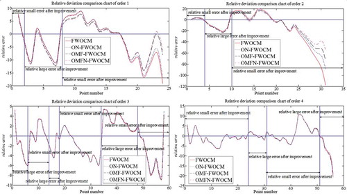
Figure 7. Comparison of the relative deviation of two practical catastrophic flood sequences.

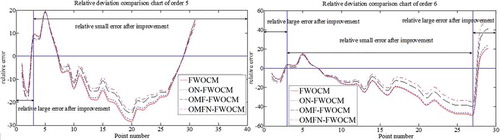
4.2.3 Fitting effect

Analysis of the fitting curves with the points shows that the original method and the improved methods all fit well with the original points, with little difference. The improved methods fit better than the original methods with enhanced tendency and extensibility. For the general flood, the improved methods can obtain larger design values than the original methods. The improved methods can also effectively control the influence of the catastrophic flood to obtain smaller design values than the original method. However, the design values obtained by the improved method need further research and verification.

5 Conclusion

The FWOCM performs better than some other parameter estimation methods such as the optimum curve-fitting method and the ocular estimation because the weights of the points are based on sampling error and are not equal. The weight of the point is able to be calculated by the integral of the membership function in the interval. The deficiency of the integral provided the motivation for this study to improve the FWOCM. The improvement of the method is seen in two advantages: first, the derivation of a more accurate membership function; second, the application of the complete nomograph which covers the whole frequency.

The determination of FWOCM is based on two considerations: (1) there is an ideal curve to a sequence, and (2) the distance of the point to the curve obeys a distribution. Using the two considerations, the improved FWOCMs can be used to estimate the design values of the hydrologic sequences. The improved methods provide each point with a more accurate weight to measure the importance of the point in the curve-fitting method.

In this paper, the statistical unbiasedness and effectiveness of the proposed methods were researched by Monte Carlo statistical tests with the random data that obey the Pearson Type-III distribution. The scoring method and percentage method were proposed to analyse unbiasedness and effectiveness. By comparing the indexes of the improved methods with the original method, this study shows that the improvement of the membership function and nomograph can reduce bias and volatility.

Measured data were also used to test the effectiveness and unbiasedness of the improved FWOCMs. The line charts of the four FWOCMs for the measured data demonstrate that the improved FWOCMs have a better fitting effect than the original method.

Despite these improvements, there are some disadvantages and potential problems that need to be studied. For example, the nomograph of the absolute sum of deviations needs to be extended. The membership function should be developed to adjust the practical data that cannot completely conform to the Pearson-III distribution to improve the fitting effect.

In conclusion, the improved FWOCMs allow accurate estimation of design values for frequency analysis. The optimum curve-fitting effect of the improved methods is satisfactory, and the improved methods are more practical than the original method in engineering application.

Disclosure statement

No potential conflict of interest was reported by the authors.

Additional information

Funding

The authors are grateful for the support of the National Key Research and Development Plan, National Natural Science Foundation of China [No. 51509088; No. U17652010], the “The National Key Research and Development Program of China” [No. 2016YFC0401808], Henan Province University Scientific and Technological Innovation Team [No. 18IRTSTHN009], and Henan Key Laboratory of Water Environment Simulation and Treatment [No. 2017016].

References

- Beven, K. and Binley, A., 1992. The future of distributed models: model calibration and uncertainty prediction. Hydrological Processes, 6 (3), 279–298. doi:10.1002/hyp.3360060305.
- Cao, X., et al., 2010. Application of ant colony algorithm to parameter estimation of P-III type distribution curve. Water Resources and Power, 28 (4), 14–15+74.
- Carroll, R., Wu, C.F.J., and Ruppert, D., 1988. The effect of estimating weights in weighted least squares. Journal of the American Statistical Association, 83 (404), 1045–1054. doi:10.1080/01621459.1988.10478699.
- Chatterjee, S. and Mächler, M., 1997. Robust regression: a weighted least squares approach. Communications in Statistics - Theory and Methods, 26 (6), 1381–1394. doi:10.1080/03610929708831988.
- Chau, K., 2007. A split-step particle swarm optimization algorithm in river stage forecasting. Journal of Hydrology, 346 (3–4), 131–135. doi:10.1016/j.jhydrol.2007.09.004.
- Chen, Y. and Hou, Y., 1992. Research on parameter estimation method for P type-III distribution. Journal of HoHai University, 20 (3), 24–31.
- Chen, Z., et al., 1963. Discussion of Pearson-III curve. Kriczki-Minca curve designing floods. Symposium Science, 2nd set. Beijing: Scientific Research Institute Water Conservancy Hydropower.
- Chen, Z., et al., 2012. Pearson type III distribution parameters estimation based on simulated annealing. Yellow River, 34 (5), 14–15+19.
- Cheng, C., Wu, X., and Chau, K., 2005. Multiple criteria rainfall-runoff model calibration using a parallel genetic algorithm in a cluster of computers. Hydrological Sciences Journal, 50 (6), 1069–1087. doi:10.1623/hysj.2005.50.6.1069.
- Chow, K.C.A. and Watt, W.E., 1994. Practical use of the L-moments. In: K.W. Hipel, ed. Stochastic and statistical methods in hydrology and environmental engineering, Vol. 1. Boston, MA: Kluwer Academic, 55–69.
- Cong, S., Tan, W., and Huang, S., 1980. Statistical testing research on the methods of parameter estimation in hydrological computation. Journal of Hydraulic Engineering, 6 (3), 1–14.
- Cuevas, E., et al., 2013. A swarm optimization algorithm inspired in the behavior of the social-spider. Expert Systems with Applications, 40 (16), 6374–6384. doi:10.1016/j.eswa.2013.05.041.
- Cunnane, C., 1985. Factors affecting choice of distribution for flood series. Hydrological Sciences Journal, 30 (1), 25–36. doi:10.1080/02626668509490969.
- Deng, Y., Ding, J., and Wei, X., 1995. Fuzzy optimum curve fitting method in frequency analysis. Design of Hydroelectric Power Station, 11 (4), 43–47.
- Fotovatikhah, F., et al., 2018. Survey of computational intelligence as basis to big flood management: challenges, research directions and future work. Engineering Applications of Computational Fluid Mechanics, 12 (1), 411–437. doi:10.1080/19942060.2018.1448896.
- Ge, J., 1990. Discussion on hydrologic frequency calculation by Weibull distribution. Yangtze River, (2), 17–25.
- Greenwood, J.A., Landwehr, J.M., and Matalas, N.C., 1979. Probability weighted moment: definition and relation to parameters of several distributions expressible in inverse form. Water Resources Research, 15 (5), 1049–1054. doi:10.1029/WR015i005p01049.
- Guo, S., 1987. Fitting the Pearson type 3 distribution. Journal of Wuhan University of Hydraulic and Electric Engineering, 3, 27–37.
- Haktanir, T., 1997. Self-determined probability-weight moments method and its application to various distributions. Journal of Hydrology, 194, 180–200. doi:10.1016/S0022-1694(96)03206-4
- Haktanir, T. and Horlacher, H., 1993. Evaluation of various distributions for flood frequency analysis. Hydrological Sciences Journal, 38 (1), 15–32. doi:10.1080/02626669309492637.
- Hosking, J.R.M. and Wallis, J.R., 1997. Regional frequency analysis – an approach based on L-Moment. Cambridge, UK: Cambridge University Press, 14–43.
- Jia, P., Li, X., and Wang, J., 2008. The comparison of several kinds of typical comprehensive evaluation methods. Chinese Journal of Hospital Statistics, 15 (4), 351–353.
- Jin, G., 1964. The principles and methods of hydrological statistics. Beijing: China Industrial Press.
- Jin, G., 2001. The discussion for the weight function method of probability distribution parameters. Journal of Hydraulic Engineering, 11 (11), 34–40.
- Jin, G. and Fei, Y., 1991. Determination of the revised coefficient B value in Г distribution. Journal of China Hydrology, 1991 (6), 1–3.
- Karim, M. and Chowdhury, J., 1995. A comparison of four distributions used in flood frequency analysis in Bangladesh. Hydrological Sciences Journal, 40 (1), 55–66. doi:10.1080/02626669509491390.
- Karvanen, J. and Nuutinen, A., 2008. Characterizing the generalized lambda distribution by L-moments. Computational Statistics and Data Analysis, 52 (4), 1971–1983. doi:10.1016/j.csda.2007.06.021.
- Kumar, R., et al., 2003. Development of regional flood frequency relationships using L-moments for Middle Ganga Plains Subzone of India. Water Resources Management, 12 (17), 243–257. doi:10.1023/A:102477012.
- Lei, G., et al., 2015. The application of the TOPSIS-Fuzzy comprehensive evaluation method used in the method of optimizing the hydrologic frequency parameter estimation. Journal of Water Resources Research, 4, 200–207. doi:10.12677/JWRR.2015.42024
- Lei, G., et al., 2018. The analysis and improvement of the fuzzy weighted optimum curve-fitting method of Pearson-Type III distribution. Water Resources Management, 32 (14), 4511–4526. doi:10.1007/s11269-018-2055-9.
- Li, H. and Song, S., 2009. Application of ant colony algorithm in parameter calculation of hydrological frequency curve. Yellow River, 31 (4), 38–40.
- Li, S., 1984. Practicability of several frequency distribution lines for flood data in China. Journal of China Hydrology, 4 (1), 1–7.
- Li, Y. and Song, S., 2014. Application of higher probability weighted moments of P-III distribution to flood frequency analysis. Journal of Hydroelectric Engineering, 33 (3), 10–18.
- Liang, Z., et al., 2014. A modified weighted function method for parameter estimation of Pearson Type Three distribution. Water Resources Research, 50 (4), 3216–3228. doi:10.1002/2013WR013653.
- Liang, Z., Ning, F., and Wang, Q., 2001. Application of weighted function method to hydrological frequency analysis. Journal of HoHai University, 29 (4), 95–98.
- Liu, L., et al., 2009. Application of particle swarm optimization and fitness line method in hydrological frequency analysis. Journal of China Hydrology, 29 (2), 21–23.
- Liu, P., Guo, S., and Hu, A., 2006. Deriving the B nomogram of L-moments method to estimate sampling errors of design floods. Journal of China Hydrology, 26 (6), 27–29.
- MWR (Ministry of Water Resources), 2006. Water resources and hydropower engineering specification design flood calculation. SL44-2006. Beijing, China: Waterpower Press.
- Parida, B.P., Kachroo, R.K., and Shrestha, D.B., 1998. Regional flood frequency analysis of Mahi-Sabarmati Basin (Subzone 3-a) using index flood procedure with L-Moments. Water Resources Management, 12 (1), 1–12. doi:10.1023/A:1007970800408.
- Ponce, V.M., 1989. Engineering Hydrology. Englewood Cliffs, NJ: Pearson, 214–216.
- Qiu, L., Chen, S., and Pan, D., 1998. Weighted optimum curve fitting method for estimating the parameters of Pearson type-III distribution. Journal of Hydraulic Engineering, 29 (1), 33–38.
- Rao, A.R. and Hamed, K.H., 2000. Flood frequency analysis. Boca Raton, FL: CRC Press.
- Sandoval, C. and Villasenor, J., 2008. Trivariate generalized extreme value distribution in flood frequency analysis. Hydrological Sciences Journal, 53 (3), 550–567. doi:10.1623/hysj.53.3.550.
- Sarbu, C., 1995. A comparative study of regression concerning weighted least squares methods. Analytical Letters, 28 (11), 2077–2094. doi:10.1080/00032719508000026.
- Song, M., Feng, P., and Zhang, Z., 2008a. Pearson type-III curve parameter estimation based on Genetic Algorithm. China Rural Water and Hydropower, (6), 52–54.
- Song, S., Kang, Y., and Jing, P., 2008b. Parameter optimum estimation for hydrological frequency curve. Journal of Northwest A&F University (Nat. Sci. Ed), 6 (4), 193–198.
- Song, X. and Ma, X., 2009. Hydrology engineering. Henan: Yellow River Water Conservancy Press.
- Tang, Y., et al., 2015. Application of historical flood-concerned mixed distribution with different tail types of PDFs. Journal of Hydroelectric Engineering, 34 (4), 31–37.
- Taormina, R., Chau, K.-W., and Sivakumar, B., 2015. Neural network river forecasting through baseflow separation and binary-coded swarm optimization. Journal of Hydrology, 529, 1788–1797. doi:10.1016/j.jhydrol.2015.08.008
- Wallis, J.R., et al., 1974. Just a moment! Water Resources Research, 10 (2), 211–219. doi:10.1029/WR010i002p00211.
- Wang, W., et al., 2013. Hydrology engineering. Beijing: China Waterpower Press.
- Wang, W., et al., 2015. The adaptive numerical integral Pearson-III curve parameters estimation based on SSO. Journal of Basic Science and Engineering, S1, 122–133. doi:10.16058/j.issn,1005-0930.2015.s1.013
- Wang, W., et al., 2016. Hydrologic frequency analysis using SSO algorithm. Journal of China Hydrology, 36 (3), 34–39.
- Wang, W., Lei, G., and Liu, K., 2017. Improvement and statistical performance of fuzzy weighted optimum curve-fitting method. Journal of China Hydrology, 37 (5), 1–7.
- Wang, Z., et al., 2009. Application of genetic algorithm in parameter estimation of P type III distribution curve. Yellow River, 31 (9), 21–23.
- Wu, C. and Chau, W., 2011. Rainfall–runoff modeling using artificial neural network coupled with singular spectrum analysis. Journal of Hydrology, 399 (3–4), 394–409. doi:10.1016/j.jhydrol.2011.01.017.
- Wu, G., 2015. Application of social spider optimization algorithm in parameter optimization of hydrological frequency curve. Journal of Water Resources and Water Engineering, 26 (6), 123–126,131. doi:10.11705/j.issn.1672-643X.2015.06.22.
- Xie, C., Yuan, H., and Guo, Y., 1997. A new estimation way of Pearson type-III distribution parameter of frequency curve-fuzzy maximum value method. Journal of China Hydrology, (1), 1–7.
- Xie, P. and Zheng, Z., 2000. A constrained and weighted fitting method for hydrologic frequency calculation. Journal of Wuhan University of Hydraulic and Electrical Engineering, 33 (1), 49–52.
- Yang, R. and Ding, J., 1988. Research on parameter estimation method for P- type III distribution. Journal of Chengdu University of Science and Technology, (2), 37–46.
- Yao, D. and Song, S., 2007. Curve fitting method of design flood frequency based on Particle Swarm Optimization. Bulletin of Soil and Water Conservation, 27 (6), 112–115.
- Ye, Y., 1964. Problem of flood frequency analysis. Assembler of hydrological calculation experience. Beijing: China Industrial Press.
- Ye, Y., et al., 1981. Statistical test research on parameter estimation method in hydrological frequency calculation. Journal of Hydraulic Engineering, 4, 84–90.
- Yu, Y. and He, X., 2012. Maximum likelihood estimation of Pearson-III curve and its application. Yangtze River, 43 (21), 21–23.