Simulation of streamflow with statistically downscaled daily rainfall using a hybrid of wavelet and GAMLSS models

ABSTRACT

A rainfall–streamflow model is proposed, in which a downscaled rainfall series and its wavelet-based decomposed sub-series at optimum lags were used as covariates in GAMLSS (Generalized Additive Model in Location, Scale and Shape). GAMLSS is applied in climate change impact assessment using CMIP5 general climate model to simulate daily streamflow in three sub-catchments of the Onkaparinga catchment, South Australia. The Spearman correlation and Nash-Sutcliffe efficiency between the observed and median simulated streamflow values were high and comparable for both the calibration and validation periods for each sub-catchment. We show that the GAMLSS has the capability to capture non-stationarity in the rainfall–streamflow process. It was also observed that the use of wavelet-based decomposed rainfall sub-series with optimum lags as covariates in the GAMLSS model captures the underlying physics of the rainfall–streamflow process. The development and application of an empirical rainfall–streamflow model that can be used to assess the impact of catchment-scale climate change on streamflow is demonstrated.

KEYWORDS:

• statistical downscaling
• GAMLSS
• rainfall–streamflow
• wavelet transform
• general circulation model

Editor R. Woods Associate editor T. Kjeldsen

1 Introduction

It is important to consider the effects of global climate change and variability in water resource planning and management due to the continuing increase in emissions of greenhouse gases into the atmosphere. Traditionally, in assessment of climate change impact on water availability, hydrological models are calibrated with observed rainfall and then downscaled rainfall from general circulation model (GCM) datasets are introduced to the model for historical simulations and future projections. The major flaw associated with this approach is that the rainfall data used in the model development and application phase are not homogeneous in term of quality, as they originate from different sources with different degree of accuracy. That is why a rainfall–streamflow model will show poor performance in simulating streamflow if the model is calibrated with the observed rainfall and thereafter downscaled rainfall from GCM output datasets is used for streamflow simulation. This type of flaw was identified by Sachindra et al. (2014) and Rashid et al. (2015b) when they assessed this traditional approach and its limitations for downscaling rainfall. Unlike this traditional approach, we calibrate a rainfall–streamflow model with the rainfall downscaled from GCM datasets over a historical period and then introduce future rainfall downscaled from the corresponding GCM into the model to obtain projections of future streamflow.

For projection of future rainfall from GCMs, various downscaling techniques have been proposed and tested by different research groups around the world. For example, parametric and non-parametric regression-based downscaling models have been proposed and applied for downscaling of rainfall (Mehrotra and Sharma 2010, Kannan and Ghosh 2013, Beecham et al. 2014). A recent development in downscaling is the inclusion of nonstationarity, which is important from a climate change perspective (Rashid et al. 2016, Salvi et al. 2016). Downscaling models capable of simulating persistence in daily rainfall time series are suitable to feed into hydrological models for studying climate change impact on water availability. Recent applications of the generalized linear model (GLM) have demonstrated a reasonable performance in reproducing the persistence characteristics of rainfall, such as length and number of consecutive dry and wet spells (Pulquério et al. 2015, Rashid et al. 2015b, 2017).

While physically based and conceptual hydrological model need large datasets, empirical models can be fitted by only rainfall data to simulate streamflow. One of the challenges in using physically based and/or conceptual hydrological models for catchment-scale studies of climate change impact is that various climate variables, such as temperature, evapotranspiration and soil moisture, need to be downscaled before being used in models for streamflow simulation. This is both time-consuming, costly and makes the model outputs more uncertain due to the increased number of parameters required, compared to empirically based hydrological models. Additionally, in many cases empirical models outperform conceptual hydrological models; for example, Nayak et al. (2013) showed that a wavelet-based artificial neural network (WANN) model performs better than a conceptual hydrological model (in this case MIKE11-NAM) in estimating the hydrograph characteristics such as the flow duration curve. While several empirical hydrological models have been proposed in previous studies (Wang et al. 2008, Nourani et al. 2011, Kamruzzaman et al. 2013, Kisi et al. 2013, Modarres and Ouarda 2013, Farajzadeh et al. 2014), application of these models for assessing climate change impacts on water resources is limited. Therefore, the development of a parsimonious rainfall–streamflow model for climate change impact studies is important.

The rainfall–streamflow process is a highly complex, non-linear and non-stationary phenomenon in the hydrological cycle. The Generalized Additive Model in Location, Scale and Shape (GAMLSS), proposed by Rigby and Stasinopoulos (2005), provides a flexible framework for non-linear and non-stationary modelling. The dependence of the distribution parameters on covariates can be represented in terms of linear or nonlinear, parametric and/or additive nonparametric functions. GAMLSS has been used successfully to model different hydro-climatic variables, such as rainfall, temperature, flood peaks and streamflow (Villarini et al. 2009, 2010, Van Ogtrop et al. 2011, Villarini and Serinaldi 2012, López and Francés 2013, Rashid et al. 2015a). Addressing nonstationarity in the rainfall–streamflow process is a challenging task and is vital for the study of climate change impact on future water availability.

The wavelet transform (WT) can handle non-stationary signals by decomposing into sub-signals at different temporal scales (levels) and is helpful in better interpreting hydrological processes (Kisi and Cimen 2012, Rashid et al. 2016, 2018). Lower-level-decomposed sub-series contain high-frequency components (rapidly changing events) and higher-level-decomposed sub-series represent the low-frequency components (slowly changing events) of the original signal. Anctil and Tape (2004) combined wavelet decomposition and ANNs to forecast next-day streamflow from rainfall and potential evapotranspiration time series. Nourani et al. (2009) claimed that extraction of multi-scale characteristics of the time series is helpful to predict short- and long-term runoff when a coupled wavelet-ANN model (WANN) is used to simulate the rainfall–runoff process.

The main objective of this research is to develop a novel rainfall–streamflow model in which a daily rainfall series downscaled from NCEP reanalysis and GCM datasets is used as model input to simulate daily streamflow, and the model performance is assessed against historical-observed streamflow. The modelling is carried out for three sub-catchments of the Onkaparinga catchment in South Australia (SA). In this approach, the downscaled rainfall series and its wavelet-based decomposed sub-series at optimum lags are used as covariates, and the GAMLSS is used as a model engine. The focus of this paper is on the rainfall–streamflow modelling; a related paper by Rashid et al. (2015b) describes the downscaling method and discusses in detail the verification of rainfall simulations against historical-observed rainfall data. The key innovations of this study include the following: (1) unlike traditional approaches, the presented rainfall–streamflow model is calibrated and driven by downscaled rainfall to maintain homogeneity of the predictor data; (2) wavelet-filtered rainfall at different frequency bands is used to capture the potential influence of the low-frequency variability of rainfall on a slowly evolving rainfall–streamflow relationship; (3) GAMLSS is used to model nonlinear rainfall–streamflow relationships; and (4) a zero-adjusted gamma distribution is used to model the occurrence and amount of daily streamflow simultaneously instead of using two separate models.

2 Study area and data

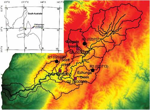
The study area is the Onkaparinga catchment in South Australia. Three sub-catchments, namely Scott Creek, Echunga Creek and Aldgate Creek, are considered for the case study. These were selected as they are the prime contributors of inflow to the main supply reservoir for Adelaide (Mount Bold). The streamflow and rainfall stations are shown in Fig. 1 and details are presented in Table 1. Daily streamflow data were collected from the Bureau of Meteorology (BOM), Australia. In order to obtain an unbroken continuous record among the three selected streamflow stations, daily streamflow data from 1973–2000 were considered in this study. The SILO database of the Queensland Climate Change Centre of Excellence¹ was considered for observed daily rainfall for the period 1961–2000. The atmospheric predictor data (NCEP reanalysis data of the National Centers for Environmental Predition/National Center for Atmospheric Research) for the period 1961–2000 were collected from the National Oceanic and Atmospheric Administration/Earth System Research Laboratory (NOAA/ESRL). To downscale GCM outputs to daily rainfall, the second-generation Canadian Earth System Model GCM (CanESM2) of the Coupled Model Intercomparison Project Phase 5 (CMIP5) was considered in this study. To keep consistency between NCEP and GCM resolution, the GCM outputs were linearly interpolated. Twelve grid points were considered around the study area to extract NCEP reanalysis and GCM data (see Fig. 1).

Table 1. Rainfall and streamflow stations for each sub-catchment considered in the study. Australian Bureau of Meteorology station numbers are given in parentheses.

Catchment	Sub-catchment	Rainfall station	Streamflow station
Onkaparinga	Scott Creek	R1 (023709)	Q1 (5030502)
	Echunga Creek	R2 (023713)	Q2 (5030506)
	Aldgate Creek	R3 (023707)	Q3 (5030509)

Figure 1. Study area and locations of the sub-catchments and rainfall and streamflow stations.

3 Methodology

3.1 Rainfall–streamflow model formulation

South Australia has significant seasonal variability in its streamflow data, because of its winter dominating rainfall (Rashid et al. 2014b). Therefore, in the winter season (June–August), positive streamflow values are often recorded, whereas little or no streamflow is generally recorded in summer (December–February). So, two different models – occurrence and amount – are generally used: an occurrence model to identify a day with non-zero flow and an amount model to estimate the amount of streamflow (Van Ogtrop et al. 2011). In this study, instead of using two different models, a mixed distribution, referred to as a zero-adjusted gamma (ZAGA) distribution, was fitted to the observed daily streamflow. The ZAGA is a special type of zero-adjusted distribution that is appropriate to use when the response variable Y_i (in our case, daily streamflow) contains values from zero to infinity including zero, i.e. [0, ∞]. The ZAGA is a mixture of discrete 0 values with probability${\theta }_3$ and a gamma distribution $\mathrm{G}\mathrm{A}\left({\theta }_1,{\theta }_2\right)$ with probability $(1-{\theta }_3)$. The probability density function of $\mathrm{Z}\mathrm{A}\mathrm{G}\mathrm{A}\left({\theta }_1,{\theta }_2,{\theta }_3\right)$ is given by:

(1) $f_Y\left(y|{\theta }_{1,}{\theta }_2,{\theta }_3\right)=\left\{\begin{array}{c}{\theta }_{3}ify=0\\ \left(1-{\theta }_3\right)f_w\left(y|{\theta }_1,{\theta }_2\right)ify>0\end{array}\right.$(1)

for $0\le y\le \mathrm{\infty }$, where ${\theta }_1>0$ and ${\theta }_2>0$ and $0<{\theta }_3<1$, and $W\sim \mathrm{G}\mathrm{A}\left({\theta }_1,{\theta }_2\right)$ has a gamma distribution.

The GAMLSS was used for rainfall–streamflow modelling. Details of the GAMLSS are available in Rigby and Stasinopoulos (2005) and Stasinopoulos and Rigby (2007). A semi-parametric additive model formulation was considered in this study as:

(2) $g_k\left({\mathit{\theta }}_k\right)={\mathit{X}}_k{\mathit{\beta }}_k+{\sum }_{j=1}^{j_k}{h}_{jk}\left(x_{jk}\right)$(2)

where θ^k is a vector that represents the parameters of the distribution, X_k is a matrix of covariates of order n × j_k, β(β_1k, …, β_j,k) is a parameter vector of length j_k, and $h_{jk}(.)$ represents the dependence function of the distribution parameters on the covariates. The dependence could be linear or a smoothing term can be included to allow more flexibility for modelling the dependence of the distribution parameters on the covariates.

3.2 Rainfall downscaling model

In this study, the rainfall–streamflow model is calibrated with downscaled rainfall instead of observed rainfall to keep homogeneity in the predictor data for the development and application phases of the model, as discussed earlier. The Generalized LInear Modelling of daily CLImate sequence (GLIMCLIM) (Chandler 2002) is a multi-site stochastic downscaling model, based on a generalized linear model (GLM), which is used to downscale daily rainfall from reanalysis and GCM output datasets. Details of this downscaling methodology are reported in Beecham et al. (2014) and Rashid et al. (2015b). A short description of the downscaling model is provided here. The GLM-based modelling framework is used for incorporating climate predictors in the downscaling model. For a n× 1 vector of a random variable (i.e. rainfall) Y =(Y₁, …, Y_n), each dependent on predictors p (n × p matrix), a probability distribution of Y can be specified with a vector of mean μ =(μ₁, …, μ_n) by:

(3) $g(\mu )=X\mathit{\beta }$(3)

where g(.) is a monotonic or link function and β is a vector of coefficients. A two-step modelling approach is adopted, in which the occurrence of daily rainfall is modelled with a logistic regression, and the rainfall amounts in wet days are estimated from a gamma distribution fitted to the observed wet day rainfall conditioned to predictor variables. Simulated rainfall outputs from the GLIMCLIM model over the period 1973–2000 are considered for calibration and validation of the rainfall–streamflow model.

3.3 Predictors of the rainfall–streamflow model

There are different wavelet functions, such as the Haar wavelet (Haar 1910), the Daubechies wavelet (Daubechies 1988), the Mexican Hat wavelet (normalized second derivative of the Gaussian function) and the Morlet wavelet (Morlet et al. 1982). Among these, the Haar wavelet is conceptually simple, computationally fast and exactly reversible. In this study, the discrete wavelet transform (DWT) is performed using the widely applied Harr wavelet. Eight resolution levels are considered to decompose the time series. For a sampling period of one day and resolution levels of $j=$ 1, 2, 3, 4, 5, 6, 7 and 8, the time scales of the wavelet decomposition are 2, 4, 8, 16, 32, 64, 128 and 256 days, respectively. The time series is decomposed into one that represents the trend, termed the approximation (A), and one that represents the frequently occurring events, termed the details (D). For a detailed theory of wavelet transform, readers are referred to Torrence and Compo (1998). Thus, the downscaled rainfall series is decomposed into eight levels using DWT and nine decomposed sub-series, D1–D8 and A8 are obtained (see Section 4.2). In modelling streamflow, we assume that the original and decomposed rainfall sub-series have influence on the observed streamflow with some time lag. A cross-correlation analysis is implemented to identify the lag relationships. The lag correlation coefficient between two series is used for this purpose. When maximum lag correlation at the 95% confidence level is identified, the corresponding lag series of the decomposed rainfall sub-series is used as potential covariate for streamflow modelling. In the case of the original rainfall series, up to 3 days’ previous rainfall in addition to the present-day rainfall are considered as potential covariates. In addition, the sinusoidal terms $C=\mathrm{c}\mathrm{o}\mathrm{s}\left(\frac{2\pi t}{365.25}\right)$ and $S=\mathrm{s}\mathrm{i}\mathrm{n}\left(\frac{2\pi t}{365.25}\right)$ are used to allow for seasonal variations.

3.4 Lag time estimates

Lag correlation refers to the correlation between two time series shifted in time in relation to one another. Cross-correlation is an effective method to assess the lag relationship between two time series. The optimum lag time is estimated by finding some previous time at which the cross-correlation is maximum. In this study, downscaled daily rainfall series are decomposed into nine sub-series, and a cross-correlation analysis is implemented to identify the lag relationships between the rainfall sub-series and the observed streamflow. If $x_i$ and $y_i$ are two time series, with i= 1, 2, 3, …, N, the cross-correlation coefficient r at any lag k is defined by:

(4) $r\left(k\right)=\frac{{\sum }_{i=1}^N\left[x\left(i\right)-\bar{x}\right][y\left(i-k\right)-\overline{y]}}{\sqrt{{\sum }_{i=1}^N{\left[x\left(i\right)-\bar{x}\right]}^2{\sum }_{i=1}^N[y\left(i-k\right)-{\overline{y]}}^2}}$(4)

where $\bar{x}$ and $\bar{y}$ are the mean of the $x_i$and $y_i$time series, respectively. The optimal lag time between two time series is obtained from the maximum of$r\left(k\right)$ at the 95% significance level. In this way, lag times are identified for each potential predictor for streamflow modelling. This method of finding optimal lag time and using time series of that lag directly in the model is useful and less time-consuming than including time series of different lags in the model for finding the significant lag series.

3.5 Fitting of the rainfall–streamflow model

The stepwise model-fitting approach proposed by Rigby and Stasinopoulos (2005) is followed to identify the significant covariates for each distribution parameter. The Akaike information criterion (AIC) and Schwarz Bayesian information criterion (SBIC) are used for the selection of significant covariates. In addition, the normality and independence of the residuals are assessed by examining the first four moments of the residuals, the Filliben correlation coefficient (Filliben 1975) and by visual inspection of a diagnostic plot of the residuals including qq and worm plots. The model is calibrated in the period 1973–1990 and validated in the period 1991–2000. Then, the model is used to simulate the streamflow for the future period 2041–2060 using the downscaled rainfall and its wavelet-based decomposed sub-series at optimum lags as covariates. For each period, 100 sets of synthetic streamflow series are generated.

4 Results

4.1 Downscaled rainfall

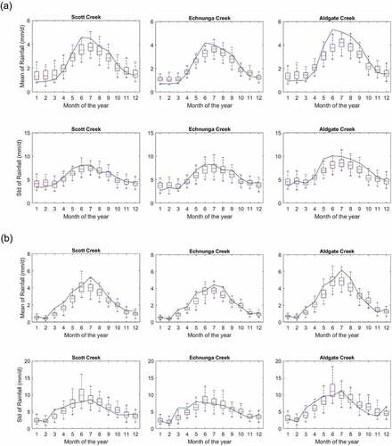
The GLIMCLIM model was used to downscale multi-site daily rainfall from NCEP reanalysis datasets. Statistical downscaling often assumes that the relationship between predictors and predictands is stationary and remains unaltered, but this is not necessarily valid in a changed climate. A design-of-experiments (DOE) strategy, proposed by Salvi et al. (2016), was employed to assess the performance of the downscaling model under a nonstationary climate. Two different tests were performed: the downscaling model was calibrated and validated (a) on the periods 1961–1986 and 1987–2000, respectively; and (b) on the periods 1991–2010 and 1981–1990, respectively. For the former case, the calibration and validation periods were comparatively wet and dry, respectively, and for the latter, the periods were comparatively dry and wet, respectively (Beecham et al. 2014). Figure 2 shows the mean and standard deviation of the observed and simulated daily rainfall for different months of the year at three rainfall stations corresponding to the selected sub-catchments (Table 1) for both cases (a) and (b). The results presented in Fig. 2 show that the downscaling model was able to reproduce the mean and standard deviation of the observed rainfall for each month of the year with a good degree of accuracy for all three rainfall stations. However, the model shows a tendency to overestimate for summer (December–February) and underestimate for winter (June–August) for case (a), although the observations are within the simulation envelope. Therefore, the GLM-based downscaling model is capable of performing reasonably well even under a nonstationary climatic condition.

Figure 2. Mean and standard deviation of observed and simulated rainfall for different months of the year at three rainfall stations: from left to right, R1, R2 and R3, corresponding to the three study sub-catchments, for the validation periods (a) 1987–2000 and (b) 1981–2000. Solid curves represent the observations, while the box plots show the range of median and inter-quartile range (IQR) values for 1000 simulations. The whiskers represent 1.5 IQR from the box end.

4.2 Lag relation between streamflow and decomposed rainfall sub-series

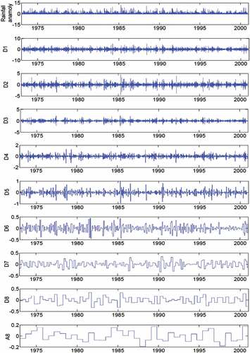
Figure 3 shows the discrete wavelet decomposition of the daily rainfall series for the Scott Creek sub-catchment (Station R1). This shows the original rainfall anomaly and its details (D1–D8) and approximation (A8) sub-series. Table 2 lists the lags (in days) at which maximum correlations are observed for different decomposed rainfall sub-series with corresponding streamflow for three sub-catchments. It is clear that the lag of maximum correlation for any decomposed sub-series may be different for different streamflow series pertaining to different sub-catchments. This depends on the catchment characteristics, such as soil type, infiltration capacity, vegetation type, catchment slope and land use. It was found that decomposed sub-series at higher levels provide significant lag relationships, whereas those at lower levels do not show any significant lag relationship. This is due to the fact that the higher-level-decomposed sub-series are slowly varying with higher periodic components of rainfall that cause a delayed response in the streamflow. Moreover, high-level-decomposed rainfall sub-series (D6–D8 and A8) are significantly correlated with climate indices, such as Niño3.4 (not shown here), which demonstrates that these sub-series are a surrogate of climate indices and are useful for capturing the low-frequency variability of streamflow. The association of Australian rainfall with different climate indices has already been identified in previous studies (Speer et al. 2011, He and Guan 2013, Rashid et al. 2014a).

Table 2. Lags of statistically significant (at the 95% significance level) maximum correlation between decomposed rainfall sub-series and streamflow for three sub-catchments.

Rainfall sub series	Lag (days) of maximum correlation
	Scott Creek	Echunga Creek	Aldgate Creek
D1	0	0	0
D2	0	0	0
D3	0	0	0
D4	0	1	0
D5	0	0	0
D6	11	5	5
D7	2	20	19
D8	23	22	20
A8	11	11	14

Figure 3. Decomposed sub-series (details, D1–D8 and approximation, A8) of the standardized rainfall series at rainfall station R1.

4.3 Covariate analysis

The GAMLSS model was fitted separately to each observed streamflow series for three sub-catchments over the calibration period 1973–1990. The time series of optimum lags obtained from different decomposed rainfall sub-series were considered as potential covariates for streamflow modelling. In the case of the original rainfall series, present-day and up to 3 days of previous rainfall were considered as potential covariates. Table 3 summarizes the significant covariates for all parameters of the distribution for each sub-catchment.

Table 3. Summary of fitted models for each sub-catchment with significant covariates for different parameters of the distribution.

Sub-catchment	Streamflow station ID	Distribution parameters	Significant covariates*
Scott Creek	5030502	${\theta }_1$	cs(R) + R1 + R2 + R3 + S + C + A811 + D1+ D2 + cs(D3) + D4 + cs(D72) + cs (D823) + D72:D823
		${\theta }_2$	cs(R) + cs(S) + cs(C) + cs(D3) + cs(D72) + cs(D823) + D72:D82
		${\theta }_3$	cs(D72) + S + cs(C) + cs(D823)
Echunga Creek	5030506	${\theta }_1$	cs(R) + cs(R1) + cs(R3) + cs(S) + cs(C) + A811 + cs(D5) + cs(D65) + cs(D720) + cs (D822) + D720:D823
		${\theta }_2$	cs(R) + cs(R3) + cs(S) + cs(C) + cs(D5) + cs(D65) + cs(D720) + D720:D823
		${\theta }_3$	cs(R) + cs(R3) + cs(S) + cs(C) + cs(D65) + cs(D720) + cs(D822) + D720:D823
Aldgate Creek	5030509	${\theta }_1$	cs(R) + cs(S) + cs(C) + cs(A814) + cs(D5) + cs(D65) + cs(D719) + cs(D820) + rlag1:S
		${\theta }_2$	cs(S) + cs(C) + cs(A814) + cs(D5) + cs(D65) +cs(D719) + cs(D820)
		${\theta }_3$	cs(C) + cs(D5) + cs(D65) + cs(D719) + cs(D820)

*R is the original rainfall series and R₁, R₂ and R₃ are the 1-, 2- and 3-day lag rainfall series, respectively. S and C are the sine and cosine terms. D1, D2, …, D8 are different decomposed rainfall sub-series without lag. Decomposed rainfall series with lag are represented by the lag number as a subscript, for example, decomposed series D2 with a lag of 5 days is given by D2₅.

4.4 Calibration and validation results

The performance statistics of the model used to simulate daily streamflow for the calibration and validation periods are presented in Table 4. The performance statistics were estimated based on the observed and median simulated streamflow. It was observed that the model was able to reproduce the observed daily streamflow for each sub-catchment. Both the average and standard deviation of the observed streamflow were reasonably simulated by the model (Table 4). Spearman correlations among the observed and median simulated streamflow were high and comparable for both the calibration and validation periods for each sub-catchment. In terms of average and standard deviation of simulated rainfall, the best performance of the model is observed for the Aldgate Creek sub-catchment. The observed mean streamflow of 7.24 and 6.14ML/d for the calibration and validation periods were reproduced by the model as 7.19 and 6.73ML/d, respectively. The model for the Aldgate Creek sub-catchment yielded Spearman correlation coefficients of 0.72 and 0.69 in the calibration and validation periods, respectively.

Table 4. Comparison between the observed and median simulated daily streamflow for three sub-catchments over the calibration and validation periods. Avg: average streamflow (ML/d); SD: standard deviation of streamflow (ML/d); Max: maximum streamflow (ML/d); MB: mean bias; Scorr: Spearman correlation.

	Calibration period, (1973–1990)		Validation period, (1991–2000)
Statistics	Observed	Simulated	Observed	Simulated
Scott Creek
Avg	9.85	9.70	10.82	9.71
SD	29.71	24.80	33.02	28.17
Max	675.30	640.71	624.81	755.77
MB	N/A	0.15	N/A	1.11
Scorr	N/A	0.73	N/A	0.72
Echunga Creek
Avg	9.56	8.54	9.86	7.35
SD	37.01	40.93	46.09	33.05
Max	989.80	1449.61	1070.28	924.54
MB	N/A	1.01	N/A	2.51
Scorr	N/A	0.78	N/A	0.74
Aldgate Creek
Avg	7.24	7.19	6.14	6.73
SD	17.02	14.77	12.91	14.06
Max	363.97	270.23	208.00	250.80
MB	N/A	0.05	N/A	−0.59
Scorr	N/A	0.72	N/A	0.69

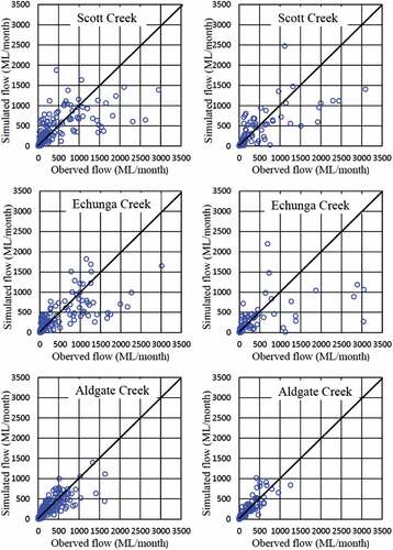
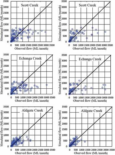
Model performance was also evaluated by comparing the observed and median simulated monthly streamflow in terms of the mean, standard deviation, correlation coefficient, Nash-Sutcliffe efficiency criterion and a scatterplot. Figure 4 shows the scatterplot of observed and median simulated monthly streamflow for the calibration and validation periods. In the case of the Scott Creek and Echunga Creek sub-catchments, lower streamflow was slightly over-predicted, and higher streamflow was under-predicted for both the calibration and validation periods. However, a low scatter revealed that the model reproduced the monthly total rainfall in the Aldgate Creek sub-catchment with higher efficiency compared to the other two sub-catchments.

Figure 4. Scatterplots of observed and median simulated monthly streamflow for the calibration (left) and validation (right) periods.

Table 5 lists the performance statistics of the model used to simulate the monthly streamflow in the three sub-catchments for the calibration and validation periods. In the calibration period, observed average streamflow of 298.78 and 219.55ML/month at Scott Creek and Aldgate Creek, respectively, was reproduced by the model as 294.26 and 218.08ML/month, respectively. The average streamflow at Echunga Creek was under-predicted by the model in the calibration period. The standard deviation of the observed streamflow was under-predicted by the model for all sub-catchments for both the calibration and validation periods. The coefficient of variation (CV) of the observed streamflow over the calibration and validation periods was almost the same for the Scott Creek and Aldgate Creek sub-catchments, and the model reproduced these CV values reasonably well. The observed streamflow data for the Echunga Creek sub-catchment had a larger scatter in the validation period (CV = 2.24) compared to the calibration period (CV = 1.92). The observed CV for the calibration period was exactly reproduced by the model as CV = 1.92, while it was under-estimated as 1.88 for the validation period. For the calibration period, Nash-Sutcliffe efficiency (NSE) statistics of 0.49, 0.67 and 0.66 were observed for the Scott Creek, Echunga Creek and Aldgate Creek sub-catchments, respectively, compared to NSE of 0.54, 0.41 and 0.70, respectively, for the validation period. The model provided a slightly better fit for the validation period in terms of there being fewer outliers for this period.

Table 5. Comparison between the observed and median simulated monthly streamflow for three sub-catchments over the calibration and validation periods. Avg: average of streamflow (ML/month); SD: standard deviation of steamflow (ML/month); CV: coefficient of variation; R²: coefficient of determination; NSE: Nash-Sutcliffe efficiency criterion.

	Calibration period, (1973–1990)		Validation period, (1991–2000)
Statistics	Observed	Simulated	Observed	Simulated
Scott Creek
Avg	298.78	294.26	329.32	295.49
SD	502.30	388.59	557.06	430.28
CV	1.68	1.32	1.69	1.46
R^2	N/A	0.49	N/A	0.55
NSE	N/A	0.49	N/A	0.54
Echunga Creek
Avg	289.90	259.17	300.04	223.67
SD	557.85	498.14	672.43	419.40
CV	1.92	1.92	2.24	1.88
R^2	N/A	0.68	N/A	0.44
NSE	N/A	0.67	N/A	0.41
Aldgate Creek
Avg	219.55	218.08	186.89	204.88
SD	291.09	254.82	228.25	242.00
CV	1.33	1.17	1.22	1.18
R^2	N/A	0.66	N/A	0.73
NSE	N/A	0.66	N/A	0.70

Although almost the same mean monthly rainfall was observed in the Scott Creek and Aldgate Creek sub-catchments (Fig. 2), the observed mean monthly streamflow in the Aldgate Creek sub-catchment was significantly lower than that in the Scott Creek sub-catchment for both the calibration and validation periods. This difference in streamflow will have occurred due to the difference in catchment characteristics, such as soil type, vegetation type, catchment slope and land use. Due to such differences, the direct contribution of rainfall to streamflow in the Aldgate Creek sub-catchment might be less than that in the Scott Creek sub-catchment, which would explain the differences in streamflow between the two sub-catchments. Nevertheless, the hybrid wavelet-GAMLSS model was able to reproduce the observed streamflow statistics with a good degree of accuracy for both sub-catchments, as shown in Table 5. This is due to the fact that wavelet decomposed rainfall sub-series at optimum lag were used as covariates in the model. While the original rainfall series (present-day and up to 3 days’ previous rainfall) used in this study represent mostly the direct contribution to streamflow, high-level (low-frequency) decomposed rainfall sub-series represent the contribution from the rainfall that is stored in the landscape depressions and infiltrated into the soil. It may be observed in Table 3 that the original rainfall series (except present-day rainfall for parameter θ₁) was not significant in the rainfall–streamflow model for the Aldgate Creek sub-catchment. However, decomposed rainfall sub-series at high level were significant for all three distribution parameters (θ₁, θ₂ and θ₃). This implies that the streamflow in the Aldgate sub-catchment is characterized by the low-frequency variability of rainfall, which conceptually represents the contribution to streamflow from the rainfall that infiltrates into the soil. Therefore, this study demonstrates that using a wavelet decomposed sub-series at optimum lags as covariate in the GAMLSS model is useful for capturing the underlying physics of the rainfall–streamflow process.

Figure 5 shows the flow duration curves (FDC) of the observed and simulated streamflow for the three sub-catchments in the calibration and validation periods. In the case of Scott Creek and Echunga Creek, the model was able to reasonably reproduce the observed FDCs for both the calibration and validation periods; however, the Echunga Creek low flows (lower than the 8th percentile of flow) were consistently underestimated by the model in the validation period. For the Aldgate Creek sub-catchment, the FDC of the observed streamflow for the calibration period (1973–1990) shows that there was at least some streamflow over the period, whereas the FDC of the observed streamflow for the validation period (1991–2000) shows that there was a complete absence of streamflow for almost 11% of the days (Fig. 5). This could be referred to as a flow regime change in the Aldgate Creek sub-catchment. FDCs produced from the simulated streamflow for the validation period show that there was a complete absence of streamflow for almost 5% of days because the model over-estimated the occurrence of non-zero flows. While the proposed model was able to pick up this flow regime change, it was not sufficiently accurate for exact reproduction. This might be due to the fact that the model proposed in this study does not consider changes in catchment response to streamflow due to land-use change and subsequent alteration of streamflow by infrastructure such as farm dams.

Figure 5. Flow duration curves (FDC) of daily streamflow for the Scott Creek, Echunga Creek and Aldgate Creek sub-catchments. Blue and red curves represent the FDCs of the observed streamflow in the calibration (1973–1990) and validation (1991–2000) periods, respectively; grey curves represent the FDCs for individual simulations.

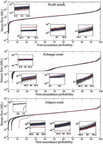
The median simulated daily low flows (10th percentile flows) were underestimated in relation to the observed flows by 12% (Scott Creek), 1.3% (Echunga Creek) and 1.8% (Aldgate Creek) for the calibration period. However, for the validation period, the median simulated low flows were overestimated by 18.0% (Scott Creek) and underestimated by 2.9% (Echunga Creek). In the case of the 50th percentile flows, median-simulated flows were overestimated by 0.3% (Scott Creek) and 7.1% (Aldgate Creek) and underestimated by 13.4% (Echunga Creek) for the calibration period. For the validation period, these were overestimated by 3.9% (Echunga Creek) and 14.4% (Aldgate Creek) and underestimated by 40.8% (Scott Creek). The 95th percentiles of daily flows were overestimated by 7.1% (Scott Creek) and 8.3% (Aldgate Creek) and underestimated by 13.7% (Echunga Creek) for the calibration period. For the validation period, these flows were underestimated by 5.1% (Scott Creek) and 28.8% (Echunga Creek) and overestimated by 31.3% (Aldgate Creek). High flows (99th percentile flows) were underestimated by 37.2% (Scott Creek), 19.2% (Echunga Creek) and 23.0% (Aldgate Creek) for the calibration period, while for the validation period high flows were underestimated by 46.3% (Scott Creek) and 11.1% (Echunga Creek) and overestimated by 7.7% (Aldgate Creek).

4.5 Application for climate change impact assessment

To examine the applicability of the proposed hybrid model for the assessment of climate change impact on streamflow, a rainfall–streamflow model was also developed using downscaled historical rainfall from CMIP5 GCM outputs. The model was then used to simulate future streamflow using downscaled rainfall over the future period 2041–2060. The CanESM2 GCM was considered for this purpose. In this case, the model was calibrated in the period 1973–1990 and validated in the period 1991–2000. Significant covariates of the rainfall–streamflow model developed with rainfall downscaled from NCEP reanalysis (referred to as R_NCEP) were used for the model developed with rainfall downscaled from the CanESM2 GCM outputs (referred to as R_CAN). This means that the model developed with historical R_CAN and R_NCEP rainfall had the same covariates but different optimum values (constants and coefficients in the GAMLSS equations).

This study shows that the model developed with R_CAN was able to reasonably reproduce the historical monthly streamflow for the sub-catchments. Nash-Sutcliffe efficiency statistics of 0.46, 0.40 and 0.55 were obtained for the Scott Creek, Echunga Creek and Aldgate Creek sub-catchments, respectively, for the calibration period compared to NSE values of 0.44, 0.26 and 0.50, respectively, for the validation period. Figure 6 shows the scatterplot of observed and median simulated monthly streamflow for the calibration and validation periods. Like the model developed with R_NCEP, the model developed with R_CAN shows that there is a tendency to underestimate the higher streamflow in the Scott Creek and Echunga Creek sub-catchments.

Figure 6. Scatterplots of observed and median simulated monthly streamflow for the calibration (left) and validation (right) periods using the model developed with historical R_CAN.

The rainfall–streamflow model developed with historical R_CAN (1973–1990) data was used to simulate future streamflow over the period 2041–2060 for the three sub-catchments, driven by R_CAN for the future period. Figure 7 shows the projected changes in monthly streamflow for the period 2041–2060 compared to the reference period of 1973–2000 for the CanESM2 GCM under the (representative concentration pathway) scenario RCP4.5. The results suggest that there will be a significant reduction of streamflow in all three sub-catchments. Westra et al. (2015) also reported that streamflow in the Scott Creek, Echunga Creek and Houlgrave Weir sub-catchments may be reduced in the future. This was the result of simulated future streamflow obtained by feeding downscaled hydro-meteorological variables (rainfall and evapotranspiration) into the conceptual hydrological model GR4J (modèle du génie rural à 4 paramètres journalier).

Figure 7. Projected changes (%) in streamflow for the CanESM2 GCM under the RCP4.5 scenario for the period 2041–2060 compared to the reference period 1973–2000. The boxplots depict the range of median and inter-quartile range (IQR) values for each model for 100 simulations; the whiskers represent 1.5 IQR from the box end.

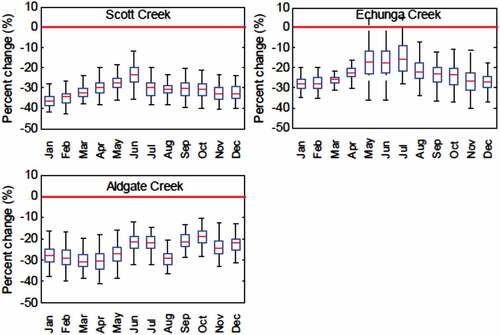
In general, a higher reduction of streamflow is projected to occur in summer (DJF) and spring (SON), while the reduction of streamflow in winter (JJA) will be relatively lower. This pattern of future reduction in streamflow is consistent with the pattern of future reduction in rainfall reported by Rashid et al. (2015b) for the same catchment. They projected that the reduction in summer and spring rainfall will be higher than for winter rainfall. This indicates that the rainfall–streamflow model developed in this study is able to capture the dynamic relationship between rainfall and streamflow and is able to successfully project future changes in streamflow.

Streamflow reduction in the winter season is hydrologically important in the hydrology of this region because the rainfall in the study area occurs predominantly in the winter, and even a small percentage change will cause a large reduction in the total amount of water available in a given year. Historical observations show that the selected sub-catchments have low or no flow during summer. Therefore, it will be particularly challenging in the future to maintain environmental flows through these creeks due to the projected reduction in summer streamflow. This research indicates that South Australian water resource planners need to consider the possibility of significant drier flow regimes in the future when planning for sustainable management of water resources. Due to the possibility of future water shortages, careful evaluation is needed for future water allocations between the three main consumers, water supply for Adelaide, irrigation water for farms and water requirements for maintaining environmental flows in these three sub-catchments.

It should be noted that for these three sub-catchments, the future changes in streamflow projected in this study do not account for the full range of climate change impacts because these are based on one GCM and one scenario (RCP4.5). The intention was to demonstrate the application of the proposed rainfall–streamflow model to assess the climate change impact on streamflow. However, the methodology developed in this study can be applied to assess future changes of streamflow for other GCMs and scenarios. The objective of this study was to develop an empirical rainfall–streamflow model in which streamflow can be simulated with only downscaled rainfall. While evapotranspiration is one of the important inputs for streamflow simulations, particularly when climate change is concerned, this study demonstrates that the model developed was able to reproduce streamflow in the historical period. Moreover, the projection of future changes in streamflow is also consistent with other studies that used conceptual hydrological models, for example Westra et al. (2015) In addition, the decomposed rainfall sub-series at the low frequencies used in the model represent the contribution to streamflow from the rainfall that infiltrates into the soil and this acts as a surrogate for evapotranspiration and infiltration processes. However, the model proposed herein is not a substitute for conceptual hydrological models; rather, it provides an alternative relatively simple, quick and cost-effective option for assessment of climate change impact on future water availability. This empirical model can be particularly useful for situations where hydrological data are restricted to rainfall and streamflow.

5 Conclusion

In catchment-scale climate change impact studies on water resources, hydrological models are often applied to simulate future streamflow projections using downscaled hydro-climatic variables such as rainfall, temperature and evapotranspiration. While physically based and conceptual hydrological models require several downscaled variables for estimating runoff, an empirical rainfall–streamflow model can provide a suitable alternative approach in which only downscaled rainfall data are required for simulating streamflow, thereby reducing the computational cost, complexity and uncertainty. In this study, a rainfall–streamflow model was developed in which the original series of downscaled rainfall and its wavelet-based decomposed sub-series were used as covariates to develop a GAMLSS model to simulate streamflow in three sub-catchments of the Onkaparinga catchment in South Austalia.

A GAMLSS model was fitted to observed streamflow series in three sub-catchments for a calibration period (1973–1990) and a validation period (1991–2000). The model was able to reproduce the observed mean and standard deviation of daily streamflow with a good degree of accuracy for each sub-catchment. Spearman correlations among the observed and median simulated streamflow in each sub-catchment were high and comparable for both the calibration and validation periods. The Nash-Sutcliffe efficiency (NSE) statistics between the median simulated and observed monthly streamflow were 0.49, 0.67 and 0.66 for the Scott Creek, Echunga Creek and Aldgate Creek sub-catchments, respectively, for the calibration period and 0.54, 0.41 and 0.70, respectively, for the validation period. This study shows that the maximum lag correlation between decomposed rainfall sub-series and streamflow varies among the sub-catchments due to the difference in rainfall–streamflow processes that are highly dependent on soil type, catchment slope, infiltration capacity, vegetation type and land use. In all three sub-catchments, a significant lag correlation was observed for higher-level-decomposed sub-series (D5–D8), whereas no significant lag correlation was observed for lower level decomposed sub-series (D1–D4). While a flow regime change was observed in the validation period (1991–2000) compared to the calibration period (1973–1990) in the Aldgate Creek sub-catchment, the proposed model was able to follow this change. However, the model is still limited in terms of precisely capturing the regime change values.

Future projections show that streamflow in each sub-catchment will significantly decrease over the period 2041–2060 compared to the historical reference period 1973–2000. It should be noted that the projections obtained in this study do not reflect the full range of climate change impacts, because the analysis considered only one GCM and one scenario to demonstrate the application of the developed rainfall–streamflow model. Additionally, only NCEP reanalysis climate variables were used to calibrate the downscaling model and reanalysis datasets are known to be a source of uncertainty (Kannan et al. 2014). Furthermore, an empirical rainfall–streamflow model was developed to project the availability of water into the future, but this did not include the influence of human activities in the rainfall–streamflow relationship. However, inclusion of such interferences in the rainfall–streamflow relationship would be a potential topic for future study.

Overall, this study provides a comprehensive framework to assess water availability in the future under climate change conditions using an empirical rainfall–streamflow model in which downscaled rainfall and wavelet-filtered sub-series of rainfall are used as potential predictors. The results reveal that the wavelet-filtered rainfall sub-series are useful to reproduce the variability of slowly evolving rainfall–streamflow relationships. This also enabled the proposed model to capture the flow regime changes in the catchment, thereby increasing our confidence in the applying rainfall–streamflow model to assess water availability in a future warming climate.

Disclosure statement

No potential conflict of interest was reported by the authors.

Notes

¹ https://www.longpaddock.qld.gov.au/silo/.

References

- Anctil, F. and Tape, D.G., 2004. An exploration of artificial neural network rainfall-runoff forecasting combined with wavelet decomposition. Journal of Environmental Engineering and Science, 3, S121–S128. doi:10.1139/s03-071
- Beecham, S., Rashid, M., and Chowdhury, R.K., 2014. Statistical downscaling of multi-site daily rainfall in a South Australian catchment using a generalized linear model. International Journal of Climatology, 34 (14), 3654–3670. doi:10.1002/joc.2014.34.issue-14
- Chandler, R.E., 2002. GLIMCLIM: generalised linear modelling for daily climate time series (software and user guide). Department of Statistical Science, University College London, Research Report No. 227. Available from: http://www.ucl.ac.uk/Stats/research/abs02.html#227.
- Daubechies, I., 1988. Orthonormal bases of compactly supported wavelets. Communications on Pure and Applied Mathematics, 41, 909–996. doi:10.1002/(ISSN)1097-0312
- Farajzadeh, J., Fard, A.F., and Lotfi, S., 2014. Modeling of monthly rainfall and runoff of Urmia lake basin using “feed-forward neural network” and “time series analysis” model. Water Resources and Industry, 7, 38–48. doi:10.1016/j.wri.2014.10.003
- Filliben, J.J., 1975. The probability plot correlation coefficient test for normality. Technometrics, 17, 111–117. doi:10.1080/00401706.1975.10489279
- Haar, A., 1910. Zur theorie der orthogonalen funktionensysteme. Mathematische Annalen, 69, 331–371. doi:10.1007/BF01456326
- He, X. and Guan, H., 2013. Multiresolution analysis of precipitation teleconnections with large‐scale climate signals: a case study in South Australia. Water Resources Research, 49, 6995–7008. doi:10.1002/wrcr.20560
- Kamruzzaman, M., Metcalfe, A.V., and Beecham, S., 2013. Wavelet-based rainfall–stream flow models for the Southeast Murray Darling Basin. Journal of Hydrologic Engineering, 19, 1283–1293. doi:10.1061/(ASCE)HE.1943-5584.0000894
- Kannan, S. and Ghosh, S., 2013. A nonparametric kernel regression model for downscaling multisite daily precipitation in the Mahanadi basin. Water Resources Research, 49 (3), 1360–1385. doi:10.1002/wrcr.20118
- Kannan, S., et al., 2014. Uncertainty resulting from multiple data usage in statistical downscaling. Geophysical Research Letters, 41 (11), 4013–4019. doi:10.1002/2014GL060089
- Kisi, O. and Cimen, M., 2012. Precipitation forecasting by using wavelet-support vector machine conjunction model. Engineering Applications of Artificial Intelligence, 25, 783–792. doi:10.1016/j.engappai.2011.11.003
- Kisi, O., Shiri, J., and Tombul, M., 2013. Modeling rainfall-runoff process using soft computing techniques. Computers and Geosciences, 51, 108–117. doi:10.1016/j.cageo.2012.07.001
- López, J. and Francés, F., 2013. Non-stationary flood frequency analysis in continental Spanish rivers, using climate and reservoir indices as external covariates. Hydrology and Earth System Sciences, 17, 3189–3203. doi:10.5194/hess-17-3189-2013
- Mehrotra, R. and Sharma, A., 2010. Development and application of a multisite rainfall stochastic downscaling framework for climate change impact assessment. Water Resources Research, 46 (7). doi:10.1029/2009WR008423
- Modarres, R. and Ouarda, T., 2013. Modeling rainfall–runoff relationship using multivariate GARCH model. Journal of Hydrology, 499, 1–18. doi:10.1016/j.jhydrol.2013.06.044
- Morlet, J., et al., 1982. Wave propagation and sampling theory; Part I, Complex signal and scattering in multilayered media. Geophysics, 47, 203–221. doi:10.1190/1.1441328
- Nayak, P., et al., 2013. Rainfall-runoff modeling using conceptual, data driven, and wavelet based computing approach. Journal of Hydrology, 493, 57–67. doi:10.1016/j.jhydrol.2013.04.016
- Nourani, V., Komasi, M., and Alami, M.T., 2011. Hybrid wavelet–genetic programming approach to optimize ANN modeling of rainfall–runoff Process. Journal of Hydrologic Engineering, 17, 724–741. doi:10.1061/(ASCE)HE.1943-5584.0000506
- Nourani, V., Komasi, M., and Mano, A., 2009. A multivariate ANN-wavelet approach for rainfall–runoff modeling. Water Resources Management, 23, 2877–2894. doi:10.1007/s11269-009-9414-5
- Pulquério, M., et al., 2015. On using a generalized linear model to downscale daily precipitation for the center of Portugal: an analysis of trends and extremes. Theoretical and Applied Climatology, 120 (1–2), 147–158. doi:10.1007/s00704-014-1156-5
- Rashid, M., Beecham, S., and Chowdhury, R.K., 2014a. Influence of climate drivers on variability and trends in seasonal rainfall in the Onkaparinga catchment in South Australia: a wavelet approach. In: 13th International conference on Urban Drainage (ICUD) 2014, 7–12 September Kuching, Sarawak, Malaysia.
- Rashid, M.M., Beecham, S., and Chowdhury, R.K., 2014b. Statistical characteristics of rainfall in the Onkaparinga catchment in South Australia. Journal of Water and Climate Change, 6 (2), 352–373. doi:10.2166/wcc.2014.031
- Rashid, M.M., Beecham, S., and Chowdhury, R.K., 2015a. Assessment of trends in point rainfall using continuous wavelet transforms. Advances in Water Resources, 82, 1–15. doi:10.1016/j.advwatres.2015.04.006
- Rashid, M.M., Beecham, S., and Chowdhury, R.K., 2015b. Statistical downscaling of CMIP5 outputs for projecting future changes in rainfall in the Onkaparinga catchment. Science of the Total Environment, 530, 171–182. doi:10.1016/j.scitotenv.2015.05.024
- Rashid, M.M., Beecham, S., and Chowdhury, R.K., 2016. Statistical downscaling of rainfall: a non-stationary and multi-resolution approach. Theoretical and Applied Climatology, 124, 919–933. doi:10.1007/s00704-015-1465-3
- Rashid, M.M., Beecham, S., and Chowdhury, R.K., 2017. Simulation of extreme rainfall and projection of future changes using the GLIMCLIM model. Theoretical and Applied Climatology, 130 (1–2), 453–466. doi:10.1007/s00704-016-1892-9
- Rashid, M.M., Johnson, F., and Sharma, A., 2018. Identifying sustained drought anomalies in hydrological records: a wavelet approach. Journal of Geophysical Research: Atmospheres, 123 (14), 7416–7432.
- Rigby, R. and Stasinopoulos, D., 2005. Generalized additive models for location, scale and shape. Journal of the Royal Statistical Society: Series C (Applied Statistics), 54, 507–554. doi:10.1111/j.1467-9876.2005.00510.x
- Sachindra, D., et al., 2014. Multi‐model ensemble approach for statistically downscaling general circulation model outputs to precipitation. Quarterly Journal of the Royal Meteorological Society, 140, 1161–1178. doi:10.1002/qj.2014.140.issue-681
- Salvi, K., Ghosh, S., and Ganguly, A.R., 2016. Credibility of statistical downscaling under nonstationary climate. Climate Dynamics, 46 (5–6), 1991–2023. doi:10.1007/s00382-015-2688-9
- Speer, M.S., Leslie, L.M., and Fierro, A.O., 2011. Australian east coast rainfall decline related to large scale climate drivers. Climate Dynamics, 36, 1419–1429. doi:10.1007/s00382-009-0726-1
- Stasinopoulos, D.M. and Rigby, R.A., 2007. Generalized additive models for location scale and shape (GAMLSS) in R. Journal of Statistical Software, 23, 1–46. doi:10.18637/jss.v023.i07
- Torrence, C. and Compo, G.P., 1998. A practical guide to wavelet analysis. Bulletin of the American Meteorological Society, 79, 61–78. doi:10.1175/1520-0477(1998)079<0061:APGTWA>2.0.CO;2
- Van Ogtrop, F., et al., 2011. Long-range forecasting of intermittent streamflow. Hydrology and Earth System Sciences, 15, 3343–3354. doi:10.5194/hess-15-3343-2011
- Villarini, G. and Serinaldi, F., 2012. Development of statistical models for at‐site probabilistic seasonal rainfall forecast. International Journal of Climatology, 32, 2197–2212.
- Villarini, G., et al., 2009. On the stationarity of annual flood peaks in the continental United States during the 20th century. Water Resources Research, 45, W08417. doi:10.1029/2008WR007645
- Villarini, G., Smith, J.A., and Napolitano, F., 2010. Nonstationary modeling of a long record of rainfall and temperature over Rome. Advances in Water Resources, 33, 1256–1267. doi:10.1016/j.advwatres.2010.03.013
- Wang, Y.C., et al., 2008. Storm‐event rainfall–runoff modelling approach for ungauged sites in Taiwan. Hydrological Processes, 22, 4322–4330. doi:10.1002/hyp.7019
- Westra, S., et al., 2015. Impacts of climate change on surface water in the Onkaparinga catchment. Final report volume 1: hydrological model development and sources of uncertainty. Adelaide, South Australia, Goyder Institute for Water Research Technical Report Series No. 14/22. ISSN: 1839-2725.