Bootstrap Pettitt test for detecting change points in hydroclimatological data: case study of Itaipu Hydroelectric Plant, Brazil

ABSTRACT

The Pettitt test is widely used in climate change and hydrological analyses. However, studies show difficulties of this test in detecting change points, especially in small samples. This study presents a bootstrap application of the Pettitt test, and compares it numerically with the classical Pettitt test by an extensive Monte Carlo simulation. The proposed test outperforms the classical test in all simulated scenarios. An application of the tests is conducted on the historical series of naturalized flows of the Itaipu Hydroelectric Plant in Brazil, for which several studies have shown a change point in the 1970s. When the series is split into shorter sub-series, to simulate actual situations of small samples, the proposed test is more powerful than the classical Pettitt test in detecting the change point. The proposed test can be an important tool for detecting abrupt changes in water availability, in support of hydroclimatological resources decision making.

KEYWORDS:

• bootstrap
• change point detection
• climate change
• hydrological analyses
• hydrological change
• Monte Carlo simulation

Editor R. Woods Associate editor A. Viglione

1 Introduction

In environmental studies it is important to understand the behaviour of some variables, with special interest in changes of climatological and hydrological data that could affect water availability or climate (WMO 1988, 2016, IPCC 1992, 1995, 2001, 2007, 2014, Kundzewicz and Robson 2000, National Academy of Sciences 2002, 2010, Alley et al. 2003, Fu et al. 2004, Kundzewicz and Robson 2004, Loucks et al. 2005, UNDP 2007, Zhang et al. 2007, Reis and Yilmaz 2008, Rosenzweig et al. 2008, Dailidiené et al. 2011, Wang and Qin 2017). Identifying changes and their causes can be very important in infrastructure projects, water management, risk mitigation policies and other hydroclimatological scenarios (Serinaldi and Kilsby 2016). These changes can occur gradually (trend), abruptly (change point), or in more complex forms (Kundzewicz and Robson 2000). The earlier a change in a hydroclimatic dataset is identified, the greater are the benefits for climate monitoring (Beaulieu et al. 2012). Therefore, it is important to investigate and improve change detection methods.

Studies using different change point detection methods have been developed to identify artificial or natural discontinuities and climatic changes in hydroclimatic data series (Kundzewicz and Robson 2004, Chandler and Scott 2011, Beaulieu et al. 2012). A change point can be defined as a point in time when any parameter of the data distribution, such as mean, median, variance, and/or autocorrelation, undergoes an abrupt change (Kundzewicz and Robson 2004, Chandler and Scott 2011). In abrupt change, the variable does not maintain a continuous average over long periods, and in the case of hydrological variables, this can be due to natural and/or anthropogenic changes. In Brazil, as in other countries, the land use and land cover have been changing, and native habitats have been converted to agropastoral land cover (Brannstrom et al. 2008, Nóbrega et al. 2018). These practices can affect hydrological processes (Bosch and Hewlett 1982, Andreàssian 2004, Bayer and Collischonn 2013, Brown et al. 2013, Zhang et al. 2017). In this sense, it is important to detect changes in hydrological time series in order to associate them with their causes.

Several statistical tests have been developed to identify changes in a time series. Kundzewicz and Robson (2004) mention, among others, the Pettitt test (Pettitt 1979), the Mann-Whitney test (Mann and Whitney 1947), the CUSUM test (Buishand 1982), the Kruskal-Wallis test (Kruskal and Wallis 1952), the Student’s t-test (Chandler and Scott 2011) and the likelihood ratio test (Worsley 1979). Among these tests, the Pettitt test has been widely used in hydroclimatological studies to identify change points in variables, such as rainfall or precipitation (Busuioc and von Storch 1996, Tarhule and Woo 1998, Wijngaard et al. 2003, Karabörk et al. 2007, Liu et al. 2010, Rougé et al. 2013); discharge or runoff (Villarini et al. 2009, Villarini and Smith 2010, Liu et al. 2010, 2012, Jiang et al. 2011, Wang et al. 2013); baseflow (Gao et al. 2015); temperature (Wijngaard et al. 2003, Liu et al. 2012, Rougé et al. 2013, Suhaila and Yusop 2017); relative humidity (Liu et al. 2012); potential evapotranspiration (Zuo et al. 2012); and sunshine duration (Liu et al. 2012). In most of these studies, the aim was to identify the abrupt change to assess its causes. The Pettitt test becomes more advantageous because it is able to identify the point at which the change occurred in the data series, without the need of prior identification, besides being a nonparametric test (Mallakpour and Villarini 2016) and quite flexible to hydroclimatic data.

Recent studies have been developed to evaluate the sensitivity of the Pettitt test in detecting changes in the mean, with performance analysis using Monte Carlo simulation (Xie et al. 2014, Mallakpour and Villarini 2016). These studies have shown that the Pettitt test performs well for large sample sizes, with a large magnitude of the change point and when the change point is near to the midpoint of the analysed series. However, when these characteristics are not present in the series, especially for small sample sizes, the performance of the Pettitt test can be poor. In this sense, this paper proposes an improvement of the Pettitt test by means of the bootstrap method (Efron and Tibshirani 1994, Davison and Hinkley 1997). To evaluate the performance of the application of the bootstrap method on the proposed Pettitt test, we consider Monte Carlo simulation and application to a real dataset.

The paper is organized as follows: in Section 2, we describe the Pettitt test and the types of errors present in hypothesis testing and in Section 3, the proposed bootstrap application to the Pettitt test is presented. Section 4 presents the numerical results obtained from comparison between the proposed test and the classical Pettitt test, via an extensive Monte Carlo simulation study. Then, in Section 5, we present the classical and proposed tests application in historical series of naturalized flows of the Itaipu Hydroelectric Plant, Brazil. Finally, Section 6 presents the conclusions and final remarks of the study.

2 Pettitt test

The Pettitt test (Pettitt 1979) is a rank-based nonparametric statistical test used to detect change points present in a data series. Consider a sequence of random variables X₁, X₂, …, X_T with change point at time τ, which is divided in two sets with distinct distributions functions: F₁(X_t), t = 1, 2, …, τ, and F₂(X_t), t = τ + 1, …, T.

Thus, the hypotheses to be tested are:

(1) $\left\{\begin{array}{c}{\mathrm{H}}_0:F_1\left(X\right)=F_2\left(X\right)\left(\mathrm{n}\mathrm{o}\mathrm{c}\mathrm{h}\mathrm{a}\mathrm{n}\mathrm{g}\mathrm{e}\mathrm{p}\mathrm{o}\mathrm{i}\mathrm{n}\mathrm{t}\right)\\ {\mathrm{H}}_1:F_1\left(X\right)\ne F_2\left(X\right)\left(\mathrm{c}\mathrm{h}\mathrm{a}\mathrm{n}\mathrm{g}\mathrm{e}\mathrm{p}\mathrm{o}\mathrm{i}\mathrm{n}\mathrm{t}\right)\end{array}\right.$(1)

To detect the change point, the test uses the statistic U_t,T, similar to the Mann-Whitney test statistic (Mann and Whitney 1947) for two samples, given by (Pettitt 1979):

(2) $U_{t,T}={\sum }_{\mathrm{i}=1}^t{\sum }_{\mathrm{j}=\mathrm{t}+1}^T\mathrm{s}\mathrm{g}\mathrm{n}\left(X_i-X_j\right),1\le t<T$(2)

where

(3) $\mathrm{s}\mathrm{g}\mathrm{n}\left(x\right)=\left\{\begin{array}{c}1,\mathrm{i}\mathrm{f}x>0\\ 0,\mathrm{i}\mathrm{f}x=0\\ -1,\mathrm{i}\mathrm{f}x<0\end{array}\right.$(3)

The most probable change point τ will be the one that satisfies the following equation:

(4) $K_{\tau }=U_{\tau ,\mathrm{T}}=\mathrm{m}\mathrm{a}\mathrm{x}\left|U_{\mathrm{t},\mathrm{T}}\right|,1\le t<T$(4)

Based on asymptotic arguments about the test statistic, Pettitt (1979) defines the following approximate p value of the test:

(5) $p\approx 2\mathrm{e}\mathrm{x}\mathrm{p}\left(\frac{-6K_{\tau }^2}{T^3+T^2}\right)$(5)

Thus, given a significance level α, if p < α, the null hypothesis, H₀ that the two distributions are equal is rejected.

2.1 Empirical error rate in statistical hypothesis testing

Every hypothesis test is subject to two types of error, namely: Type I and Type II. A Type I error occurs when the null hypothesis H₀ is rejected when it is true, and a Type II error occurs when the null hypothesis H₀ is not rejected when it is false (Montgomery and Runger 2006). In hypothesis testing, the probability of a Type I error is controlled by α, while a Type II error is usually not controlled. The probability of a Type I error is the size of the statistical test and, from the Type II error, the power of the test is evaluated in rejecting H₀ given that it is false (Rizzo 2007). Thus, the performance evaluation of a hypothesis test is usually given through the size and power of the test.

The size and power of tests can only be determined when the real distribution and parameters of the data are known. For real data, this information is unknown, but the chance of occurrence of errors decreases as the analysed sample size becomes larger (Walpole et al. 2006). However, long series are not always possible or available. Therefore, it is preferable to use tests with a lower probability of error, that is, a greater detection power for a fixed test size. However, there are situations in which the test is distorted in size. The size distortion occurs through the incompatibility of the pre-assigned significance level of the test and the real probability of a Type I error occurring. In a test whose size is smaller than the predefined significance level, the Type II error probability is greater than it should be; therefore, a reduction in the test’s detection power occurs. In contrast, when using a test whose size is greater than the pre-specified significance level, the opposite occurs: the probability of the Type II error decreases and the detection power of the test artificially increases.

Correcting the size distortion of a test ensures that the rejection rate of the null hypothesis, when it is true, actually corresponds to the significance level used. From the size correction of the test, a “real” detection power is obtained, that is, without increasing or decreasing the rejection rate of the test due to the influence of the size distortion. In this sense, we propose a bootstrap application for the Pettitt test, since its p value (Equation (5)), arises from asymptotic arguments and can be quite distorted in small and moderate sample sizes. By means of the proposed test, an improvement of the performance of the test is sought, with a view to reducing errors and increasing the detection power.

3 Bootstrap Pettitt test

The proposed test is based on the bootstrap method (Efron and Tibshirani 1994, Davison and Hinkley 1997) by means of resampling a data series and in empirical calculations from these bootstrap resamples. The resampling of the data is done from the original sample, treating it as a pseudo-population. Having the empirical distribution of the test statistic under H₀, the test calculates the bootstrap p value (Davison and Hinkley 1997). This calculated p value (p_boot) is based on the test statistic of the original sample compared to the statistics obtained with the resampling. The following algorithm defines the proposed test (P.T.*):

1. Given the observed sample X = (x₁, …, x_T), compute the Pettitt test statistic (K_τ).

2. Generate B bootstrap resamples of the series, X^*b = (x^*b₁, …, x^*b_T), with b = 1, …, B, being established with replacement and with sample size T.

3. For each bootstrap resample X^*b, calculate the test statistic. Thus, a statistic (K_τ^*b) for each resample is obtained.

4. Determine the bootstrap p value by:

(6) $p_{\mathrm{b}\mathrm{o}\mathrm{o}\mathrm{t}}=\frac{1+{\sum }_{b=1}^B\left\{\left|K_{\tau }^{\ast b}\right|\ge \left|K_{\tau }\right|\right\}}{B+1}$(6)

• (5) Reject H₀ if p_boot < α, for a fixed significance level α (usually α = 0.01, 0.05 or 0.10).

The objective is to test the hypothesis of no change in a data series. If the proposed corrected test decides on the presence of a change point, the location of this point is given by the classical Pettitt test.

4 Numerical evaluation

Here, the size and power of the classical Pettitt test (P.T.) and the proposed test (P.T.*) are evaluated through Monte Carlo simulation. We considered R = 10 000 Monte Carlo replications and B = 1000 bootstrap resamples. The simulation study was performed using the R language (R Core Team 2017).

4.1 Simulation scenarios

For the evaluation, we consider synthetic series of independent continuous random variables with positive values in order to represent processes such as precipitation, flow, relative humidity, as described, for example, in Xie et al. (2014) and Mallakpour and Villarini (2016). The mean value adopted for the stationary series is m = 100, since it approximates the annual average monthly precipitation (in mm) of the climatological normals for regions such as the Northeast and Southeast regions of Brazil (INMET 1992).

These synthetic series are specified using three different probability distributions: gamma, Gumbel and normal, chosen due to their importance in hydroclimatic time series studies. The gamma distribution has the advantage of presenting only positive values, as occur in some hydrological series such as precipitation and flow, and has good applicability in these cases (Aksoy 2000, Yue et al. 2001, Yoo et al. 2005). The Gumbel distribution is chosen because it has applicability in simulations of extreme hydroclimatological events (Leese 1973, Yue et al. 1999). Finally, we consider the normal distribution, which is often the required distribution of data in the applicability of parametric tests. In Appendix A we describe the probability density functions of the distributions used for this simulation study. In addition to the different distributions used to generate the synthetic series, we also considered some different scenarios, with: (a) five different sample sizes, T; (b) six different magnitudes of the shift, S; (c) four different coefficients of variation, CV; and (d) three different location of the change point, τ.

Regarding the sample size, we evaluate a range of short to long series, with T = 10, 20, 30, 50 and 100. To characterize the change point, defined in time τ, we subdivide the series in two new sub-series with different means. The difference between the means is defined by the magnitude of the shift, S, evaluated in percentage terms of the mean. We insert the change in the monotonous mean with the following magnitude variations: S = ±10%, 5%, 3%, 1%, 0.1% and 0%. In the case of S = 0%, there is no difference between the means of the sub-series, which is useful to evaluate the size of the test. The generated sub-series are defined as:

(7) $\mathrm{m}\mathrm{e}\mathrm{a}\mathrm{n}=\left\{\begin{array}{c}\mu \mathrm{f}\mathrm{o}\mathrm{r}t=1,\dots ,\tau \\ \mu +\left(S\times \mu \right)\mathrm{f}\mathrm{o}\mathrm{r}t=\tau +1,\dots ,T\end{array}\right.$(7)

In addition to the magnitude of the shift S in the series, we evaluate the influence of the data variance on the power of the test. For this purpose, we consider the following coefficients of variation: CV = 5%, 10%, 20% and 30%. As for the position of the change point $t$ in the series, we consider τ located at 10% (a sub-series with 10% of the sample data and the other one with 90%), 50% and 70% of the sample size.

For the different scenarios, we investigate the number of times (R_det) that the Pettitt tests, with and without bootstrap application, identifies the change point. Thus, we set the test rejection rate as follows:

(8) $\mathrm{R}\mathrm{e}\mathrm{j}\mathrm{e}\mathrm{c}\mathrm{t}\mathrm{i}\mathrm{o}\mathrm{n}\mathrm{r}\mathrm{a}\mathrm{t}\mathrm{e}=\frac{R_{\mathrm{d}\mathrm{e}\mathrm{t}}}{R}$(8)

where R is the total number of simulated replications (R = 10 000), evaluated under significance level α. The significance levels considered are α = 0.01, 0.05 and 0.10.

4.2 Simulation results

Table 1 shows the results of the numerical analysis of size distortion for the gamma distribution, where P.T. refers to the Pettitt test and P.T.* to the proposed test. In the size evaluation, the results are independent of the change point location t, since they are generated under H₀, that is, without a change point (τ = 0). In terms of size, regardless of the distribution assessed, the classical Pettitt test showed large distortions, especially for small samples. The results obtained for the uncorrected test are close to those presented by Xie et al. (2014) and Mallakpour and Villarini (2016). For the proposed test, small distortions were obtained in all scenarios, keeping the values very close to the nominal values of α. For brevity and similarity of results, the results of the size evaluation for the other distributions are presented in Appendix B.

Table 1. Evaluation of the Pettitt test size (P.T.) and the proposed test size (P.T.*) for gamma distribution. CV: coefficient of variation; α: significance level; and T: sample length.

	5%		10%		20%		30%
CV	P.T.	P.T.*	P.T.	P.T.*	P.T.	P.T.*	P.T.	P.T.*
α = 0.01
T = 10	0.0000	0.0084	0.0000	0.0077	0.0000	0.0088	0.0000	0.0087
T = 20	0.0014	0.0100	0.0008	0.0094	0.0010	0.0110	0.0012	0.0072
T = 30	0.0032	0.0099	0.0031	0.0093	0.0027	0.0101	0.0030	0.0093
T = 50	0.0039	0.0101	0.0028	0.0073	0.0049	0.0099	0.0043	0.0099
T = 100	0.0060	0.0092	0.0081	0.0125	0.0076	0.0109	0.0057	0.0103
α = 0.05
T = 10	0.0000	0.0455	0.0000	0.0446	0.0000	0.0437	0.0000	0.0451
T = 20	0.0180	0.0499	0.0178	0.0471	0.0190	0.0494	0.0180	0.0488
T = 30	0.0247	0.0524	0.0243	0.0485	0.0251	0.0504	0.0228	0.0496
T = 50	0.0296	0.0498	0.0288	0.0504	0.0306	0.0529	0.0292	0.0496
T = 100	0.0355	0.0497	0.0390	0.0534	0.0361	0.0507	0.0333	0.0471
α = 0.10
T = 10	0.0253	0.0953	0.0205	0.0941	0.0267	0.0994	0.0243	0.0921
T = 20	0.0408	0.0923	0.0432	0.0958	0.0452	0.0970	0.0442	0.0973
T = 30	0.0527	0.1022	0.0523	0.1000	0.0526	0.0987	0.0509	0.0963
T = 50	0.0611	0.1004	0.0636	0.1007	0.0633	0.1026	0.0611	0.0964
T = 100	0.0737	0.0990	0.0790	0.1035	0.0757	0.1014	0.0811	0.1048

As shown in Table 1, the size of the Pettitt test is zero when T = 10, α = 0.01 and 0.05. This reduction in the probability of the Type I error may seem advantageous; however, as commented in Section 2.1, this result causes the probability of the Type II error to be higher, obtaining a test with reduced change detection power. From the results of Table 1, the size distortion of the Pettitt test in small sample sizes is evident when compared to the results of the proposed test. We realize that, for T = 30 and α = 0.10, when applying a test at a significance level of 10%, the classical Pettitt test size is 23%, while the corrected test size is exactly 10%. These distortions for the classical Pettitt test decrease with a greater number of data points in the series, while the corrected test remains with size always close to the nominal value of α, regardless of the sample size. Therefore, in terms of size, when compared to the classical Pettitt test, the proposed test is noticeably more suitable for evaluation of the change point.

With the size correction of the proposed test, we obtained a test power subject to a probability of the Type I error closest to the defined nominal value of α. The results from the detection power evaluation of the considered tests are presented in Figs. 1 and 2, which compare, respectively, the power of the Pettitt test and the proposed test in the identification of the change point for the three distributions evaluated, under the different levels of change. This power assessment is presented for a sample size of T = 50, CV = 5%, and α = 0.05.

Figure 1. Power of the Pettitt test in the evaluated distributions for T = 50 and CV = 5%: (a) change point in 10%; (b) change point in 50%; and (c) change point in 70%.

Figure 2. Power of the proposed bootstrap Pettitt test in the evaluated distributions for T = 50 and CV = 5%:(a) change point in 10%; (b) change point in 50%; and (c) change point in 70%.

According to the results of the numerical simulations, the power of the tests varies little among the distribution of the evaluated series. This result was already expected, since the Pettitt test is based on rankings, that is, redistribution of the data according to its position within the series in terms of degree classification, being nonparametric. Therefore, the next results will be based only on the gamma distribution.

Figure 3 shows the power of both tests, under different simulated significance levels. We note the power of the proposed test is greater than or equal to the power of the classical test in all scenarios. It should be noted that the larger the sample size and the higher the significance level, the better is the detection power of the change point. This happens because as α increases, the allowed rejection rate becomes larger. For the discussion of power that follows, we consider only α = 0.05.

Figure 3. Power of the tests for the different significance levels (α) for the gamma distribution (CV = 5%, location point 50% and S = 5% of the mean): (a) α = 0.01, (b) α = 0.05, and (c) α = 0.1.

A comparison of the power of the tests under different change point positions and sample sizes is presented in Fig. 4, considering S = 5% and CV = 5%. Power evaluation results for the others magnitude of shift are presented in Appendix C. Again, the power of the proposed test is greater than or equal to the power of the classical Pettitt test. Thus, it is possible to verify that even with the correction of the test size, the power is not impaired. In addition, for small sample sizes (T = 10, 20, or 30), regardless of the change point location, the proposed test performs significantly better in identifying the change point. Note that when T = 10, the Pettitt test has power equal to zero; so, in the 10 000 synthetic series, the classical test did not identify any significant change in the series.

Figure 4. Detection power of the tests for the different change point locations for the gamma distribution (CV = 5%, α = 0.05 and S = 5% of the mean): (a) change point in 10%, (b) change point in 50%, and (c) change point in 70%.

In Fig. 4 it is also possible to identify that the closer to the centre of the series the point is, the easier it is for the tests to detect the change point, with this power being reduced in the extremities. This characteristic had already been identified in the studies carried out by Xie et al. (2014) and Mallakpour and Villarini (2016) for the Pettitt test. However, the proposed test is always more powerful.

Compared to the change magnitude of S = 5% (Fig. 4), the classical Pettitt test did not give satisfactory results for the other simulated magnitudes, especially for small sample sizes, regardless of the change point location (see Appendix C). For example, for a sample size of T = 10 and a magnitude of the shift of S = 10%, the proposed test reached rates of 60% of detection, with the location point at the centre of the distribution and CV = 5%, whereas the classical test did not detect any change (Appendix C, Fig. C1(b)).

Figure C1. Power of the tests for the different magnitudes of shift evaluated for T = 10: (a) change point in 10%; (b) change point in 50%; and (c) change point in 70%.

Figure 5 indicates the power comparison of the tests in identifying the change point for different CV values. The greater the variance of the data, the more difficult it is to identify the change point for both tests. In addition, the proposed test has greater detection power than the classical test.

Figure 5. Detection power of the tests for the different coefficients of variation for the gamma distribution (T = 50, α = 0.05 and S = 5% of the mean): (a) change point in 10%, (b) change point in 50%, and (c) change point in 70%.

With these results, it is possible to identify relations between detection power, sample size, the magnitude of the shift, CV and the change point location. Both the classical Pettitt test and the proposed test easily identified the change point: the larger the sample size, the larger the magnitude of the shift, the smaller the variability of the data, and the closer to the centre of the series this point is located. In general, the proposed test was able to correct the size distortions while showing greater detection power than the classical test.

5 Case study

Anthropogenic actions, such as deforestation and replacement of natural pastures by agriculture, have become common practice in several basins. In addition, global warming, as projected by climate models, includes increases in mean temperature in most land regions and oceans, hot extremes in most inhabited regions, heavy precipitation in several regions, and the probability of drought and precipitation deficits in some regions (IPCC 2018). These natural and anthropogenic changes are directly linked to changes in streamflow. In this case study, we analysed the annual monthly average flow of the Paraná River of La Plata basin, for which several studies have shown a change point in the 1970s (e.g. García and Vargas 1998, Tucci and Clarke 1998, García et al. 2002, Boulanger et al. 2005, Puig et al. 2016).

La Plata basin, the second-largest river basin in South America, is important in both social and economic terms, mainly because it is densely populated, and is one of the most important agricultural and hydroelectricity production regions in the world (Tucci and Clarke 1998, Boulanger et al. 2005, Doyle and Barros 2011, Cavalcanti et al. 2015, Bettolli and Penalba 2018, Montroull et al. 2018). Located in this basin is the Itaipu Hydroelectric Plant, with 14 000 mW installed power (ITAIPU 2019). The water resources of La Plata basin are therefore directly related to the sustainable development of the region, where a large proportion of the economic activities depends on the water availability (Doyle and Barros 2011, Cavalcanti et al. 2015). This makes La Plata basin a good case for identifying a change point; it is important to understand its causes in support of decision making in relation to water management.

We considered the naturalized flow data of the Itaipu Hydroelectric Plant for the period 1931–2015. The naturalized flow is the natural flow in the river without anthropogenic action in the basin, such as reservoir regularization, flow transposition, or water abstraction (ONS 2019). This series was obtained from the database of the National Electric System Operator (ONS 2017), which is the agency responsible for coordinating and controlling the operation of electric power generation and transmission in Brazil. Figure 6 shows the map of the considered fluviometric station.

Figure 6. Map of the studied fluviometric stations.

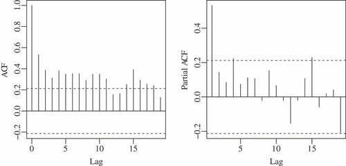
The mean of this series of flow data is 10 319.99 m³/s (standard deviation: 2522.07 m³/s). The sample autocorrelation function (ACF) (Fig. 7(a)) and the sample partial autocorrelation function (PACF) (Fig. 7(b)) indicate non-null autocorrelations in the time series. Nevertheless, the Pettitt test supposes independence of the dataset to its application. Therefore, we used a pre-whitening method, adapted from Serinaldi and Kilsby (2016), in the actual flow time series. This methodology consists of the following steps:

Figure 7. Observed (a) ACF and (b) PACF of the flow data.

Step1. The Pettitt test is applied to the original data. If there is no evidence to reject H₀, then there is “no change” and the analysis stopped.

Step2. If there is evidence to reject H₀, then the times series is split in two sub-series, $t=1,\dots ,\tau$ and $t=\tau +1,\dots ,T$. The difference of the means is computed by $\mathrm{\Delta }={\mu }_b-{\mu }_a$, and used to remove the step $x_t=y_t-\mathrm{\Delta }{.1}_{\{t>\tau \}}$.

Step3. The autocorrelation is removed by ${\epsilon }_t=x_t-{\hat{\rho }}^{\ast }{x}_{t-1}$, where

(9) ${\hat{\rho }}^{\ast }=\left(\hat{\rho }+\frac{1}{T}\right)\left(\frac{T}{T-3}\right)$(9)

with

(10) $\hat{\rho }=\frac{\frac{1}{\left(T-1\right)}{\sum }_{t=1}^{\left(T-1\right)}\left(X_t-\hat{\mu }\right)\left(X_{t+1}-\hat{\mu }\right)}{\frac{1}{T}{\sum }_{t=1}^T{\left(X_t-\hat{\mu }\right)}^2}$(10)

and

(11) $\hat{\mu }=\frac{1}{T}{\sum }_{t=1}^T{X}_t$(11)

Step4. Finally, the step change is combined with the uncorrelated series:

(12) $\hat{\mathrm{\Delta }}.1_{\{t>\tau \}}+\frac{{\epsilon }_t}{1-{\hat{\rho }}^{\ast }}$(12)

and the classical and proposed Pettitt tests are applied to this pre-whitened series.

By applying the Pettitt test and the proposed test in the complete series of flow data (T = 85), we obtained an identification of the change point for both tests, with p < 0.01. The change point was identified as being in 1971, as shown in Fig. 8. This result corroborates the results of the above-mentioned studies; the change in natural flow may have been caused by deforestation processes, the introduction of intensive agriculture, urban development (Tucci and Clarke 1998), or climate changes. As expected, we note a good performance of the classical Pettitt test in this application because (a) the sample size is large (T = 85), (b) the magnitude of the shift is big (S = 38.96%), and (c) the change point is almost in the midpoint of the series (τ = 48%).

Figure 8. Monthly average naturalized flow by year (solid line) and long-term average naturalized flow for the period before and after 1971 (dashed line).

However, a small data series is a reality in many monitoring stations, where the change point is not always located in the centre of the series. In order to mimic other real situations, we considered five different scenarios by making cuts in the original dataset. These scenarios are referred to as C1, C2, C3, C4 and C5, and their periods are described in Table 2. Scenario C1 is the only one that does not include the level change previously detected in the complete data. Scenario C2 presents the largest sample size among the five scenarios, while Scenario C5 has the smallest sample size (T = 32). Scenarios C4 and C5 are similar in relation to CV, τ and S, but have different sample sizes. The CV of the data in all scenarios ranges from 19.3 to 28.7%. The results of application of the tests for each scenario are also presented in Table 2. For both the classical Pettitt test and the proposed test, we considered significance levels equal to 5% (α = 0.05). If either the classical Pettitt test or the improved test did not reject the null hypothesis for C1 in Step 1 of the Serinaldi and Kilsby (2016) methodology, then the analysis was stopped.

Table 2. Application of the classical Pettitt test (P.T.) and the proposed test (P.T.*) to different samples from the Itaipu annual monthly flow data. T: sample size; CV: coefficient of variation of the sample; S: magnitude of the shift.

				P.T.		P.T.*		Change point (τ)
Scenario and period		T	CV (%)	p value	Detection	p value	Detection	(%)	Year	S (%)
C1	1931–1969	39	19.3	0.68831^a	NO	0.53247^a	NO	–	–	–
C2	1931–1990^b	60	27.1	0.00101	YES	0.00099	YES	68	1971	40.1
C3	1945–1986^b	42	28.7	0.07147	NO	0.04196	YES	64	1971	39.8
C4	1961–2015^b	55	20.5	0.01296	YES	0.00499	YES	30	1977	21.8
C5	1965–1996^b	32	23.5	0.09032	NO	0.04795	YES	39	1977	21.8

^ap value of P.T. and P.T.* to the original data.

^bwith change point detected in the complete data series.

The results presented in Table 2 show that the classical Pettitt test did not reject the null hypothesis for C3 (1945–1986) and C5 (1965–1968), i.e. it did not identify significant change in the mean of the series, unlike the test that uses the bootstrap method. For both scenarios, the time series includes the change point, the year 1971, at the extremity of the series. The proposed test was able to detect this change point, with p < 5%. These cases highlight that the detection performance of the proposed test is greater than that of the classical Pettitt test for short series, especially when the change point is far from the midpoint. Both tests rejected the null hypothesis for C2 and C4. These scenarios are related to large sample size, so it was expected that the classical Pettitt test would be able to identify the change. This result is in accordance with that previously obtained by Monte Carlo simulation.

It should be noted that in real data applications it is not always possible to choose the best range and sample size of the data. Then, if an inadequate test is applied, the results could lead to the wrong conclusions about the presence or absence of any change point(s).

6 Conclusions

In this study, we proposed an application of the Pettitt test via the bootstrap method. We examined the performance of both tests – the classical and proposed Pettitt tests – in identifying a change point in synthetic hydroclimatological data series using different scenarios through Monte Carlo simulation. We defined scenarios in order to incorporate a wide spectrum of possibilities, easily found in real data and with a view to contemplating short series, already identified as inadequate for the application of the classical Pettitt test.

The simulation results identified the size distortion of the Pettitt test, which was corrected or minimized through the bootstrap method application. By correcting the test size we obtained a more accurate and reliable detection, with Type I error probability closer to the significance level. Even with the correction of size distortions, the proposed test is also more powerful than the classical Pettitt test for detection of change points.

As a case study, we applied this to the flow data from the Itaipu Hydroelectric Plant. The results of this application corroborate the simulation results. The bootstrap Pettitt test can be useful in real situations because it is more reliable than the classical Pettitt test, particularly for small samples. When hydroclimatological data are important for society it is important to be able to quickly detect an abrupt change in order to support decision making for hydroclimatological resources management.

Disclosure statement

No potential conflict of interest was reported by the authors.

Additional information

Funding

We gratefully acknowledge partial financial support from Conselho Nacional de Desenvolvimento Cientıfico e Tecnológico (CNPq), Fundação de Amparo à Pesquisa do Estado do Rio Grande do Sul (FAPERGS) and Coordenação de Aperfeiçoamento de Pessoal de Nível Superior (CAPES), Brazil.

Appendix A

The probability distributions used in the simulation study described in Section 4 are described below.

A1 Gamma distribution

Let X be a random variable with a gamma distribution, the probability density function of X is given by (Montgomery and Runger 2006):

(A1) $f\left(x,\lambda ,\theta \right)=\frac{{\lambda }^{\theta }{x}^{\theta -1}{\mathrm{e}}^{-\lambda x}}{\mathrm{\Gamma }\left(\theta \right)},x>0$(A1)

where λ > 0 and θ > 0 are the parameters, $\mathrm{E}\left(X\right)=\frac{\theta }{\lambda }$ and $\mathrm{v}\mathrm{a}\mathrm{r}\left(X\right)=\frac{\theta }{{\lambda }^2}$.

A2 Gumbel distribution

The probability density function of the Gumbel distribution is given by (Chow 1964):

(A2) $f\left(x;\lambda ,\theta \right)=\frac{1}{\lambda }\mathrm{e}\mathrm{x}\mathrm{p}\left[-\frac{1}{\lambda }\left(x-\theta \right)-\mathrm{e}\mathrm{x}\mathrm{p}\left[-\frac{1}{\lambda }\left(x-\theta \right)\right]\right],-\mathrm{\infty }<x<\mathrm{\infty }$(A2)

where λ > 0 and $-\mathrm{\infty }<x<\mathrm{\infty }$ are the parameters, $\mathrm{E}\left(X\right)=\theta +\frac{\gamma }{\lambda }$ and $\mathrm{v}\mathrm{a}\mathrm{r}\left(X\right)=\frac{{\pi }^2}{6{\lambda }^2}$, where γ is the Euler constant (approx. 0.577).

A3 Normal distribution

The normal distribution is one of the most commonly used distributions in statistical modelling, assuming a symmetric bell shape (Walpole et al. 2006). It has as a characteristic data distribution with support from $-\mathrm{\infty }<x<\mathrm{\infty }$, which is what leads to the exclusion of several hydrological variables such as flow, precipitation and humidity, because there is no possibility of negative observations. The probability density function of this distribution is given by (Montgomery and Runger 2006):

(A3) $f\left(x;\mu ,{\sigma }^2\right)=\frac{1}{\sigma \sqrt{2\pi }}\mathrm{e}\mathrm{x}\mathrm{p}\left[\frac{-{\left(x-\mu \right)}^2}{2{\sigma }^2}\right],-\mathrm{\infty }<x<\mathrm{\infty }$(A3)

where $-\mathrm{\infty }<x<\mathrm{\infty }$ is the mean and ${\sigma }^2>0$ is the variance.

Appendix B

Tables B1 and B2 present the results obtained for Gumbel and normal distribution, respectively (cf. Table 1 for gamma distribution).

Table B1. Evaluation of the Pettitt test size (P.T.) and of the proposed test size (P.T.*) for Gumbel distribution. CV: coefficient of variation; α: significance level; and T: sample length.

	5%		10%		20%		30%
CV	P.T.	P.T.*	P.T.	P.T.*	P.T.	P.T.*	P.T.	P.T.*
α = 0.01
T = 10	0.0000	0.0080	0.0000	0.0076	0.0000	0.0090	0.0000	0.0084
T = 20	0.0015	0.0093	0.0017	0.0094	0.0011	0.0097	0.0018	0.0105
T = 30	0.0031	0.0112	0.0033	0.0100	0.0027	0.0095	0.0029	0.0090
T = 50	0.0035	0.0091	0.0048	0.0104	0.0046	0.0113	0.0044	0.0093
T = 100	0.0059	0.0099	0.0053	0.0101	0.0057	0.0098	0.0046	0.0080
α = 0.05
T = 10	0.0000	0.0441	0.0000	0.0417	0.0000	0.0436	0.0000	0.0412
T = 20	0.0168	0.0497	0.0180	0.0505	0.0186	0.0477	0.0202	0.0534
T = 30	0.0230	0.0489	0.0250	0.0506	0.0229	0.0483	0.0205	0.0470
T = 50	0.0290	0.0482	0.0316	0.0531	0.0295	0.0498	0.0290	0.0518
T = 100	0.0353	0.0486	0.0332	0.0485	0.0368	0.0519	0.0382	0.0527
α = 0.10
T = 10	0.0240	0.0937	0.0225	0.0933	0.0233	0.0959	0.0226	0.0895
T = 20	0.0463	0.1019	0.0471	0.0969	0.0439	0.1009	0.0492	0.1029
T = 30	0.0508	0.0962	0.0523	0.1021	0.0533	0.1006	0.0524	0.0981
T = 50	0.0578	0.0940	0.0683	0.1049	0.0647	0.1009	0.0647	0.1014
T = 100	0.0723	0.0994	0.0767	0.1038	0.0745	0.0994	0.0745	0.0988

Table B2. Evaluation of the Pettitt test size (P.T.) and the proposed test (P.T.*) for normal distribution. CV: coefficient of variation; α: significance level; and T: sample length.

	5%		10%		20%		30%
CV	P.T.	P.T.*	P.T.	P.T.*	P.T.	P.T.*	P.T.	P.T.*
α = 0.01
T = 10	0.0000	0.0100	0.0000	0.0075	0.0000	0.0080	0.0000	0.0078
T = 20	0.0010	0.0092	0.0015	0.0093	0.0015	0.0093	0.0012	0.0094
T = 30	0.0015	0.0077	0.0027	0.0092	0.0029	0.0105	0.0035	0.0102
T = 50	0.0040	0.0112	0.0044	0.0106	0.0037	0.0099	0.0051	0.0113
T = 100	0.0053	0.0096	0.0050	0.0073	0.0061	0.0098	0.0065	0.0113
α = 0.05
T = 10	0.0000	0.0434	0.0000	0.0445	0.0000	0.0447	0.0000	0.0473
T = 20	0.0168	0.0460	0.0176	0.0491	0.0193	0.0518	0.0167	0.0454
T = 30	0.0237	0.0499	0.0211	0.0455	0.0212	0.0470	0.0236	0.0513
T = 50	0.0299	0.0508	0.0321	0.0503	0.0283	0.0471	0.0290	0.0491
T = 100	0.0329	0.0466	0.0336	0.0496	0.0343	0.0471	0.0393	0.0521
α = 0.10
T = 10	0.0256	0.0990	0.0264	0.1016	0.0246	0.0974	0.0235	0.0933
T = 20	0.0464	0.0992	0.0438	0.0975	0.0453	0.1016	0.0469	0.1004
T = 30	0.0497	0.0949	0.0483	0.0952	0.0503	0.0918	0.0597	0.1037
T = 50	0.0630	0.1028	0.0634	0.0959	0.0572	0.0950	0.0638	0.0966
T = 100	0.0744	0.1008	0.0775	0.1021	0.0766	0.1027	0.0731	0.1003

Appendix C

The results of comparing the power of the tests to the different magnitudes of shift evaluated in this study are presented for: T = 10 (Fig. C1), T = 20 (Fig. C2), T = 30 (Fig. C3), T = 50 (Fig. C4) and T = 100 (Fig. C5). A significance level of α = 0.05 was established for all scenarios, with CV = 5% and gamma distribution.

Figure C2. Power of the tests for the different magnitudes of shift evaluated for T = 20: (a) change point in 10%; (b) change point in 50%; and (c) change point in 70%.

Figure C3. Power of the tests for the different magnitudes of shift evaluated for T = 30: (a) change point in 10%; (b) change point in 50%; and (c) change point in 70%.

Figure C4. Power of the tests for the different magnitudes of shift evaluated for T = 50: (a) change point in 10%; (b) change point in 50%; and (c) change point in 70%.

Figure C5. Power of the tests for the different magnitudes of shift evaluated for T = 100: (a) change point in 10%; (b) change point in 50%; and (c) change point in 70%.

References

- Aksoy, H., 2000. Use of gamma distribution in hydrological analysis. Turkish Journal of Engineering and Environmental Sciences, 24 (6), 419–428.
- Alley, R.B., et al., 2003. Abrupt climate change. Science, 299 (5615), 2005–2010. doi:10.1126/science.1081056
- Andreássian, V., 2004. Water and forests: from historical controversy to scientific debate. Journal of Hydrology, 291 (1–2), 1–27. doi:10.1016/j.jhydrol.2003.12.015
- Bayer, D.M. and Collischonn, W., 2013. Deforestation impacts on discharge of the Ji-Paraná River - Brazilian Amazon. In: E. Boegh, et al., eds. Climate and land surface changes in hydrology. 359th ed. Gothenburg: IAHS Publication, H01, 327–332.
- Beaulieu, C., Chen, J., and Sarmiento, J.L., 2012. Change-point analysis as a tool to detect abrupt climate variations. Philosophical Transactions of the Royal Society, 370, 1228–1249. doi:10.1098/rsta.2011.0383
- Bettolli, M.L. and Penalba, O.C., 2018. Statistical downscaling of daily precipitation and temperatures in southern La Plata Basin. International Journal of Climatology, 38 (9), 3705–3722. doi:10.1002/joc.2018.38.issue-9
- Bosch, J.M. and Hewlett, J.D., 1982. A review of catchment experiment to determine the effect of vegetation changes on water yield and evapotranspiration. Journal of Hydrology, 55 (1–4), 3–23. doi:10.1016/0022-1694(82)90117-2
- Boulanger, J.-P., et al., 2005. Observed precipitation in the Paraná - Plata hydrological basin: long-term trends, extreme conditions and ENSO teleconnections. Climate Dynamics, 24 (4), 393–413. doi:10.1007/s00382-004-0514-x
- Brannstrom, C., et al., 2008. Land change in the Brazilian Savanna (Cerrado), 1986–2002: comparative analysis and implications for land-use policy. Land Use Policy, 25 (4), 579–595. doi:10.1016/j.landusepol.2007.11.008
- Brown, A.E., et al., 2013. Impact of forest cover changes on annual streamflow and flow duration curve. Journal of Hydrology, 483, 39–50. doi:10.1016/j.jhydrol.2012.12.031
- Buishand, T.A., 1982. Some methods for testing the homogeneity of rainfall records. Journal of Hydrology, 58 (1–2), 11–27. doi:10.1016/0022-1694(82)90066-X
- Busuioc, A. and von Storch, H., 1996. Changes in the winter precipitation in Romania and its relation to the large-scale circulation. Tellus, 48 (4), 538–552. doi:10.1034/j.1600-0870.1996.t01-3-00004.x
- Cavalcanti, I.F.A., et al., 2015. Precipitation extremes over La Plata Basin – review and new results from observations and climate simulations. Journal of Hydrology, 523, 211–230. doi:10.1016/j.jhydrol.2015.01.028
- Chandler, R.E. and Scott, M., 2011. Statistical methods for trend detection and analysis in the environmental sciences. Chichester, UK: John Wiley & Sons Ltd.
- Chow, V.T., 1964. Handbook of applied hydrology. Vol. 1, New York: McGraw-Hill.
- Dailidiené, I., et al., 2011. Long term water level and surface temperature changes in the lagoons of the southern and eastern Baltic. Oceanologia, 53 (1), 293–308. doi:10.5697/oc.53-1-TI.293
- Davison, A.C. and Hinkley, D.V., 1997. Bootstrap methods and their application. Cambridge Series in Statistical and Probabilistic Mathematics. Cambridge, UK: Cambridge University Press.
- Doyle, M.E. and Barros, V.R., 2011. Attribution of the river flow growth in the Plata Basin. International Journal of Climatology, 31 (15), 2234–2248. doi:10.1002/joc.v31.15
- Efron, B. and Tibshirani, R.J., 1994. An introduction to the bootstrap. Chapman & Hall/CRC Monographs on Statistics & Applied Probability. New York, NY: Taylor & Francis.
- Fu, G., et al., 2004. Hydro-climatic trends of the Yellow river basin for the last 50 years. Climatic Change, 65 (1), 149–178. doi:10.1023/B:CLIM.0000037491.95395.bb
- Gao, P., et al., 2015. Streamflow regimes of the yanhe river under climate and land use change, Loess Plateau, China. Hydrological Processes, 29 (10), 2402–2413. doi:10.1002/hyp.10309
- Garcı́a, N.O. and Vargas, W.M., 1998. The temporal climatic variability in the “Rı́o de La Plata” basin displayed by the river discharges. Climatic Change, 38 (3), 359–379. doi:10.1023/A:1005386530866
- Garcı́a, N.O., Vargas, W.M., and Del Valle Venencio, M., 2002. About of the 1970/71 climatic jump on the “Rı́o de La Plata” basin. In: Land atmosphere interactions, 16th Conference on Hydrology and 13th Symposium on Global Change and Climate Variations. No. JP1.11, Orlando, 1 p.
- INMET (Instituto Nacional de Meteorologia), 1992. Normais climatologicas do Brasil 1961–1990 [online]. http://www.inmet.gov.br/portal/index.php?r=clima/normaisclimatologicas [Accessed June 2017].
- IPCC (Intergovernmental Panel on Climate Change), 1992. Climate Change: The 1990 and 1992 IPCC assessments. First assessment report overview and policy-maker summaries and 1992 IPPC supplement. Technical report. Geneva, Switzerland: UNEP and WMO.
- IPCC, 1995. IPCC second assessment climate change 1995. A report of the Intergovernmental Panel on Climate Change. Technical report. Geneva, Switzerland: UNEP and WMO.
- IPCC, 2001. Climate change 2001: the scientific basis. Contribution of Working Group I to the Third Assessment Report of the Intergovernmental Panel on Climate Change. UNEP and WMO. Cambridge, UK and New York, NY: Cambridge University Press.
- IPCC, 2007. Climate change 2007: synthesis report. Contribution of working groups I, II and III to the Fourth Assessment Report of the Intergovernmental Panel on Climate Change. Technical report. Geneva, Switzerland: UNEP and WMO.
- IPCC, 2014. Climate change 2014: synthesis report. Contribution of working groups I, II and III to the Fifth Assessment Report of the Intergovernmental Panel on Climate Change. Technical report. Geneva, Switzerland: WMO and UNEP.
- IPCC, 2018. Summary for policymakers. In: Global warming of 1.5ºC. An IPCC Special Report on the impacts of global warming of 1.5ºC above pre-industrial levels and related global greenhouse gas emission pathways, in the context of strengthening the global response to the threat of climate change, sustainable development, and efforts to eradicate poverty (V. Masson-Delmotte et al., Eds.). Geneva, Switzerland: World Meteorological Organization.
- ITAIPU, 2019. Itaipu binacional [online]. https://www.itaipu.gov.br/ [Accessed January 2019].
- Jiang, S., et al., 2011. Quantifying the effects of climate variability and human activities on runoff from the Laohahe basin in northern China using three different methods. Hydrological Processes, 25 (16), 2492–2505. doi:10.1002/hyp.v25.16
- Karabörk, M., Kahya, E., and Kömüşçü, A.U., 2007. Analysis of Turkish precipitation data: homogeneity and the Southern Oscillation forcings on frequency distributions. Hydrological Processes, 21 (23), 3203–3210. doi:10.1002/hyp.6524
- Kruskal, W.H. and Wallis, A.W., 1952. Use of ranks in one-criterion variance analysis. Journal of the American Statistical Association, 47 (260), 583–621. doi:10.1080/01621459.1952.10483441
- Kundzewicz, Z.W. and Robson, A., 2000. Detecting trend and other changes in hydrological data. Technical report. Geneva, Switzerland: World Climate Programme-Water.
- Kundzewicz, Z.W. and Robson, A., 2004. Change detection in hydrological records - a review of the methodology. Hydrological Sciences Journal, 49 (1), 7–19. doi:10.1623/hysj.49.1.7.53993
- Leese, M.N., 1973. Use of censored data in the estimation of Gumbel distribution parameters for annual maximum flood series. Water Resources Research, 9 (6), 1534–1542. doi:10.1029/WR009i006p01534
- Liu, D., et al., 2010. Impacts of climate change and human activities on surface runoff in the Dongjiang River basin of China. Hydrological Processes, 24 (11), 1487–1495. doi:10.1002/hyp.v24:11
- Liu, L., Xu, Z.-X., and Huang, J.-X., 2012. Spatio-temporal variation and abrupt changes for major climate variables in the Taihu basin, China. Stochastic Environmental Research and Risk Assessment, 26 (6), 777–791. doi:10.1007/s00477-011-0547-8
- Loucks, D.P. and van Beek, E. with contributions from Jery R Stedinger, E., Dijkman, J. P. M., Villars, M. T., 2005. Water resources systems planning and management. Paris, France: United Nations Educational, Scientific and Cultural Organization – UNESCO.
- Mallakpour, I. and Villarini, G., 2016. A simulation study to examine the sensitivity of the Pettitt test to detect abrupt changes in mean. Hydrological Sciences Journal, 61 (2), 245–254. doi:10.1080/02626667.2015.1008482
- Mann, H.B. and Whitney, D.R., 1947. On a test of whether one of two random variables is stochastically larger than the other. The Annals of Mathematical Statistics, 18 (1), 50–60. doi:10.1214/aoms/1177730491
- Montgomery, D.C. and Runger, G.C., 2006. Applied statistics and probability for engineers. 4th ed. Wiley. National Academies of Sciences, E., Medicine, 2016. Attribution of Extreme Weather Events in the Context of Climate Change. Washington, DC: The National Academies Press.
- Montroull, N.B., Saurral, R.I., and Camilloni, I.A., 2018. Hydrological impacts in La Plata basin under 1.5, 2 and 3 ºC global warming above the pre-industrial level. International Journal of Climatology, 38 (8), 3355–3368. doi:10.1002/joc.5505
- National Academy of Sciences, 2002. Abrupt climate change: inevitable surprises. Washington, DC: Committee on Abrupt Climate Change, Ocean Studies Board, Polar Research Board, Board on Atmospheric Sciences and Climate, Division on Earth and Life Studies, National Research Council.
- National Research Council, 2010. Assessment of intraseasonal to interannual climate prediction and predictability. Washington, DC: The National Academies Press.
- Nóbrega, R.L.B., et al., 2018. Impacts of land-use and land-cover change on stream hydrochemistry in the Cerrado and Amazon biomes. Science of the Total Environment, 635, 259–274. doi:10.1016/j.scitotenv.2018.03.356
- ONS, 2017. Séries históricas de vazões [online]. http://ons.org.br/Paginas/resultados-da-operacao/historico-da-operacao/dados_hidrologicos_vazoes.aspx [Accessed June 2017].
- ONS, 2019. Glossário [online]. http://ons.org.br/paginas/conhecimento/glossario [Accessed January 2019].
- Pettitt, A.N., 1979. A non-parametric approach to the change-point problem. Journal of the Royal Statistical Society: Series C (Applied Statistics), 28 (2), 126–135.
- Puig, A., Salinas, H.F.O., and Borús, J.A., 2016. Recent changes (1973–2014 versus 1903–1972) in the flow regime of the lower Paraná river and current fluvial pollution warnings in its Delta biosphere reserve. Environmental Science and Pollution Research, 23 (12), 11471–11492. doi:10.1007/s11356-016-6501-z
- R Core Team, 2017. R: a language and environment for statistical computing. Vienna, Austria: R Foundation for Statistical Computing. https://www.R-project.org/
- Reis, S. and Yilmaz, H.M., 2008. Temporal monitoring of water level changes in Seyfe Lake using remote sensing. Hydrological Processes, 22 (22), 4448–4454. doi:10.1002/hyp.v22:22
- Rizzo, M.L., 2007. Statistical computing with R. New York, NY: Chapman & Hall/CRC.
- Rosenzweig, C., et al., 2008. Attributing physical and biological impacts to anthropogenic climate change. Nature Publishing Group, 453, 353–358.
- Rougé, C., Ge, Y., and Cai, X., 2013. Detecting gradual and abrupt changes in hydrological records. Advances in Water Resources, 53, 33–44. doi:10.1016/j.advwatres.2012.09.008
- Serinaldi, F. and Kilsby, C.G., 2016. The importance of prewhitening in change point analysis under persistence. Stochastic Environmental Research and Risk Assessment, 30 (2), 763–777. doi:10.1007/s00477-015-1041-5
- Suhaila, J. and Yusop, Z., 2017. Trend analysis and change point detection of annual and seasonal temperature series in Peninsular Malaysia. Meteorology and Atmospheric Physics, 130 (5), 565–581. doi:10.1007/s00703-017-0537-6
- Tarhule, A. and Woo, M.-K., 1998. Changes in rainfall characteristics in northern Nigeria. International Journal of Climatology, 18 (11), 1261–1271. doi:10.1002/(ISSN)1097-0088
- Tucci, C.E.M. and Clarke, R.T., 1998. Environmental issues in the La Plata basin. International Journal of Water Resources Development, 14 (2), 157–173. doi:10.1080/07900629849376
- UNDP, 2007. Human development report 2007/2008: fighting climate change: human solidarity in a divided world. London: Palgrave Macmillan.
- Villarini, G., et al., 2009. On the stationarity of annual flood peaks in the continental United States during the 20th century. Water Resources Research, 45 (8), 1–17. doi:10.1029/2008WR007645
- Villarini, G. and Smith, J.A., 2010. Flood peak distributions for the eastern United States. Water Resources Research, 46 (6), 1–17. doi:10.1029/2009WR008395
- Walpole, R.E., et al., 2006. Probability & statistics for engineers & scientists. 8th ed. London, UK: Prentice Hall.
- Wang, W., et al., 2013. Quantitative assessment of the impact of climate variability and human activities on runoff changes: a case study in four catchments of the Haihe River basin, China. Hydrological Processes, 27 (8), 1158–1174. doi:10.1002/hyp.9299
- Wang, Y.-J. and Qin, D.-H., 2017. Influence of climate change and human activity on water resources in arid region of northwest china: an overview. Advances in Climate Change Research, 8 (4), 268–278. doi:10.1016/j.accre.2017.08.004
- Wijngaard, J.B., Tank, A.M.G.K., and Konnen, G.P., 2003. Homogeneity of 20th century European daily temperature and precipitation series. International Journal of Climatology, 23 (6), 679–692. doi:10.1002/joc.906
- WMO (World Meteorological Organization), 1988. Analysing long time series of hydrological data with respect to climate variability. Technical report 224. WMO.
- WMO, 2016. WMO statement on the state of the global climate in 2016. Technical report 1189. WMO.
- Worsley, K.J., 1979. On the likelihood ratio test for a shift in location of normal populations. Journal of the American Statistical Association, 74 (366a), 365–367.
- Xie, H., Li, D., and Xiong, L., 2014. Exploring the ability of the Pettitt method for detecting change point by Monte Carlo simulation. Stochastic Environmental Research and Risk Assessment, 28 (7), 1643–1655. doi:10.1007/s00477-013-0814-y
- Yoo, C., Jung, K.-S., and Kim, T.-W., 2005. Rainfall frequency analysis using a mixed gamma distribution: evaluation of the global warming effect on daily rainfall. Hydrological Processes, 19 (19), 3851–3861. doi:10.1002/(ISSN)1099-1085
- Yue, S., et al., 1999. The Gumbel mixed model for flood frequency analysis. Journal of Hydrology, 226 (1–2), 88–100. doi:10.1016/S0022-1694(99)00168-7
- Yue, S., Ouarda, T.B.M.J., and Bobée, B., 2001. A review of bivariate gamma distribution for hydrological application. Journal of Hydrology, 246 (1), 1–18. doi:10.1016/S0022-1694(01)00374-2
- Zhang, M., et al., 2017. A global review on hydrological responses to forest change across multiple spatial scales: importance of scale, climate, forest type and hydrological regime. Journal of Hydrology, 546, 44–59. doi:10.1016/j.jhydrol.2016.12.040
- Zhang, X., et al., 2007. Detection of human influence on twentieth-century precipitation trends. Nature Publishing Group, 448, 461–466.
- Zuo, D., et al., 2012. Spatiotemporal variations and abrupt changes of potential evapotranspiration and its sensitivity to key meteorological variables in the Wei River basin, China. Hydrological Processes, 26 (8), 1149–1160. doi:10.1002/hyp.8206