Climatic effects on ice phenology and ice-jam flooding of the Athabasca River in western Canada

ABSTRACT

In cold region environments, any alteration in the hydro-climatic regime can have profound impacts on river ice processes. This paper studies the implications of hydro-climatic trends on river ice processes, particularly on the freeze-up and ice-cover breakup along the Athabasca River in Fort McMurray in western Canada, which is an area very prone to ice-jam flooding. Using a stochastic approach in a one-dimensional hydrodynamic river ice model, a relationship between overbank flow and breakup discharge is established. Furthermore, the likelihood of ice-jam flooding in the future (2041–2070 period) is assessed by forcing a hydrological model with meteorological inputs from the Canadian regional climate model driven by two atmospheric–ocean general circulation climate models. Our results show that the probability of ice-jam flooding for the town of Fort McMurray in the future will be lower, but extreme ice-jam flood events are still probable.

KEYWORDS:

• ice-jam floods
• hydro-climatic trends
• ice phenology
• flood risk
• Athabasca River
• Canada

Editor R. Woods; Associate editor S. Vorogushyn

1 Introduction

In cold region hydrology, river ice plays a major role in the hydrological regime, which in turn influences physical, chemical and biological processes. For instance, a stable ice cover can cause additional resistance and reduce flow velocities, whereas in some shallow channel systems, groundwater flows can be blocked if ice freezes to the bed (Beltaos and Burrell 2003). Thus, ice cover formation and breakups are important cold region processes in northern rivers. However, ice-jamming and subsequent breakup events (depending upon hydro-meteorological conditions and river ice properties) can also be disastrous to riverine communities. Ice-jam floods (IJFs) can be particularly dangerous since they can occur very rapidly, and are often associated with water levels higher than those attained during open-water flooding conditions. The water depths have been reported to be as high as 2.5–3 times the regular open-water level at the same discharge during such ice-jamming conditions (Beltaos and Prowse 2001).

However, as in other cold regions across the globe, the interior of western Canada is observing rapid warming, which has significant impacts in terms of hydrological and landscape change. Though major river systems, such as the Mackenzie and Nelson rivers, have shown no noticeable long-term trends at their mouths (Déry et al. 2011), some smaller systems nested within these, such as the Athabasca River and other rivers draining from the Rocky Mountains to the south, have shown statistically significant declines in annual flow since the late 1950s (DeBeer et al. 2016). Peters et al. (2013) performed a multi-scale hydro-climatic analysis of runoff in the Athabasca River basin (ARB) and found a decreasing streamflow pattern since 1958 in the lower reaches. Similar results were reported by Bawden et al. (2014), who showed declining trends in different hydrological variables. Monk et al. (2012) also reported decreasing trends in ecologically relevant hydrological variables, such as short‐term and long‐term maximum and minimum runoff, since 1958. But the findings of a century-long record from Rood et al. (2015) showed statistically significant decreasing trends only in headwaters. Though they did not find statistically significant trends in the lower basin, they also acknowledged significant declines in flows since 1970. Since any alteration in hydrological regime can have profound impacts on the composition, thickness, severity and timing of river ice processes, it is imperative to understand and assess the implications of current and future hydro-climatic trends on river ice processes in the ARB and particularly for the ice-jam flood prone location, the town of Fort McMurray (TFM) which is a key motivation for this research and has been missing in above mentioned hydro-climatic studies.

Frequent and severe ice jams during the breakup period have been observed in the past along different reaches of the Athabasca River. Historical records show that there has been about one IJF every five years over the period 1875–2012 along the Athabasca River (Rokaya 2018). Although IJFs have occurred along different reaches of the Athabasca River, IJF events are more prominent near the TFM due to the river reach’s gentle riverbed slope and the presence of numerous islands and bars. Since the gauging station was installed at the TFM in late 1957, 15 ice-jam floods have been recorded along the Athabasca River, the majority (60%) of which occurred at the TFM resulting in loss of millions of dollars in direct and indirect damages. The 1977 ice-jam flooding of the TFM caused Can$2.6 million of damage claims, whereas the 1997 event is estimated to have resulted in several millions dollars of damage (Mahabir et al. 2006).

Some ice-jam breakup events in the ARB have been studied in recent years, especially those occurring at the TFM. These include events in 1977–1979 (Andres and Doyle 1984), 2001–2003 (Hutchison and Hicks 2007) and 2006–2007 (She et al. 2009). However, the potential impacts of reduced streamflows and other hydro-climatic variability in recent decades on river ice processes (such as ice formation, breakup and jamming) have not been fully investigated. Future climate change impacts on hydrology (Kerkhoven and Gan 2011), snow water equivalent (Dibike et al. 2018a), hydrological indicators (Eum et al. 2017) and water availability (Leong and Donner 2015) have also been assessed, but potential implications on river ice processes, especially on ice-jam floods, have not been examined. Thus, the specific objectives of this research are to: (a) assess the impacts of historical hydro-climatic trends on river ice processes; (b) approximate a flow threshold required for IJF; and (c) estimate the probabilities of ice-jam flooding of the TFM in the future.

First, a non-parametric Mann-Kendall trend test (Mann 1945) was used to analyse the trends in river ice cover formation and breakup after removing first order autocorrelation. The one-dimensional hydrodynamic model RIVICE (ECCC 2013) was then applied to assess probabilities of overbank flow based on breakup discharge under ice-jam conditions using a stochastic method. And finally, MESH, a land-surface and hydrology modelling system (Pietroniro et al. 2007) was implemented to examine the potential future discharges at freeze-up and breakup periods, as well as to assess the likelihood of IJFs in the future (2041–2070 period). The results show that the probability of IJFs along the Athabasca River at the TFM in the future will be lower, but extreme IJF events are still probable.

2 Data and methods

2.1 Study area

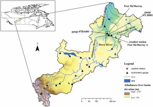
The Athabasca River originates in the Rocky Mountains of central Alberta (see Fig. 1) and spans the provinces of Alberta and Saskatchewan to drain over 150 000 km² of land area. The river initially flows through the mountainous and forested landscape of Jasper National Park and onwards through Brule Lake and Jasper Lake, into rolling foothills and continuing to Lake Athabasca (Peters et al. 2013). From Lake Athabasca, water flows northward via the Slave River to Great Slave Lake, the Mackenzie River, and the Arctic Ocean. The river is 1538 km long and the elevation ranges from 3747 m a.s.l. at its origin at Mount Columbia to 187 m a.s.l. at its terminal point at Lake Athabasca (Peters and Prowse 2006). The ARB has a continental climate with significant seasonal variations. The record from the period 1981–2010 for meteorological station “Fort McMurray A” shows that, on average, the daily mean temperature drops below freezing from the middle of October to early April, with an average January temperature of −17.4°C. The average temperature in July is 17.1°C. The annual precipitation for the same period averages around 400 mm, of which roughly 75% occurs as rain. The hydrological regime of the ARB is characterized by low flows in the winter months and a rising hydrograph starting in late April and May and peaking, generally, in June (Burn et al. 2004).

Figure 1. The location map of the study basin.

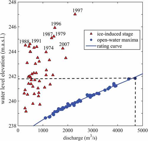
The TFM lies at the confluence of the Athabasca and Clearwater rivers. As the Athabasca River flows north past the town, changes in river morphology at the TFM make the river more conducive to ice jam flooding. The presence of several tributaries, including the Clearwater and Horse rivers, in this reach provide additional sources of water and ice which can exacerbate an already hazardous ice flood situation along the Athabasca River. Historical records show that the majority of IJFs in the ARB have occurred at the TFM. Figure 2 shows that ice-jam conditions can lead to significantly higher water levels at the TFM compared to the open-water period, despite having comparatively smaller river discharges. For instance, the largest open-water flood with a discharge above 4500 m³/s resulted in staging of less than 242 m a.s.l., whereas much higher staging were observed during ice-jam conditions when discharges were merely one-fifth of that.

Figure 2. Open-water rating curve for 1961–2012 period at the TFM (07DA001). The red triangles denote ice-induced instantaneous maximum water level whereas blue circle represent annual open-water maxima.

2.2 Flow and water level data

Daily discharge data were retrieved from the Water Survey of Canada (WSC) through the HYDAT database of Environment and Climate Change Canada (ECCC)¹ for several stations across the basins (see Fig. 1 and Table 1 for location and details of the gauges in the basin). The water level data were available from the WSC regional office in Alberta for the period 1958–2012. Some breakup water levels for the TFM were obtained from Sun and Trevor (2018). Meteorological data including air temperature are available from ECCC² and were extracted for the 1958–2012 period.

Table 1. Hydrometric stations in the ARB.

SN	Station ID	Station name	Latitude	Longitude	Ice-on data	Ice-off data
1	07AA001	Miette River near Jasper	52.8641	–118.107	1975–2012	1974–2012
2	07AA002	Athabasca River near Jasper	52.9101	–118.059	1970–2014	1971–2014
3	07AD002	Athabasca River at Hilton	53.4242	–117.569	1961–2014	1962–2014
4	07AF002	Mcleod River above Embarras River	53.4701	–116.632	1954–2013	1955–2013
5	07AG003	Wolf Creek at highway no. 16a	53.5983	–116.272	1954–2014	1955–2014
6	07BB002	Pembina River near Entwistle	53.6041	–115.005	1954–2012	1955–2012
7	07BC002	Pembina River at Jarvie	54.4502	–113.993	1957–2013	1958–2013
8	07BE001	Athabasca River at Athabasca	54.7220	–113.288	1951–2013	1952–2013
9	07BF002	West Prairie River near High Prairie	55.4482	–116.493	1969–2012	1959–2012
10	07BJ001	Swan River near Kinuso	55.3155	–115.417	1969–2012	1962–2012
11	07BK007	Driftwood River near the mouth	55.2554	–114.231	1970–2013	1968–2013
12	07CD001	Clearwater River at Draper	56.6852	–111.255	1957–2014	1958–2014
13	07CD005	Clearwater River above Christina river	56.6636	–110.929	1966–2014	1975–2014
14	07CE002	Christina River near Chard	55.8371	–110.869	1982–2014	1983–2014
15	07DA001	Athabasca River below Fort McMurray	56.7803	–111.402	1957–2014	1958–2014
16	07DB001	Mackay River near Fort Mackay	57.2103	–111.695	1972–2014	1973–2014
17	07DC001	Firebag River near the mouth	56.7803	–111.402	1971–2014	1972–2014

2.3 Ice-on and ice-off data, and freeze-up and breakup dates

Freeze-up is conceptually defined as “the time at which a continuous and immobile ice cover forms” (IPCC 2007). Breakups occur in spring when increasing temperature disintegrates the ice cover or increased flow dislodges it (Beltaos 1997). The WSC provides a “B” flag, along with the hydrometric data, to indicate “backwater” effects due to the presence of ice at or immediately downstream of the gauge in the river. Thus, the discharge with the first B flag indicates the beginning of the freeze-up of the river (ice-on) whereas the last B flag is indicative of the end of the ice cover season (ice-off). In our study, the freeze-up date is considered as the day with the highest water level within +3 days of the first B flag, and the breakup was assumed to be the date of the greatest water depth within −3 days of the last B flag (Rokaya et al. 2018a).

2.4 Trend analysis

A non-parametric Mann-Kendall (MK) trend test (Mann 1945) was used to detect trends in historical records of discharge, precipitation, air temperature, ice-on and ice-off dates, and freeze-up and breakup dates at multiple stations. The MK test is a widely-used methodology that can be more robust than other methods for skewed environmental data. However, autocorrelations of time series can inflate the statistical significance (i.e. the p value) of the MK test and its parametric counterparts. Serial autocorrelations were thus removed from the time series prior to the trend analysis using a method suggested by Zhang et al. (2000). Usually, the first-order autocorrelation is removed from the time series (Yue et al. 2002). In this analysis, the null hypothesis (H₀) was assumed as no trend (p > 0.05), which is tested against the alternative hypothesis H₁ of increasing or decreasing trends.

2.5 River ice modelling

2.5.1 RIVICE

RIVICE is a one-dimensional hydrodynamic model (ECCC 2013), which uses an implicit finite-difference numerical method to simulate river ice processes and phenomena, such as ice generation, ice transport, ice cover formation, hanging dam development and ice jam progression along the river. It simulates ice jams by coupling ice dynamics with river hydraulics as outputs from meteorological and river bathymetrical input parameters. The fundamental premise of the model structure is the loose coupling between the hydraulic and river ice computations, in which data are exchanged frequently, after every time step, to retain model accuracy without increasing the computational burden. Under conditions of very rapid ice cover formation, the time step varies from a few minutes to seconds to best capture these rapidly changing events. Further details on model structure, set-up and calibration can be found in the literature (Lindenschmidt et al. 2016, Sheikholeslami et al. 2017, Rokaya et al. 2018b).

2.5.2 Model set-up

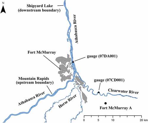
The RIVICE modelling domain extends 40 km along the Athabasca River from Mountain Rapids to near Shipyard Lake (see Fig. 3). This part of the river is characterized by rapids, as well as numerous sand bars and islands. The width of the river varies between 300 and 700 m, with slopes of approximately 0.0010 and 0.0003 in the upper and lower reaches, respectively. The TFM lies at the confluence of the Athabasca and Clearwater rivers. As the upper portion of the model domain is embedded within a very steep section with many rapids, a large supply of ice is generated and is available for ice-jam formation and breakup. The presence of several tributaries in this reach also provides additional sources of water and ice, which can exacerbate an already hazardous ice flood situation along the Athabasca River. The bathymetry data for this study were surveyed at different times in the period 1973–2002 to progressively fill in gaps and reduce the distance between cross-sections.

Figure 3. RIVICE modelling domain.

2.5.3 RIVICE calibration

Fort McMurray sustained extreme ice-jam flooding in the late 1970s with consecutive flooding in 1977, 1978 and 1979. These three events have been well documented and reported (see Doyle (1977); Andres and Doyle (1984)). First, the model was calibrated for an ice-jam flood event that occurred on 30 April 1979. It was then validated against an ice-jam flood event that took place on 16 April 1977. The ice-jam events were chosen based on the availability of water level and other hydrometric data and thus were used for model calibration and validation.

For calibration, the flow and water level boundary conditions were derived from the gauge data from the Athabasca (07DA001) and Clearwater (07CD001) rivers. Although gauge readings at the TFM showed a mean daily flow of 1480 m³/s, Andres and Doyle (1984) estimated the instantaneous flow to range between 1300 and 1850 m³/s. Lindenschmidt (2017) further revealed that the upstream discharge and the downstream water level were probably around 1366 m³/s and 235.5 m a.s.l, respectively, and these values were used in this study since Lindenschmidt (2017) was able to simulate the 1979 flood adequately with the above-mentioned upstream flow and downstream water level values. Eight parameters, the porosity of slush, thickness of slush pans, porosity of ice cover, thickness of ice cover front, ice roughness, river bed roughness, and lateral and longitudinal stresses, were calibrated based on previous RIVICE modelling of the Athabasca River (e.g. Lindenschmidt 2017) and sensitivity analyses of RIVICE parameters (e.g. Lindenschmidt and Chun 2013, Sheikholeslami et al. 2017). The bed and ice roughness parameters were calibrated separately. First, the bed roughness parameter was calibrated for the open-water simulation and then ice roughness calibrated for the ice-jam event. Data for boundary conditions include upstream discharge, downstream water level, incoming ice volume and the location of the toe of the ice-jam, which were obtained from gauge readings or previous publications (e.g. Doyle 1977, Andres and Doyle 1984). The model was run at a 30-s time step for numerical stability. Calibration was performed against recorded high-water marks of the flood event. The model performance was evaluated through visual inspection and comparing the Nash-Sutcliffe (NS) efficiency, mean absolute error (MAE), root mean square error (RMSE) and coefficient of determination (R²) between simulated and observed water levels.

The model was then validated using data from the 1977 ice-jam flood event. A daily flow of 934 m³/s was recorded at the TFM gauge. Lindenschmidt (2017) used an upstream discharge of 1000 m³/s, the downstream water level of 235 m a.s.l. and an incoming ice volume of 2000 m³/∆t, allowing successfully simulation of the 1977 ice-jam flood event. While the 1977 jam had occurred in the downstream reach, the 1979 jam occurred in the steep section of the upstream reach. The location of the toe of the jam was at 4 km upstream of the MacEwan Bridge (Andres and Doyle 1984) which is about 5 km upstream of the Clearwater River confluence. Initial values for rubble ice and ice cover properties, ice-jam characteristics and hydraulic roughness were obtained from the literature (e.g. Andres and Doyle 1984, Lindenschmidt 2017).

2.5.4 Monte Carlo simulations

After calibrating and validating the RIVICE model for the Athabasca River, 1000 ensembles of water level profiles were simulated within a Monte Carlo (MOCA) framework embedded in Model-Independent Parameter Estimation (PEST), an industry standard software package for parameter estimation and uncertainty analysis of complex environmental and other computer models (Doherty 1994). There are four major boundary conditions and eight model parameters whose distributions are essential to run RIVICE in a MOCA framework (see Fig. 4 for schematic view of calibration framework and Table 2 for a full list of parameters and their ranges). The boundary conditions included upstream discharge for the Athabasca and Clearwater rivers, the downstream water level in the Athabasca River, incoming ice volume and the location of the toe of the ice jam, whereas model parameters represent ice roughness, river bed roughness, porosity of slush, thickness of slush pans, porosity of ice cover, thickness of ice cover front and longitudinal and vertical stresses (Table 2).

Table 2. Ranges of parameter and boundary conditions used in RIVICE calibration and validation, as well as for MOCA simulations.

Parametersand boundary conditions	Description	Units	Lower bound	Upper bound
Parameters
PS	Porosity of slush	-	0.3	0.7
ST	Thickness of slush pans	m	0.1	0.3
PC	Porosity of ice cover	-	0.4	0.7
FT	Thickness of ice cover front	m	0.15	0.3
nice	Ice roughness	s/m^1/3	0.025	0.035
nbed	River bed roughness	s/m^1/3	0.020	0.030
K1TAN	Lateral: longitudinal stresses	-	0.11	0.22
K2	Longitudinal: vertical stresses	-	7	10
Boundary conditions
Qa	Upstream discharge of Athabasca River	m^3/s	806.7^a	508.5^b
Qc	Discharge from Clearwater River	m^3/s	252.8^a	125.7^b
Wds	Downstream water level	m a.s.l.	233	236
X	Location of the toe of the ice jam	chainage (m)	15000	30000
Vice	Incoming ice volume	m^3/Δt	2050^a	417^b

^a Location for Gumbel pdf.

^b Scale for Gumbel pdf.

Figure 4. The Monte Carlo simulation framework.

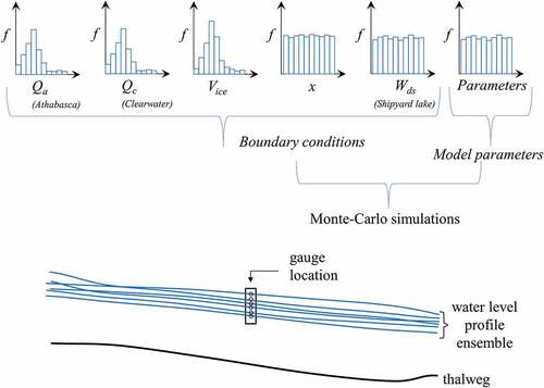
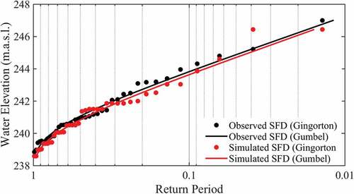
For both boundary conditions and model parameters the values were randomly extracted from the probability density functions (pdf) within certain ranges (uniform pdf) or range of location and scale factors (Gumbel pdf). When data were available to construct their pdfs (such as discharge and stages), the Gumbel function (Thompson 1999) was used but when a priori knowledge on pdf shape was not available (e.g. the toe of the ice jam location or model parameters), a uniform pdf was used. This method is discussed in detail by Rokaya et al. (2019). In this study, Gumbel distributions were used to generate random values for the upstream discharges for both the Athabasca and Clearwater rivers and downstream water level, whereas uniform distributions were considered for the location of the toe of the ice jam and model parameters as a priori knowledge on the pdf shape was not available. The lower and upper bounds for the model parameters were selected from the literature (e.g. Lindenschmidt 2017, Beltaos 2018) and through the calibration and validation process of the RIVICE model. The incoming ice volume was calibrated against the maximum instantaneous ice jam stage frequency curve within the framework of a MOCA analysis. Using mean and standard deviation to derive location and scale parameters, a Gumbel distribution of ice volume was generated until the resulting simulated ice-jam stage frequency matched the stage frequency curve of the recorded water levels at the gauging station (see Fig. 5).

Figure 5. Simulated and observed ice-jam stage frequency distributions (Gumbel) with plotting positions (Gringorton) for the gauge at Fort McMurray (07DA001).

2.6 Hydrological modelling

2.6.1 MESH

MESH (Modélisation Environmentale–Surface et Hydrologie) is a semi-distributed physically-based land surface–hydrological modelling system developed by ECCC for hydrological applications (Pietroniro et al. 2007). It uses the Canadian Land Surface Scheme (CLASS) for vertical exchanges and generation of lateral fluxes of energy and water balance for vegetation, soil and snow; the WATROUTE or PDMROF module to simulate lateral flows; and the WATFLOOD module for flow routing. It also uses the Group Response Unit (GRU) approach, i.e. combining areas of similar hydrological behaviour, to address the complexity and heterogeneity in the drainage basin for computational efficiency (Kouwen et al. 1993). This has been found to be a more suitable approach for large-scale drainage basins due to its operational simplicity, while retaining the basic physics and behaviour of a distributed model (Pietroniro and Soulis 2003).

2.6.2 MESH set-up

A hydrological model using MESH was set up for the ARB with a spatial resolution of 0.125°, resulting in 1326 grids, with the outlet of the basin delineated at the gauge Athabasca River below Fort McMurray (07DA001, see Fig. 1). The drainage database was prepared using GreenKenue (Canadian Hydraulics Centre 2010), an advanced data preparation, analysis, and visualization tool. The topographic data were obtained from the Canadian Digital Elevation Data. The land-use data were retrieved from Natural Resource Canada and soil data from Soil Landscapes of Canada. Further details on the model set-up are given in Morales-Marín et al. (2019).

2.6.3 Meteorological forcing data

The meteorological forcing input data for hydrological simulations were retrieved from the North American Regional Climate Change Assessment Program (NARCCAP) (Mearns et al. 2009). NARCCAP consists of simulations from six regional climate models (RCMs) over consistent periods (1971–2000 and 2041–2070) and spatial domains of equal resolution (∼50 km) (Weller et al. 2013). It uses the A2 emissions scenario, since it was one of the “marker” scenarios developed by the Intergovernmental Panel on Climate Change. This is at the higher end of the Special Report on Emissions Scenarios (but not the highest) and most relevant based on the impact and adaptation view (NARCCAP 2016).

The NARCCAP data were selected due to their higher temporal resolution (3-hourly), which is essential for MESH as it runs at 30-min time steps. Unlike many hydrological models, MESH performs both water and energy balances and requires seven forcing files (i.e. precipitation, humidity, wind, pressure, temperature, incoming longwave radiation and shortwave radiation), which are all available from NARCCAP. NARCCAP has different suites of RCMs, each driven by two different Atmosphere–Ocean general circulation models (AOGCMs) and one reanalysis product, NCEP/DOE AMIP-II Reanalysis (NCEP), a retrospective model of the atmosphere based on observed data. Among six available RCMs, the Canadian RCM (CRCM) (Caya and Laprise 1999), driven by the Community climate system model (CCSM) and the third-generation coupled climate model (CGCM3), was chosen for this study to simulate future conditions; Mearns et al. (2012) found this to perform reasonably well compared to other RCMs. Rokaya (2018) also compared air temperature among different RCMs (each driven by two AOGCMs) for the historical period, and found CRCM+CCSM and CRCM+CGCM3 to be comparatively closer to the median of all models.

2.6.4 MESH calibration

Calibration was carried out using the parallel version of the dynamically dimensioned search algorithm (Tolson and Shoemaker 2007) using a multi-algorithm auto-calibration program, OSTRICH (Matott 2005). It has the advantage over other widely used optimization algorithms (e.g. SCE) in hydrology of not requiring internal parameter tuning, and the search strategy is scaled per the specified maximum number of model iterations. It is referred to as a “greedy algorithm”, since it does not update the best solution achieved unless a better objective function is obtained from another solution. The log of Nash and Sutcliffe efficiency (logNS) was used as an objective function. The meteorological forcing data, CRCM+NCEP for the period 1983–2000 were used in model calibration and validation. The model was first calibrated for the 1992–2000 period and then validated on 1983–1991. Shrestha et al. (2016) suggested calibrating hydrological models for more recent years due to comparatively higher uncertainty in observed data in earlier decades. Six parameters from each of four major GRUs (forest, grass, wetland and cropland), representing exchange of energy and water balance between land surface and atmosphere, and four parameters from flow routing were calibrated. Ten optimal sets of parameters were generated based on the objective function of logNS, which were in the range 0.71–0.74. Then the parameter set that also performed reasonably well in other performance metrics (NS > 0.7, R² > 0.7, bias < 10%) was selected for the model validation. To assess the future implications of a changing climate on streamflow and river ice processes, the calibrated and validated model was run for the 2041–2070 period using the CRCM+CCSM and CRCM+CGCM3.

3 Results

3.1 Ice phenology of the Athabasca River

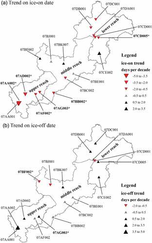
Of 17 stations, 12 revealed trends towards earlier ice-on dates, particularly in the upper and lower reaches (see Fig. 6(a)). While stations in the upper reach showed statistically significant trends (p < 0.05), only one station in the lower reach (07CD005) recorded a statistically significant trend. The two stations in the middle reach (i.e. 07BJ001 and 07BE001) displayed no changes, whereas three other stations, mostly within the middle part of the basin, showed trends towards delayed ice-on dates. However, the delayed ice-on trends were not found to be statistically significant (at p < 0.05).

Figure 6. Trends in (a) ice-on date and (b) ice-off date. The station name in bold font with * denotes statistically significant trend at the 5% significance level.

At the TFM, the analysis of historical flow and water level data revealed a shift in freeze-up timing. In earlier decades (i.e. the 1960s and 1970s), freeze-up generally occurred during the first two weeks of November, whereas in later decades (1980s–2000s) an earlier shift towards the last two weeks of October has occurred. Trend analysis showed a statistically significant decreasing rate of −0.17 day/year (p = 0.037). Not only freeze-up timing but also a decreasing trend in freeze-up stage was observed at the gauging station in the TFM (at a rate of −1.02 cm/year (p = 0.08). This also is partly explained by the decreasing patterns in air temperature and streamflow; as Prowse et al. (2007) state, a colder climate with reduced flows results in earlier freeze-up, whereas a warmer climate accompanied by increased flows contributes to delayed freeze-up. The trends for average monthly air temperature and average monthly streamflow for October for the last 52 years (1961–2012), as observed at the meteorological station Fort McMurray-A and the river gauge station at the TFM (07DA001), showed a gradual decline in both average air temperature (at a rate of −0.032°C/year) and streamflow (at a rate of −3.70 m³/s per year). However, trend analyses yielded statistically significant trends at the 5% significance level for the discharge, but not for the air temperature.

Although western Canada, in general, is reported to experience earlier breakup trends (e.g. Lacroix et al. 2005), the ice-off dates data showed most of the stations in the upper and lower reaches are recording a delay in ice disappearance (see Fig. 6(b)). However, trends at only two stations (i.e. 07AG003 and 07BF002) were found to be statistically significant (at p < 0.05). Similar to freeze-up patterns, the stations in the middle reach revealed mixed results, with two stations recording earlier trends, one station reporting a delayed trend and the remaining three stations showing no trends. Streamflow trends in these stations, in general, revealed decreasing patterns for April and May, particularly in gauges in the main stem of the river. Few tributary flows (such as at stations 07BB002 and 07CE002) showed increasing trends, but were not found to be statistically significant. Air temperatures in general for April also showed an increasing trend from 0.005°C/year at Jasper East Gate in the upper reach to 0.044°C/year at Fort McMurray-A in the lower reach.

At the TFM, 95% of the breakup events between 1958 and 2014 occurred from mid-April to mid-May. The trend analysis of breakup dates showed no sign of earlier breakup or any statistically significant change in breakup dates. However, declines in average monthly flows in April and May for the period 1958–2012 were observed. For instance, the average monthly flow in April and May at the gauging station 07DA001 at the TFM was at a decreasing rate of −2.48 and −4.7 m³/s per year, respectively. However, at the 5% significance level, the trends were not found to be statistically significant.

3.2 Calibration and validation of RIVICE

Figure 7(a) shows the model calibration result for the 1979 ice-jam flood event. It demonstrates good agreement between the surveyed and simulated water level profiles. The diamond (red) shapes show observed ice-induced water levels, which is in good agreement with the simulated ice cover. The observed measurements are available across 19 locations along the simulated reach. The comparison of performance of simulated water levels at these 19 observed locations showed a NS value of 0.89, R² of 0.93, MAE of 0.37 m and RMSE of 0.44 m. However, there are also some biases at some locations. The largest error, of about 1 m, is at chainage 8932, which translates to about 10% error. However, the statistical analyses show that the average error for all simulated locations is only 4.5%.

Figure 7. Longitudinal profiles of simulated and observed water levels along the Athabasca River from Mountain Rapids to near Shipyard Lake: (a) calibration of 1979 ice-jam flood event and (b) validation of 1977 ice-jam flood event. At the figures’ top, indicated locations are: (i) Clearwater river confluence and (ii) WSC station, Athabasca River below McMurray.

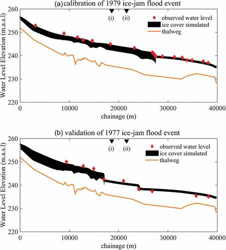
Figure 7(b) shows the results from the validation on the 1977 ice-jam flood event. The ice cover simulation results correspond well with the ice-induced water level observations. However, also in validation, there are some errors between simulated and observed water levels at some locations. The largest difference appears around chainage 17000, but this could be also due to uncertainty in the measured data, as well as how values are compared with respect to chainage location. Sometimes measured data are not available at the exact cross-section location. So when values are compared with the nearest cross-section, there can be marked differences. For instance, at chainage 17000, the simulated water level for the 1977 event is 244.684 m a.s.l. and at chainage 17100, it is 242.315 m a.s.l. That is a difference of 2.369 m. The observed value lies between chainage 17000 and 17100; hence, the error can increase or decrease based on which chainage the observed water level is being compared to. Nevertheless, a NS of 0.70, R² of 0.76, MAE of 1.17 m and RMSE of 1.26 m were achieved in the validation.

3.3 Discharge thresholds for overbank flow

Of the 1000 MOCA ice-jam simulations, 389 cases of overbank flow were simulated when the water level profile was higher than any point along the river bank profile for the TFM, as shown in Fig. 8. Then the distribution of the upstream discharge (which is a combination of both the Athabasca and Clearwater rivers) was analysed to determine the magnitude of discharge required to result in overbank flow. The probability was calculated based on the number of times a discharge value resulted in overbank flow. The resulting probability distribution (see Fig. 9) shows that, at different discharge magnitudes, various probabilities of overbank flow can be expected. For a 50% probability of overbank flooding, the results show that a discharge >1000 m³/s is required. As discharge increases, the probability further increases, leading to higher chances of overbank flow. The finding is also in line with previous observed ice-jam flooding events in the ARB. During the 1957–2012 period, there were 14 cases of ice-jam flooding recorded and, in all of those cases, breakup flows were higher than 1000 m³/s (Rokaya 2018). However, it is to be noted that it is not the probability of an ice jam occurring in any one year that is of interest, but rather the probability of backwater elevation based on upstream discharge. Occasionally, backwater staging can also result from under-developed ice jams or covers from remnants of fragmented ice.

Figure 8. Longitudinal profiles of 1000 simulated water levels along the Athabasca River (different coloured lines show the ensemble).

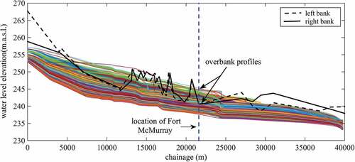
Figure 9. Probability of overbank flow of the river at different discharges.

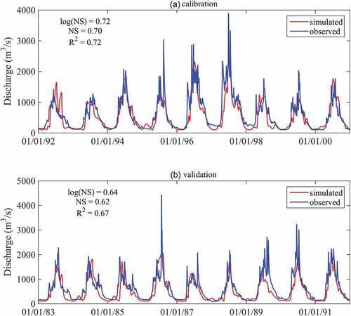
3.4 Hydrological model performance

Figure 10 shows the results from the calibration and validation at a daily time scale. Values of logNS of 0.72, NS of 0.70 and R² of 0.72 were achieved for the calibration period, whereas logNS of 0.64, NS of 0.62 and R² of 0.67 were obtained for the validation years. The average performance of the model can be attributed to two different sources of uncertainty. Firstly, the ARB is characterized by both climatic diversity and spatial variability in the hydrological processes, due to its physiographic heterogeneity. Modelling large-scale northern basins still remains a great challenge due to limited data, over-parameterization of the models, the complexity of snow processes that are difficult to capture numerically and the intricate interactions between the atmosphere and land surfaces. Previous studies in the ARB have also only been able to achieve satisfactory results. Leong and Donner (2015) reported a NS of 0.35 over an entire 30-year time period (1981–2010), with the best results achieved in the 1991–2000 decade (NS = 0.72) and the most underestimated in the following 2001–2010 decade (NS = −0.68), using the land surface process model Integrated BIosphere Simulator (IBIS), which is similar to MESH. Eum et al. (2014) were able to achieve NS values from 0.61 to 0.87 during the calibration period of 1983–1988 and from 0.56 to 0.82 (during the validation period of 1989–2010 at a monthly scale across different stations in the ARB, using high-resolution gridded climate datasets with the distributed and process-based hydrologic model, Variable Infiltration Capacity (VIC). Similar, good agreement (NS = 0.72) was reported by Toth et al. (2006), on a monthly time scale, using the distributed hydrological model WATFLOOD and station-observed meteorological data. However, on a monthly time scale, errors are averaged out by removing spikes, which results in improved statistical performance.

Figure 10. Daily observed and simulated discharge at the TFM (07DA00) for the calibration and the validation periods.

Secondly, some processes and their interactions, such as land cover changes and human interventions, are not adequately represented in some hydrological models. The Alberta oil sands, the third largest crude oil reserve in the world, also uses water from the Athabasca River, which is presently allocated at 4.4% of the mean annual flow. This study did not consider this industrial water withdrawal, which may have some consequences on river ice processes and downstream ecology. For instance, Andrishak and Hicks (2011) found that industrial water withdrawal had some impacts on winter flow affecting fish habitat in the downstream Fletcher Channel. Nevertheless, unlike previous hydrological studies in the ARB, this study simulated historical and future conditions using a physically-based land-surface hydrological model at a very high temporal resolution using 3-hourly meteorological forcing data, accounting for both energy and water balances.

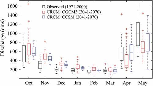
3.5 Future flow conditions

The hydrological simulation of future flow conditions is presented in Fig. 11. It shows that, compared to the historical baseline period, winter flows are expected to be higher, especially between November and January. CRCM+CGCM3 shows an average increase of ~30% in streamflow between November and January, whereas CRCM+CCSM projects an ~25% increase on an average over the same months. CRCM+CGCM3 also reveals higher variability and slightly larger mean flows in February and March compared to the historical period. However, CRCM+CCSM does not display any discernable patterns for February and March. Flows in late spring, especially in May are projected to decrease. CRCM+CGCM3 shows a substantial decrease (~45%) with respect to CRCM+CCSM, which reports a comparatively modest decrease (~25%) in comparison to historical baseline flows. The difference between two AOGCMs may be related to equilibrium climate sensitivities and how boundary conditions are defined, or whether any coupling/adjustment was carried out (Randall et al. 2007).

Figure 11. Average monthly historical flows (1971–2000 period) and the model simulation of future flows (2041–2070) at the TFM (07DA001). The box plots illustrate the median and inter-quartile range and the upper and lower limits of the whiskers from two different AOGCMs.

However, these results of increased winter flows and decreased late spring flows are not surprising, but rather expected for two reasons. First, an increase in rainfall events and a decrease in snowfall events in the Athabasca watershed is anticipated due to the warming climate (Dibike et al. 2018b). Second, more snowmelt runoff will occur in winter depleting the snow cover available for melting in the late spring months of April and May (Dibike et al. 2018a). A study by Leong and Donner (2015) in the ARB also found that, though winter flows might increase, spring/summer flows will significantly decrease in the future. A study by Erler et al. (2015) using dynamically downscaled climate projections also suggested similar results. Spring flows are driven by snowmelt and a recent study by Dibike et al. (2018a) indicates that the snow water equivalent might decrease by as much as 50% by March and April at the end of the century.

4 Discussion

4.1 Ice phenology in the Athabasca River

Our results show general trends towards earlier ice-on dates and later ice-off dates in the upper and lower reaches of the ARB, but mixed trends in the middle reach. The earlier ice-on trends and later ice-off trends, especially in tributary rivers, are in contrast to what is expected in warming cold regions. Previous studies of river and lake ice in Canada (e.g. Zhang et al. 2001, Lacroix et al. 2005, Duguay et al. 2006) have found no discernible trends in freeze-up but earlier breakup trends in western Canada. However, de Rham et al. (2008) studied the temporal variations in river-ice breakup in the Mackenzie basin, which encompasses the ARB. While they found the majority of the stations showing early breakup trends, they also report that the Athabasca River at Fort McMurray gauge readings show no trend of earlier initiation of breakup, similar to our findings.

These earlier ice appearances may be associated with atmospheric and hydrological conditions, since, from an energy balance perspective, the rate of autumn water-to-atmosphere cooling and the summer heat budget govern initial ice development and subsequent freezing (Prowse 1995). While our trend analyses for streamflow showed decreasing trends for October across all stations, air temperature trends for October have been spatially inconsistent across the basin. The meteorological stations in the upper reach (Jasper, −0.023°C/year and Jasper East Gate, −0.024°C/year) and lower reach (Fort McMurray-A, −0.032°C/year) revealed decreasing trends, while those in the middle reach (Sion, 0.021°C/year; Campsie, −0.028°C/year; Athabasca, 0.009°C/year) showed mixed results. However, spatial air temperature patterns are in correspondence with ice-on dates across the basin, since decreasing October air temperatures are reported for the upper and lower reaches, showing earlier ice-on dates, and the middle reach, with mixed air temperature trends, is showing varying patterns of ice-on dates. Ginzburg (1992) also found correlations (R² = 0.6–0.7) between freeze-up date and mean air temperature of the preceding autumn.

Our results show spatially inconsistent ice-on and ice-off patterns across the basin highlighting the complexity of ice formation and breakup processes, which are not spatially contiguous. Theoretically, it is expected that the ice cover in the Athabasca River will initiate at a bridging, for instance at the basin outlet in the northern reach, and then extend towards the headwater in the southern reach by juxtapositioning of frazil ice that is generated in upstream open-water stretches. However, due to distinct geomorphological features (e.g. sharp meanders and width constrictions) and physical barriers (e.g. bridge piers, islands and bars), bridgings can occur simultaneously at several locations along the river during the freezing period. Similarly, ice-cover breakup, although expected to occur first in the upstream southern reach and then gradually progress towards the downstream northern reach, can also happen simultaneously at several locations. But most freeze-up/breakup studies are carried out at a continental or regional scale, and generally an average trend of many stations or a trend result from only a major mainstem station (usually at the basin outlet) is reported; thus, they are likely to misrepresent local patterns, especially in tributary channels. Therefore, contrary to general reporting of earlier breakup trends in western Canada, only three stations in the ARB show earlier ice-off dates.

4.2 Significance of discharge in ice-jam flooding

Climatic and hydrological conditions, along with channel morphology and ice characteristics, influence the timing and impact severity of river ice at freeze-up and breakup. From the perspective of ice-jam flooding, spring flows play an important role. Previous studies (e.g. Beltaos 2003, Beltaos and Carter 2009, Rokaya et al. 2018b) have found that, among other hydro-meteorological conditions, freeze-up stage and breakup flow play larger roles in ice-jam flooding. Thus, with all other factors being equal, the probability and magnitude of IJFs are higher if the freeze-up stage during ice-cover formation is lower, and spring flow during ice-cover breakup is higher (Beltaos 1997).

Our stochastic river ice analyses show that, a discharge of at least >1000 m³/s is required to have a 50% probability of overbank flow along the Athabasca River at Fort McMurray. This threshold, along with the derivation of a discharge–overbank flow probability curve, can serve as an important benchmark for future river ice studies. A similar study was carried out by Beltaos (2003) for the Peace River, using a trial-and-error method and establishing a discharge of 4000 m³/s as a minimum threshold flow for ice-jam flooding. But, as shown in Fig. 2, while open water discharge and water levels can be associated with a smooth deterministic curve, backwater levels from ice accumulations or the more severe ice jam events cannot be due to the stochastic nature of river ice processes. The stochasticity in the discharge–water level relationship stems from the fact that similar backwater level profiles can occur through different water and ice flow conditions leading to ice jamming. Our method is an improvement, since it does not rely on a single trial-and-error simulation, but adopts an ensemble of possible ice-jam flooding scenarios from which the probabilities of potential ice-jam flooding discharge can be drawn.

Ice-jam flood studies for future conditions require complex hydraulic simulations for which a large number of parameters and boundary conditions will be necessary. Due to data limitations, large uncertainties and modelling challenges, future ice-jam flood studies are limited at present. Although our probability curve cannot estimate future ice-jam conditions, it is still useful to relate future flow conditions (that can be derived with hydrological models) to the probability of overbank flow.

4.3 Probability of IJFs in future

Projected future decreases from south to north air-temperature gradients suggest that the severity of ice-jam flooding may be reduced, but this could be mitigated by changes in the magnitude of spring snowmelt (Prowse et al. 2011). A study by Das et al. (2017), using the cumulative degree days of melting and cumulative degree days of freezing approaches on future meteorological data from NARCCAP, found that the average freeze-up in the future will begin from the third week of October and the average breakup will occur in April for the TFM. Our simulation of future hydrological conditions (2041–2070 period) reveals that median flows in April will be lower by about 50% compared to the historical baseline period of 1971–2000. Similarly, median November flows are projected to increase from 20% (CRCM+CCSM) to 30% (CRCM+CGCM3) compared to the baseline historical period. Higher flows in autumn can lead to higher freeze-up stage in rivers. From the perspective of ice-jam flooding, the probability and magnitude of IJFs are lower if the freeze-up stage during ice-cover formation is higher, and spring flow during ice-cover breakup is lower. Since our results show higher flows in November and reduced spring flows in April, the probability of IJFs of the TFM may be lower in the future. In their study of the neighbouring Peace River basin, Prowse et al. (2007) also state that a decreasing flow pattern can reduce the likelihood of dynamic breakup and ice-jam flooding events, as higher spring flows are required for dynamic breakup and subsequent flooding events. However, caution is advised in interpreting these results. Mechanical breakup events that lead to severe IJFs are driven by peak instantaneous/daily flows and, though average monthly flow is projected to be lower, extreme daily flow events are still probable. This is particularly plausible, since, in spite of lower median April flows, the whisker shows a large variability including large upper quartile and extreme values, especially for CRCM+CCSM (see Fig. 11). Thus, although the probability of IJFs in general is expected to be lower for the TFM, extreme IJF events including mid-winter breakups can still occur under favourable hydro-meteorological conditions.

5 Conclusion and future recommendation

This study demonstrates significant hydro-climatic variability in the Athabasca River basin, which has implications for river ice processes. The analysis of ice-on and ice-off dates revealed a spatially inconsistent pattern across the basin, highlighting that ice formation and breakup processes are complex and spatially non-contiguous. However, ice-on and ice-off dates showed a high correlation with air temperature. River ice MOCA simulations showed that, for a 50% probability of overbank flow at the TFM, a discharge of at least 1000 m³/s is required. Deriving flow thresholds for IJFs using a probabilistic method that incorporates stochasticity of river ice processes is a novel approach, and can serve as an important benchmark for future river ice studies, especially for estimating future IJF probabilities. This approach can be extended to other ice-jam prone northern rivers to understand the relative role of discharge in IJFs.

The analyses of future flow conditions based on both RCMs and AOGCMS showed that, while average winter flows may increase by ~25%, the late spring flows may reduce by about 50% in the 2041–2070 future period compared to the historical baseline period of 1971–2000. The increased freeze-up flow and decreased breakup flows suggest that the probability and magnitude of IJFs in the future may be lower for the TFM; nevertheless, extreme IJF events are still probable. Further assessments are needed to quantify future ice-jam flood risk. More research is required to couple hydrological and hydraulic models so that hydrological models can provide important boundary conditions for hydraulic models to simulate future river ice conditions. Such coupled model configurations should also incorporate other important climate factors, such as air temperature and precipitation. In ice-jam prone cold region environments, future IJF risk assessments and hazard mapping are essential to assist in making proper land-use plans and designing risk-alleviating hydraulic structures and other mitigation measures.

Acknowledgements

The authors are thankful to Mr Dennis Lazowski with WSC Alberta for water levels and ice thickness data, Prof. Faye Hicks for the Athabasca cross-section data, Mr Daniel Princz and Dr Gonzalo Sapriza-Azuri for their assistance with MESH and Mr Hammad Javaid for his support in NARCCAP data processing. The editor, two anonymous reviewers and Dr Daniel Peters provided constructive feedback that helped to improve this manuscript.

Disclosure statement

No potential conflict of interest was reported by the authors.

Additional information

Funding

This work is supported by the Canadian Excellence Research Chair in Water Security through the Global Institute for Water Security, University of Saskatchewan.

Notes

¹ https://ec.gc.ca/rhc-wsc/default.asp?lang=En&n=9018B5EC-1.

² http://climate.weather.gc.ca/.

References

- Andres, D.D. and Doyle, P.F., 1984. Analysis of breakup and ice jams on the Athabasca River at Fort McMurray, Alberta. Canadian Journal of Civil Engineering, 11 (3), 444–458. doi:10.1139/l84-065
- Andrishak, R. and Hicks, F., 2011. Ice effects on flow distributions within the Athabasca Delta, Canada. River Research and Applications, 27 (9), 1149–1158. doi:10.1002/rra.1414
- Bawden, A.J., et al., 2014. A spatiotemporal analysis of hydrological trends and variability in the Athabasca River region, Canada. Journal of Hydrology, 509, 333–342. doi:10.1016/j.jhydrol.2013.11.051
- Beltaos, S., 1997. Onset of river ice breakup. Cold Regions Science and Technology, 25 (3), 183–196. doi:10.1016/S0165-232X(96)00011-0
- Beltaos, S., 2003. Numerical modelling of ice‐jam flooding on the Peace–Athabasca delta. Hydrological Processes, 17 (18), 3685–3702. doi:10.1002/(ISSN)1099-1085
- Beltaos, S., 2018. The 2014 ice–jam flood of the Peace-Athabasca Delta: insights from numerical modelling. Cold Regions Science and Technology, 155, 367–380. doi:10.1016/j.coldregions.2018.08.009
- Beltaos, S. and Burrell, B.C., 2003. Climatic change and river ice breakup. Canadian Journal of Civil Engineering, 30 (1), 145–155. doi:10.1139/l02-042
- Beltaos, S. and Carter, T., 2009. Field studies of ice breakup and jamming in lower Peace River, Canada. Cold Regions Science and Technology, 56 (2–3), 102–114. doi:10.1016/j.coldregions.2008.11.002
- Beltaos, S. and Prowse, T.D., 2001. Climate impacts on extreme ice-jam events in Canadian rivers. Hydrological Sciences Journal, 46 (1), 157–181. doi:10.1080/02626660109492807
- Burn, D.H., Abdul Aziz, O.I., and Pietroniro, A., 2004. A comparison of trends in hydrological variables for two watersheds in the Mackenzie River Basin. Canadian Water Resources Journal/Revue Canadienne Des Ressources Hydriques, 29 (4), 283–298. doi:10.4296/cwrj283
- Canadian Hydraulics Centre, 2010. Green kenue reference manual. Ottawa, Ont: National Research Council Canada.
- Caya, D. and Laprise, R., 1999. A semi-implicit semi-Lagrangian regional climate model: the Canadian RCM. Monthly Weather Review, 127 (3), 341–362. doi:10.1175/1520-0493(1999)127<0341:ASISLR>2.0.CO;2
- Das, A., Rokaya, P., and Lindenschmidt, K.-E., 2017. Assessing the impacts of climate change on ice jams along the Athabasca River at Fort McMurray, Alberta, Canada. In: Proceedings of 19th workshop on the Hydraulics of Ice Covered Rivers, Whitehorse, Yukon, Canada.
- de Rham, L.P., Prowse, T.D., and Bonsal, B.R., 2008. Temporal variations in river-ice break-up over the Mackenzie River Basin, Canada. Journal of Hydrology, 349 (3), 441–454. doi:10.1016/j.jhydrol.2007.11.018
- DeBeer, C.M., et al., 2016. Recent climatic, cryospheric, and hydrological changes over the interior of western Canada: a review and synthesis. Hydrology and Earth System Sciences, 20 (4), 1573. doi:10.5194/hess-20-1573-2016
- Déry, S.J., et al., 2011. Interannual variability and interdecadal trends in Hudson Bay streamflow. Journal of Marine Systems, 88 (3), 341–351. doi:10.1016/j.jmarsys.2010.12.002
- Dibike, Y., Eum, H.-I., and Prowse, T., 2018a. Modelling the Athabasca watershed snow response to a changing climate. Journal of Hydrology: Regional Studies, 15, 134–148.
- Dibike, Y., et al., 2018b. Effects of projected climate on the hydrodynamic and sediment transport regime of the lower Athabasca River in Alberta, Canada. River Research and Applications, 34, 417–429. doi:10.1002/rra.v34.5
- Doherty, J., 1994. PEST: a unique computer program for model-independent parameter optimisation. Water Down Under 94: Groundwater/Surface Hydrology Common Interest Papers; Preprints of Papers, 551.
- Doyle, P.F., 1977. Hydrologic and hydraulic characteristics of the Athabasca River from Fort McMurray to Embarras. Edmonton, Alberta: Research Council of Alberta, Transportation and Surface Water Engineering Division.
- Duguay, C.R., et al., 2006. Recent trends in Canadian lake ice cover. Hydrological Processes, 20 (4), 781–801. doi:10.1002/(ISSN)1099-1085
- Environment and Climate Change Canada, 2013. RIVICE model - user’s manual. Available from: http://giws.usask.ca/rivice/Manual/RIVICE_Manual_2013-01-11.pdf [Accessed 24 Jan 2017].
- Erler, A.R., Peltier, W.R., and d’Orgeville, M., 2015. Dynamically downscaled high-resolution hydroclimate projections for western Canada. Journal of Climate, 28 (2), 423–450. doi:10.1175/JCLI-D-14-00174.1
- Eum, H.-I., Dibike, Y., and Prowse, T., 2017. Climate-induced alteration of hydrologic indicators in the Athabasca River Basin, Alberta, Canada. Journal of Hydrology, 544, 327–342. doi:10.1016/j.jhydrol.2016.11.034
- Eum, H.I., et al., 2014. Inter‐comparison of high‐resolution gridded climate data sets and their implication on hydrological model simulation over the Athabasca Watershed, Canada. Hydrological Processes, 28 (14), 4250–4271. doi:10.1002/hyp.10236
- Ginzburg, B., 1992. Secular changes in dates of ice formation on rivers and relationship with climate change. Russian Meteorology and Hydrology, 12, 57–64.
- Hutchison, T.K. and Hicks, F., 2007. Observations of ice jam release waves on the Athabasca River near Fort McMurray, Alberta. Canadian Journal of Civil Engineering, 34 (4), 473–484. doi:10.1139/l06-144
- Intergovernmental Panel On Climate Change, 2007. Climate change 2007: the physical science basis. Agenda, 6 (07), 333.
- Kerkhoven, E. and Gan, T.Y., 2011. Differences and sensitivities in potential hydrologic impact of climate change to regional-scale Athabasca and Fraser River basins of the leeward and windward sides of the Canadian Rocky Mountains respectively. Climatic Change, 106 (4), 583–607. doi:10.1007/s10584-010-9958-7
- Kouwen, N., et al., 1993. Grouped response units for distributed hydrologic modeling. Journal of Water Resources Planning and Management, 119 (3), 289–305. doi:10.1061/(ASCE)0733-9496(1993)119:3(289)
- Lacroix, M., et al., 2005. River ice trends in Canada. In: 13th workshop on the hydraulics of ice covered rivers. Hanover, New Hampshire.
- Leong, D.N. and Donner, S.D., 2015. Climate change impacts on streamflow availability for the Athabasca oil sands. Climatic Change, 133 (4), 651–663. doi:10.1007/s10584-015-1479-y
- Lindenschmidt, K.-E., 2017. RIVICE—a non-proprietary, open-source, one-dimensional river-ice model. Water, 9 (5), 314. doi:10.3390/w9050314
- Lindenschmidt, K.-E. and Chun, K.P., 2013. Evaluating the impact of fluvial geomorphology on river ice cover formation based on a global sensitivity analysis of a river ice model. Canadian Journal of Civil Engineering, 40 (7), 623–632. doi:10.1139/cjce-2012-0274
- Lindenschmidt, K.E., et al., 2016. Ice jam flood risk assessment and mapping. Hydrological Processes, 30, 3754–3769. doi:10.1002/hyp.v30.21
- Mahabir, C., et al., 2006. Forecasting breakup water levels at Fort McMurray, Alberta, using multiple linear regression. Canadian Journal of Civil Engineering, 33 (9), 1227–1238. doi:10.1139/l06-067
- Mann, H.B., 1945. Nonparametric tests against trend. Econometrica, 13 (3), 245–259. doi:10.2307/1907187
- Matott, L.S., 2005. OSTRICH: an optimization software tool; documentation and user’s guide. Available from: http://www.eng.buffalo.edu/~lsmatott/Ostrich/OstrichMain.html [Accessed 11 Mar 2017].
- Mearns, L.O., et al., 2012. The North American regional climate change assessment program: overview of phase I results. Bulletin of the American Meteorological Society, 93 (9), 1337–1362. doi:10.1175/BAMS-D-11-00223.1
- Mearns, L.O., et al., 2009. A regional climate change assessment program for North America. Eos, 90 (36), 311. doi:10.1029/2009EO360002
- Monk, W.A., Peters, D.L., and Baird, D.J., 2012. Assessment of ecologically relevant hydrological variables influencing a cold‐region river and its delta: the Athabasca River and the Peace–Athabasca Delta, northwestern Canada. Hydrological Processes, 26 (12), 1827–1839. doi:10.1002/hyp.9307
- Morales-Marín, L.A., et al., 2019. A hydrological and water temperature modelling framework to simulate the timing of river freeze-up and ice-cover breakup in large-scale catchments. Environmental Modelling & Software, 114, 49–63. doi:10.1016/j.envsoft.2019.01.009
- NARCCAP, 2016. The A2 emissions scenario. Available from: http://www.narccap.ucar.edu/about/emissions.html [Accessed 8 July 2016].
- Peters, D.L., et al., 2013. A multi‐scale hydroclimatic analysis of runoff generation in the Athabasca River, western Canada. Hydrological Processes, 27 (13), 1915–1934. doi:10.1002/hyp.v27.13
- Peters, D.L. and Prowse, T.D., 2006. Generation of streamflow to seasonal high waters in a freshwater delta, northwestern Canada. Hydrological Processes, 20 (19), 4173–4196. doi:10.1002/(ISSN)1099-1085
- Pietroniro, A., et al., 2007. Development of the MESH modelling system for hydrological ensemble forecasting of the Laurentian Great Lakes at the regional scale. Hydrology and Earth System Sciences, 11 (4), 1279–1294. doi:10.5194/hess-11-1279-2007
- Pietroniro, A. and Soulis, E., 2003. A hydrology modelling framework for the Mackenzie GEWEX programme. Hydrological Processes, 17 (3), 673–676. doi:10.1002/(ISSN)1099-1085
- Prowse, T.D, 1995. River ice processes. Chapter 2. In: S. Beltaos, ed. River ice Jams. Highlands Ranch, Colorado: Water Resources Publications, LLC, 29–70.
- Prowse, T., et al., 2011. Past and future changes in Arctic lake and river ice. AMBIO: a Journal of the Human Environment, 40 (sup 1), 53–62. doi:10.1007/s13280-011-0216-7
- Prowse, T.D., et al., 2007. River-ice break-up/freeze-up: a review of climatic drivers, historical trends and future predictions. Annals of Glaciology, 46 (1), 443–451. doi:10.3189/172756407782871431
- Randall, D.A, et al., 2007. Cilmate models and their evaluation. Climate change 2007: The physical science basis contribution of working group I to the fourth assessment report of the intergovernmental panel on climate change. Cambridge, UK: Cambridge University Press, 589–662.
- Rokaya, P., 2018. Impacts of climate and regulation on ice-jam flooding of northern rivers and their inland deltas. Doctoral Dissertation. University of Saskatchewan, Saskatoon, Canada. Available from: https://harvest.usask.ca/handle/10388/9207
- Rokaya, P., Budhathoki, S., and Lindenschmidt, K.-E., 2018a. Trends in the timing and magnitude of ice-jam floods in Canada. Scientific Reports, 8 (1), 5834. doi:10.1038/s41598-018-24057-z
- Rokaya, P., et al., 2019. Modelling the effects of climate and flow regulation on ice-affected backwater staging in a large northern river. River Research and Applications. doi:10.1002/rra.3436
- Rokaya, P., Wheater, H., and Lindenschmidt, K.-E., 2018b. Promoting sustainable ice-jam flood management along the Peace River and Peace-Athabasca Delta. Journal of Water Resources Planning and Management, 145 (1), 04018085. doi:10.1061/(ASCE)WR.1943-5452.0001021
- Rood, S.B., Stupple, G.W., and Gill, K.M., 2015. Century‐long records reveal slight, ecoregion‐localized changes in Athabasca River flows. Hydrological Processes, 29 (5), 805–816. doi:10.1002/hyp.v29.5
- She, Y., et al., 2009. Athabasca River ice jam formation and release events in 2006 and 2007. Cold Regions Science and Technology, 55 (2), 249–261. doi:10.1016/j.coldregions.2008.02.004
- Sheikholeslami, R., et al., 2017. Improved understanding of river ice processes using global sensitivity analysis approaches. Journal of Hydrologic Engineering, 22 (11), 04017048. doi:10.1061/(ASCE)HE.1943-5584.0001574
- Shrestha, R.R., Schnorbus, M.A., and Peters, D.L., 2016. Assessment of a hydrologic model’s reliability in simulating flow regime alterations in a changing climate. Hydrological Processes, 30 (15), 2628–2643. doi:10.1002/hyp.10812
- Sun, W. and Trevor, B., 2018. Multiple model combination methods for annual maximum water level prediction during river ice breakup. Hydrological Processes, 32 (3), 421–435. doi:10.1002/hyp.v32.3
- Thompson, S.A., 1999. Hydrology for water management. London: CRC Press.
- Tolson, B.A. and Shoemaker, C.A., 2007. Dynamically dimensioned search algorithm for computationally efficient watershed model calibration. Water Resources Research, 43 (1), W01413. doi:10.1029/2005WR004723
- Toth, B., et al., 2006. Modelling climate change impacts in the Peace and Athabasca catchment and delta: I—hydrological model application. Hydrological Processes, 20 (19), 4197–4214. doi:10.1002/(ISSN)1099-1085
- Weller, G.B., et al., 2013. Two case studies on NARCCAP precipitation extremes. Journal of Geophysical Research: Atmospheres, 118 (18), 10,475–10,489.
- Yue, S., et al., 2002. The influence of autocorrelation on the ability to detect trend in hydrological series. Hydrological Processes, 16 (9), 1807–1829. doi:10.1002/(ISSN)1099-1085
- Zhang, X., et al., 2001. Trends in Canadian streamflow. Water Resources Research, 37 (4), 987–998. doi:10.1029/2000WR900357
- Zhang, X., et al., 2000. Temperature and precipitation trends in Canada during the 20th century. Atmosphere-Ocean, 38 (3), 395–429. doi:10.1080/07055900.2000.9649654