Internet-based applications for interrogating 50 years of data from the South African national water quality monitoring network

ABSTRACT

National and regional water quality monitoring networks have been operated in South Africa since the early 1970s. These originally had text-based inventories that were convenient for specialists who were familiar with the national networks and knew the locations of their sites of interest. However, within two decades the networks had expanded in geographical extent and variables monitored to such an extent that users needed spatial context in order to locate sites that fitted their information requirements. Mapping applications running on the Internet, such as Google Earth and Leaflet, form the foundation of a system for providing online inventories and summaries of the data available on the water quality database. The interfaces were constructed using available software, mainly ArcInfo and R. A recent concern is a decrease in the collection of water quality data, which is reducing the value of data summaries for water resource management.

KEYWORDS:

• water quality
• monitoring
• keyhole markup language (KML)
• information visualization
• data analysis
• water database
• historical records

Editor A. CastellarinGuest editor S. Uhlenbrook

1 Introduction

Nearly half of South Africa receives less than 400 mm rainfall per year (Schulze and Lynch 2006). The total runoff volume is a little less than 50 × 10⁶ m³/year (Bailey and Pitman 2015), equivalent to a mean annual runoff of 40 mm. Potential evaporation rates exceed 2000 mm in parts of the north and west (Schulze and Maharaj 2006). Under this hydrological regime, survival and development depend on detailed knowledge of water: Where is it? How much is there? Is it safe to use? These questions are as important for a nomadic hunter or subsistence farmer as they are for an industry manager or a water supply engineer. During the 20th century, the first two questions – “where?” and “how much?” – drove the development of a national hydrological monitoring network by successive national government departments of water. The third question, “Is it safe to use?” became even more important after industrial development began making its mark on river and impoundment water quality during the 1950s (Ashton et al. 2012).

1.1 History of the South African water quality monitoring networks

In the early 1970s, the Division of Hydrology in the Department of Water Affairs (now the Department of Water and Sanitation, DWS) issued a technical note in response to the SCOPE report on global environmental monitoring (SCOPE 1971), stating that:

Environmental pollution has become an international problem. However, trends in the effects of this pollution and advance warning of the approach of dangerous and possibly i[r]reversible situations, will have to be based on a sound national monitoring programme. It is in our own interest, as well as being an international obligation, that we should establish this as soon as possible. (Alexander 1972)

The first South African water quality monitoring network focused on about 15 inorganic chemical variables, making use of the existing hydrological monitoring infrastructure. At that time, most gauging stations had recorders that staff visited regularly to change the paper charts and to carry out maintenance. They simply added the collection of a grab sample at each site to their routine.

Monitoring of water quality on a large scale only became feasible with the establishment of a water chemistry laboratory using flow injection analysis, in the mid-1970s (van Vliet 1980, van Staden and van vliet 1984, van Staden 1986). The original water quality network focused on monitoring of major ions and nutrients, and it later became known as the national chemical monitoring programme. In order to handle the increasing volume of data, an in-house laboratory information management system was written, running in FORTRAN on a Varian mini-computer. Archiving and data processing took place on a separate mainframe computer.

Monitoring for trophic status indicators began during the 1980s, later being formalized as the national eutrophication monitoring programme (DWAF 2002a). During the 1990s, the national microbial monitoring programme came into being, concentrating on known hotspots for water-borne pathogens (DWAF 2002b). Other programmes monitor toxicity, radioactivity and the status of estuaries (DWS 2019a). An extensive river ecostatus monitoring programme also exists (Strydom et al. 2006) which, because of the complexity of biomonitoring results, used a separate database developed for this type of data (Dallas et al. 2007). That database is no longer maintained and a new freshwater biodiversity information system has been released by an independent research group, the Freshwater Research Centre.¹

1.2 The need for an interactive inventory

By the 1980s, sufficient water quality data were available for catchment-wide analyses of the chemical status of rivers (van Vliet and Nell 1986). The curators of the database came to the realization that the value of the water quality data lay in their being accessible for use by people with a wide variety of specializations, especially trend analysis and modelling. Consequently, many scientific and technical reports have used data from the national database (e.g. Scherman et al. 2003, Huizenga et al. 2013, Griffin et al. 2014, DWS 2019b). At first, the database was part of the national Hydrological Information System, a flow and quality database that ran on a shared government mainframe and which was only indirectly accessible to most users. Data transfer between systems was by magnetic tape; printed catalogues listed the hydrological gauging stations, many of which were also water quality monitoring sites (DWA 1976).

By the end of the 1980s, a large amount of water chemistry data had been archived; for example, the number of orthophosphate records stored on the database had reached 237 854. In order to make sense of this volume of data, a visual catalogue was developed, listing every monitoring site, each with a bar chart showing the monitoring frequency for 17 major variables (Swart et al. 1991a). Developing this paper catalogue was a complex task, with a number of steps required for getting data from 9-track magnetic tape to 5¼″ floppy disks and from there to a personal computer, with limited storage (typically 20 Mb of disk space), where software written in Pascal generated the graphical output. The printed report comprised two yellow-bound A4 volumes, each several hundred pages long (Swart et al. 1991a, 1991b).

2 Development of an interactive inventory

2.1 Prototype

While the “yellow pages” report provided a new and unique insight into the data available, it was a static document requiring a great amount of manual effort for preparation (Swart et al. 1991a). Some form of dynamic system was required for providing up-to-date information about what results were on the database and where they were monitored.

The first interactive geographical water quality data query system developed by DWS was known as WaterMarque.² This system, operating on Unix workstation versions 6 and 7 of Esri’s ArcInfo, allowed users to make queries from a routinely-updated text file containing a subset of the laboratory water quality database. WaterMarque retrieved the selected results and presented them on maps with symbols indicating water quality status, plotted against a background of spatial data that could include vegetation type, geology, soils, climatic variables and land cover. Time series plots could also be shown alongside the map, in what would now be recognized as a dashboard layout (Cobban and Silberbauer 1993, Cobban 1994, Silberbauer 1997). Access to WaterMarque was limited to a few workstations on a local area network.

At the time that WaterMarque was first released, the Internet had begun to be generally accessible in South Africa. Developers of WaterMarque saw this as a new opportunity for distributing water quality data on demand, so they set up a simple prototype inventory using HTML on an 80486 PC running Apache server software. A set of data summary plots was developed using a cataloguing tool called BARCODE (Silberbauer 1997).The prototype was lost soon afterwards when the server succumbed to a lightning strike, but a fragmentary record survives on the Wayback Machine³ for the 1990s (Internet Archive 2019).

2.2 Keyhole markup language (KML) and Esri

In 2005, the Keyhole satellite image viewing software became publicly available as Google Earth, a 2.5D image rendering application that users can customise with an extensible markup language, KML.⁴ Its main advantages are that it can be used as a free viewing platform with user data placed in the foreground using KML code, and that the algorithm for download of background images is extremely efficient (Crampton 2008).

The first development was a simple procedure in the awk text-processing language (Aho et al. 1988) that generated KML files from a flat file containing the catalogue of monitoring sites. Procurement of licensed software is an uncertain process in government organizations, so Unix Esri ArcInfo, the only graphics software readily available on the local server, was chosen as the development platform for generating time series plots for each monitoring site, using PDF format for maximum resolution. Programming was in Arc Macro Language (AML) (Silberbauer 1997). Slow Internet speeds and network security concerns precluded any direct user interaction with the water quality database or geographical data, so the workflow consisted of pre-generating hundreds of static HTML and KML files with linked bitmap images. These files were then uploaded to the web server.

2.3 R software

By 2011, managing the Esri-based system for generating website files for water quality using the AML scripting language was becoming unwieldy and the Unix workstations were being phased out, so it was an opportune moment to select another development platform. The R open source statistics and graphics software showed promise – while development of R had already started in the 1990s, its wide distribution and popularity grew steadily in the first decade of the 21st century (Smith 2017, R Core Team 2018). After a testing phase, conversion of the awk and AML scripts to R-based processes for publishing water quality data began (Fig. 1).

Figure 1. Simplified workflow showing the processes for collecting, curating and visualizing South African water quality monitoring data.

2.3.1 Chemistry monitoring network

Using computer programs to generate markup language files in HTML and KML is a straightforward but cognitively difficult process of using code to generate code, which creates two areas for error: the code that produces the markup files and the markup files themselves. Standardizing on one platform, R, instead of combining awk and Esri scripting, simplified documentation and maintenance of this process.

Innovative R packages for spatial analysis, such as sp and maptools, facilitated static map production within the R environment⁵ (Bivand et al. 2013), obviating the need for a separate geographical information system. The RODBC package⁶ allowed direct SQL queries to the Informix-based water quality database on a Unix server, cutting out the need for regular exports from the database to intermediate text files. By 2011, R scripts were operational for KML inventories (Silberbauer 2018a) and time-series plots of water quality (Silberbauer 2018b). A guide to the use of the system is available online⁷ together with further background details.⁸

Specialized symbols were also developed in R, for example an implementation of the Maucha ionic diagram (Fig. 2). This symbol provides an instant, qualitative view of the proportions of major ions in a sample (Maucha 1932, Broch and Yake 1969, Hassel et al. 1997, Silberbauer 1997, van Niekerk et al. 2014).

Figure 2. An example of the metadata shown by clicking on a monitoring site in the Google Earth KML-based inventory. See text for explanation. The information box has been redrawn for clarity, and the original KML file is available online (http://www.dwa.gov.za/iwqs/wms/data/A_reg_WMS_nobor.kmz). Sources: Background image: Google Earth; inventory information: DWS publicly available water quality database.

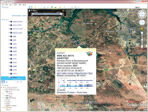
The example in Fig. 2 shows a monitoring site downstream of major point and non-point pollution sources and upstream of a water supply impoundment, Roodeplaat Dam. The underlined links take the user to further sources of information: plot – time-series plot of major chemical variables; data – comma-separated-value text file with the data used to create the time-series plot, along with detailed metadata about the site and the analytical methods; Maucha key – explanation of the symbol in the top right of the information box; flow – a link to the separate hydrological database.

2.3.2 Microbial monitoring network

Unlike the chemical monitoring programme, which developed over time, the microbial monitoring programme functions and data flow were set out in a formal implementation manual (DWAF 2002b). The unstable nature of microbial samples required that DWS appoint contracted laboratories near regional monitoring sites, so that the time from sampling until analysis could be kept under 24 hours. Furthermore, microbial events are transient, so the feedback of information to regional managers needed to be improved. The microbial programme implementation documents included spreadsheets for data entry and calculation of results in each management region. The manager of the monitoring programme was required to update the spreadsheets on a two-monthly cycle and manually distribute them to managers by email or fax. During 2011, in an effort to streamline this process, the functions of the spreadsheets were emulated in an R procedure for generating a set of HTML tables with static maps for each two-month period, available online. The current version of the microbial reporting web page is updated weekly and includes additional information, for example plots of the full microbial record of each site and KML files for viewing the sites geographically. The R code is available for download from the DWS.⁹

The microbial website now also provides access to results via an interactive Leaflet map interface, which is based on a publicly available R script, R2leaflet.R (Grant 2013). In addition, the water quality database includes many routinely collected microbial records for sites such as pollution sources that are not part of the microbial monitoring programme: these are available via a separate interface. The raw data for all monitoring locations are also available, so that advanced users can do their own analysis.

2.3.3 Eutrophication monitoring network

Routine collection and reporting of eutrophication-related data by DWS began in the 1980s (van Ginkel 2011). The programme was later formalized as the national eutrophication monitoring programme (DWAF 2002a). In 2011 an Internet reporting system for eutrophication data was prototyped. The layout for each six-monthly summer and winter period comprised a static map of the eutrophication sites, with symbols indicating their status, and a table listing details of chlorophyll a and orthophosphate at sites, with links to further information such as Secchi disc measurements, and profiles of temperature and oxygen, also generated in R.¹⁰ Proposed developments include an interactive map interface to the full eutrophication dataset: currently, a map interface to recent eutrophication data is available via the National Integrated Water Information System (NIWIS) dashboard system developed in a different branch of DWS.¹¹

3 The benefits of visual inventories

The literature on data visualization is extensive, from the physiology and pathology (Guyton and Hall 2000), the human visual processing system (Ware 2008), to symbols (Bertin), design (Tufte 2001, Lanthony 2006, Ware 2008, Few 2009) and maps (MacEachren et al. 2004, Slocum et al. 2008). Visualization of data makes use of the rapid processing capacity of the viewer’s eyes and visual cortex for transferring information that would take much longer to explain using speech and logic centres. For example, a map quickly shows that Site A is upstream of Site B, a sewage treatment works discharges effluent between the two, a village is located downstream of Site B. This happens so quickly for most people that it seems trivial, yet it rates a formal classification as the “relationships among three variables”, namely the two dimensions of the map and the single variation of marks on it (Bertin 1967, 1983, 2010). Supporting information needs to be conveyed by slower verbal means, e.g.: “the sewage works complies with microbial discharge regulations for 30% of the time; the villagers downstream use the river water for drinking and washing; take appropriate action.” Colloquially, we build up a “picture” of the situation that helps us to decide how to deal with it.

3.1 Points to note with visualization of data

Visualization requires consistent use of signs and symbols, which, for images in print or on static computer display can vary in size, value, texture, colour, orientation and shape (Bertin 2010). Inadequate resolution, ill-judged hatching or use of colour, illegible annotation: many such shortcomings will obscure the viewer’s interpretation (Tufte 2001). Standardization is required where rapid and unambiguous interpretation of symbols is important but mapping of scientific data is not consistent: for example, the Internet visualizations of South African data described in this paper have their own colour-coding and symbols, but these are more guidelines than an actual code.

Using the Internet as a medium for communication obviously requires that users are able to access the world-wide network (W3C WAI 2019), with slightly more than one in three people in Africa having Internet access in 2017, although this figure is increasing (IWS 2019). Pathologies also intervene: for example a proportion, perhaps 8%, of male viewers may have red-green colour blindness and the message of a colour-coded map or graph may be less clear to them than intended. Careful choice of colour combinations will help in this relatively common and mild condition (Olson and Brewer 1997), but what of more severe pathologies, or the lack of any vision at all? In sub-Saharan Africa, blindness and visual impairment rates have decreased, but are still higher than the global average (Naidoo et al. 2014). Often, visual impairment is refractive, in which case corrective lenses will help at relatively low cost. In the case of health effects, prevention is clearly the first step: causes include diseases such as trachoma and onchocerciasis, which are related to management of water and sanitation. Tactile interfaces such as Braille, ridged graphics and the use of sound may assist in conveying information through other senses in order to build up an internal model in the imagination of the reader, but they all depend on a correctly-formulated HTML structure (W3C WAI 2019).

4 Practical implications

Before distribution of DWS data via the Internet, users could either rely on printed reports (Swart et al. 1991a) or make direct requests to DWS for data to be sent to them in text files. Requesting data required familiarity with the alphanumerical site naming convention for monitoring sites located at hydrological structures (McDonald 1989), or the numerical “feature identifiers” used on the national water quality database.

The provision of spatial interfaces to water quality data simplified the process of choosing suitable monitoring sites for any application, because their location in relation to hydrological features, pollution sources and water users was instantly visible. Selection of sites active within a specified period was facilitated using mechanisms such as the “time slider” in Google Earth (Google Developers 2018). The instant metadata and summary available by clicking on a candidate site has further helped users in narrowing down a search for relevant information. While datasets comprising major ions, nutrients and metadata in text files are available for download, a call centre is still available for obtaining more specialized datasets, for example trace metals or organic compounds, which are not yet shown online. The “standard” way of transferring the numerical data described in this paper is via text files using the simple comma-separated-value (CSV) format. However, even CSV presents problems in locales where the decimal separator is a comma. The addition of more advanced information, such as analytical methods, units and limits of detection is more complicated, especially when these are taken out of the environment of a relational database. The metadata text files included with the CSV data files are an imperfect solution: More advanced methods developed elsewhere rely on data interchange structures in extensible markup language (XML) that permit the inclusion of contextual information. Notable examples are the USA Water Quality Exchange (WQX)¹² and the Open Geospatial Consortium (OGC) WaterML 2.0 standard.¹³ The focus of the latter is currently on flow gauging data. Reaching consensus on representing complex water quality datasets is a difficult process, so this is an important area for development.

An unexpected advantage of wide distribution of the water quality information became evident to the curators of the data. With many eyes on the database, problems that DWS staff had not yet picked up began to be reported by external users: the most common were coordinate errors. With more than 65 000 sites, many established in the days of paper maps, errors in location were perhaps inevitable, and have been fairly straightforward to correct in those cases where good descriptive information is available. A more serious problem identified by users was a systematic error in pH results from samples collected in the 1980s, where the analytical method had resulted in lower pH values, especially in poorly-buffered samples (Ramjukadh et al. 2018).

An inventory reflects available stock. With increasing costs and a budget that has not kept pace with monitoring requirements, the ability to comply with sampling frequencies has gradually declined since 2010, reaching a low point in late 2018 (Fig. 3). In the middle of that year, almost all water quality monitoring was put on hold when the DWS analytical laboratories suspended operations because of insufficient funding, a situation that is expected to continue for much of 2019. Monitoring that still occurs is limited to that carried out by municipalities and water supply entities, whose focus is on urban areas and pollution sources rather than ambient water quality. In 2017, South Africa was able to submit a comprehensive baseline report for sustainable development goal SDG 6.3.2 (UNEP 2018), but the resumption of national monitoring will be necessary before South Africa can report on future progress with achieving the targets of this goal.

Figure 3. The South African water quality monitoring rate represented by the number of orthophosphate analyses recorded per year. Dips in production in 1979, 1983 and 2010 were related to movement or renovation of laboratories, while the decrease in 2018 came after cuts in expenditure. Source: Department of Water and Sanitation publicly available water quality database.

5 Is this a model for system development?

The development of the Internet-based reporting systems described here occurred in response to user requests for data, modified by circumstances such as skills and technology available. It was not part of a grand information technology plan, and did not have access to special funding. Therefore, it had to rely on software that was already available or software that did not have a licence fee. When development started in the early 1990s, hydrological software focused on storage of time series data from flow gauging stations, as implemented in the in-house Hydrological Information System and Hydstra.¹⁴ Since then, commercial hydrological software has expanded to include water quality indicators, for example the water quality applications in Hydstra and Aquarius.¹⁵ Off-the-shelf solutions such as these, which combine data storage and information visualization, may be a better choice for organizations that have a budget for licence fees. In this regard, note that the in-house development described in this paper is purely on the reporting side, and the development of the locally-designed Informix water quality database took place in a separate IT section with dedicated resources.

The in-house development of reporting methods has certain advantages if the right skills are available, which include programming in a language such as R or Python combined with experience in water quality data interpretation and an understanding of what data users require. In-house development is flexible and can respond to changing user requirements. A disadvantage of in-house development is that in order to be sustainable it requires an environment that includes succession planning for skills transfer and that encourages creativity. One way to ensure the survival of a set of systems designed in R is to combine the components into an R “package”, such as smwrGraphs developed at the US Geological Survey (Lorenz and Diekoff 2017) and make it publicly available (Lorenz 2019).

Off-the-shelf solutions have certain advantages, especially in quality of output products. The interfaces described in this paper were all aimed at computer or tablet users, rather than those who only have access through a cellphone. Contemporary off-the-shelf software will (or should) already have built-in adjustments for the Internet user’s device screen size, something that would be difficult to achieve using the methods described here. However, managers should beware of the illusion that procuring advanced software does away with the need to retain qualified staff for interpreting the results. Specialist input is essential at a time when the status of water resources is uncertain, and is becoming more complex as water management agencies deal with the effects of urbanization, climate change and unexpected pollutants.

6 Discussion

This paper has described methods for presenting an inventory of water quality data to users via the Internet. As mentioned above, an inventory represents a stock, in this case a stock of information. Replenishing that stock has become less of a routine matter than it was, say, a decade ago. People are questioning the necessity for expenditure on water quality monitoring. Why are the current networks necessary, do they still serve a purpose, have they adapted to changing knowledge? A South African national monitoring programme review suggested that an order of magnitude increase in expenditure is required for bringing monitoring up to date, with much of the expenditure being on new analytical methods (DWS 2017). In the USA, some studies suggest that the opposite is true: money spent on monitoring water quality is not worth the returns and it results in over-regulation of polluters, although this interpretation has been called into question (Keiser et al. 2018).

A misguided assumption in underestimating the importance of ambient water quality monitoring is that standard drinking water treatment processes will remove all harmful substances from a polluted water resource. The situation in the USA may be different, but in Africa it is certainly the case that people use water from severely polluted rivers. This is reflected in the South African national microbial monitoring programme criteria, which include categories of consumption of water with no treatment or with limited home treatment using domestic bleach and filtration (DWAF 2002b). Exposure through recreation and traditional rites in, on or near water resources is another hazard.

The South African national monitoring networks were envisaged in the early 1970s in response to increasing pollution of limited water resources as a result of factors such as industrial development, intensive agriculture and population growth (Alexander 1972). If anything, the conditions prompting that evaluation are even more severe now. Power generation using coal threatens the usability of many water resources in the eastern parts of South Africa, through the effects of combustion of coal and acid mine drainage (Zunckel et al. 2000, McCarthy and Humphries 2013). Sewage treatment plants have not kept pace with an expanding urban population, resulting in well-understood effects of microbial contamination and nutrient enrichment of water bodies, and less well-understood effects of antibiotic resistance and endocrine disruption (Harding 2015). The effects of consuming water contaminated with pesticides on human health is a serious concern (Dabrowski et al. 2014).

Innovative alternative sources of water quality information do exist. For example, remote sensing has the ability to detect the consequences of eutrophication through changes in the reflectance from the surface of water bodies. While this concept had already been tested with some success in South Africa in the 1980s (Howman and Kempster 1986), only recently have developments in wavelength discrimination, algorithms and computing power supported a practical implementation (Matthews and Bernard 2015). Despite the free availability of suitable data from sensors such as the Ocean Land Colour Instrument (OLCI), the total cost of routine processing and dissemination of satellite sensor data is high. Furthermore, for the most accurate results, remotely sensed data needs calibration at the surface, implying that some form of monitoring network based on surface water sample collection and analysis is still necessary.

7 Conclusion

The development of in-house methods for distributing and visualizing the results of water quality monitoring programmes is demonstrated to be a feasible undertaking, using widely-available and powerful open-source or proprietary analytical and graphical tools. The main proviso is that the right skills are available and that the development environment allows for continuity. Organizations that cannot meet these requirements could consider off-the-shelf applications, bearing in mind that staff skilled in water quality data analysis and interpretation would still be indispensable for running these types of applications. Interpreting water quality results requires experience in water chemistry and biology, combined with a good understanding of catchment functioning.

Whatever the method chosen for data analysis and visualization, input data are required. Whether these are field observations, laboratory analytical results for grab samples, or remotely sensed signals, they underpin any reporting system. Current trends show a decline in monitoring of water quality variables, even as urbanization increases pressure on water resources and de facto recycling of potable water becomes the norm. Water management authorities appear to have become so used to the availability of water quality information that they have come to underestimate the value of this asset, whether for managing current resources or for assessing change.

Acknowledgements

This analysis was built on the work of many engineers, scientists, technicians and auxiliary officials, who diligently collected samples, analysed them and stored the data during the past 50 years. The views expressed are those of the author and do not necessarily reflect the views of the Department of Water and Sanitation. The author is grateful to the reviewers and editors for their constructive comments on the original manuscript.

Disclosure statement

No potential conflict of interest was reported by the author.

Notes

¹ http://freshwaterbiodiversity.org/.

² http://www.dwa.gov.za/iwqs/wmrq/manual/intro.html [Accessed 20 February 2019].

³ https://web.archive.org/web/*/iwqs.pwv.gov.za.

⁴ https://www.opengeospatial.org/standards/kml [Accessed 28 February 2019].

⁵ https://cran.r-project.org/web/packages/maptools/index.html.

⁶ https://cran.r-project.org/web/packages/RODBC/index.html.

⁷ http://www.dwa.gov.za/iwqs/wms/data/000keyh.asp.

⁸ http://www.dwa.gov.za/iwqs/wms/data/000key2info.asp.

⁹ http://www.dwa.gov.za/iwqs/microbio/nmmp.aspx.

¹⁰ http://www.dwa.gov.za/iwqs/eutrophication/NEMP/default.aspx [Accessed 24 January 2019].

¹¹ http://niwis.dws.gov.za/niwis2/.

¹² https://www.exchangenetwork.net/data-exchange/wqx/.

¹³ http://www.opengeospatial.org/projects/groups/waterml2.0swg and https://www.opengeospatial.org/standards/kml [Accessed 28 February 2019].

¹⁴ http://kisters.com.au/hydstra.html [Accessed 18 February 2019].

¹⁵ https://aquaticinformatics.com/tag/aquarius-time-series/.

References

- Aho, A.V., Kernighan, B.W., and Weinberger, P.J., 1988. The AWK programming language. Reading, MA: Addison-Wesley.
- Alexander, W.J.R., 1972. Proposed programme for monitoring pollutants in the water environment. Pretoria, South Africa: Department of Water Affairs Division of Hydrology, Technical note no. 38.
- Ashton, P.J., et al., 2012. The freshwater science landscape in South Africa, 1900–2010. Pretoria, South Africa: Water Research Commission.
- Bailey, A.K. and Pitman, W.V., 2015. Water resources of South Africa – 2012 study (WR2012), executive summary. Pretoria, South Africa: Water Research Commission, Technical note no. K5/2143/1.
- Bertin, J., 1967. Graphics and graphic information processing. Berlin: Walter de Gruyter & Co.
- Bertin, J., 1983. Semiology of graphics. Madison, WI: University of Wisconsin Press.
- Bertin, J., 2010. Semiology of graphics: diagrams, networks, maps. 1st ed. Redlands, CA: Esri Press.
- Bivand, R.S., Pebesma, E., and Gomez-Rubio, V., 2013. Applied spatial data analysis with R. 2nd ed. New York, NY: Springer.
- Broch, E.S. and Yake, W., 1969. A modification of Maucha’s ionic diagram to include ionic concentrations. Limnology and Oceanography, 14, 933–935. doi:10.4319/lo.1969.14.6.0933
- Cobban, D., 1994. Assessment of water quality through a menu-driven user interface on a geographic information system platform. In: Computer Graphics ’94, 6–9 September 1994. [online]. Available from: http://www.dwaf.gov.za/iwqs/wmrq/manual/Cobban_1994_Assessment_of_water_quality_through_a_menu_driven_user_interface_on_a_geographic_information_system_platform.pdf [Accessed 7 July 2019].
- Cobban, D.A. and Silberbauer, M.J., 1993. Water quality decision-making facilitated through the development of an interface between a geographic information system and a water quality database. In: S.A. Lorenz, S.W. Kienzle, and M.C. Dent, eds. Hydrology in developing regions … the road ahead. (Proceedings of the Sixth South African National Hydrological Symposium, Pietermaritzburg, South Africa). South Africa: Department of Agricultural Engineering, University of Natal, 523–530.
- Crampton, J.W., 2008. Keyhole, google earth, and 3D worlds: an interview with Avi Bar-Zeev. Cartographica, 43 (2), 85–93. doi:10.3138/carto.43.2.85
- Dabrowski, J.M., Shadung, J.M., and Wepener, V., 2014. Prioritizing agricultural pesticides used in South Africa based on their environmental mobility and potential human health effects. Environment International, 62, 31–40. doi:10.1016/j.envint.2013.10.001
- Dallas, H., et al., 2007. Rivers database version 3, a user manual. Pretoria, South Africa: Department of Water Affairs and Forestry, Technical Report.
- DWA, 1976. List of hydrological gauging stations. Pretoria, South Africa: Division of Hydrology, Department of Water Affairs, Technical publication No. 12.
- DWAF, 2002b. National microbial monitoring programme for surface water implementation manual. Pretoria, South Africa: Department of Water Affairs and Forestry, Technical Report.
- DWAF (Department of Water Affairs and Forestry), 2002a. National eutrophication monitoring programme implementation. Pretoria, South Africa: Department of Water Affairs and Forestry, Technical Report.
- DWS, 2019a. Resource quality information services. Department of water and sanitation, South Africa [online]. RQIS. Available from: http://www.dwa.gov.za/iwqs/default.aspx [Accessed 25 February 2019].
- DWS, 2019b. Resource quality information services. Department of Water and sanitation, South Africa. National chemical monitoring programme for surface water (NCMP) [online]. Available from: http://www.dwa.gov.za/iwqs/water_quality/NCMP/publication.aspx [Accessed 18 February 2019].
- DWS (Department of Water and Sanitation), 2017. Review, evaluation and optimisation of the national water resources monitoring (NWRM) network project [online]. Available from: http://www.dwa.gov.za/Projects/NWRM/documents.aspx [Accessed 25 February 2019].
- Few, S., 2009. Now you see it: simple visualization techniques for quantitative analysis. 1st ed. Eldorado Hills, CA: Analytics Press.
- Google Developers, 2018. Time and animation: keyhole markup language [online]. Available from: https://developers.google.com/kml/documentation/time [Accessed 1 March 2019].
- Grant, R., 2013. R function to plot data on interactive JavaScript maps: GitHub robertgrant/R2leaflet [online]. Croydon, UK. Available from: https://github.com/robertgrant/R2leaflet
- Griffin, N.J., Palmer, C.G., and Scherman, P.A., 2014. Critical analysis of environmental water quality in South Africa- historic and current trends. Pretoria, South Africa: Water Research Commission, Report no. 2184/ 1/14.
- Guyton, A.C. and Hall, J.E., 2000. Textbook of medical physiology. 10th ed. Philadelphia PA: W. B. Saunders.
- Harding, W.R., 2015. Living with eutrophication in South Africa: a review of realities and challenges. Transactions of the Royal Society of South Africa, 70 (2), 155–171. doi:10.1080/0035919X.2015.1014878
- Hassel, A.L., Dooris, P.M., and Martin, D.F., 1997. Maucha diagrams and chemical analyses to diagnose changes in lake chemistry. Florida Scientist, 60 (2), 75–80.
- Howman, A.M. and Kempster, P.L., 1986. Landsat water quality surveillance model CALMCAT. Pretoria, South Africa: Department of Water Affairs, Hydrological Research Institute, Technical Report no. TR 128.
- Huizenga, J.M., et al., 2013. Technical note: an inorganic water chemistry dataset (1972–2011) of rivers, dams and lakes in South Africa. Water SA, 39 (2), 335–340.
- Internet Archive, 2019. Wayback machine: about the internet archive [online]. Available from: https://archive.org/about/ [Accessed 28 February 2019].
- IWS (Internet World Statistics), 2019. Africa internet users, 2018 population and facebook statistics [online]. Available from: https://www.internetworldstats.com/stats1.htm [Accessed 25 February 2019].
- Keiser, D.A., Kling, C.L., and Shapiro, J.S., 2018. The low but uncertain measured benefits of US water quality policy. Proceedings of the National Academy of Sciences, 116 (12), 5262–5269.
- Lanthony, P., 2006. Des yeux pour peindre/An eye for painting. France: Reunion des musees nationaux.
- Lorenz, D.L., 2019. USGS-R/smwrGraphs: graphing functions version 1.1.4 from GitHub [online]. Available from: https://rdrr.io/github/USGS-R/smwrGraphs/[Accessed 22 February 2019].
- Lorenz, D.L. and Diekoff, A.L., 2017. smwrGraphs—an R package for graphing hydrologic data, version 1.1.2. Reston, VA: US Geological Survey, USGS Numbered Series no. 2016–1188.
- MacEachren, A., Gahegan, M., and Pike, W., 2004. Visualization for constructing and sharing geo-scientific concepts. Proceedings of the National Academy of Sciences of the United States of America, 101 (Suppl 1), 5279–5286. doi:10.1073/pnas.0307755101
- Matthews, M.W. and Bernard, S., 2015. Eutrophication and cyanobacteria in South Africa’s standing water bodies: A view from space. South African Journal of Science, 111 (5/6), 1–8. doi:10.17159/sajs.2015/20140193
- Maucha, R., 1932. Hydrochemische Methoden in der Limnologie XII (Hydrochemical methods in limnology XII, in German). In: A. Thienemann, ed. Die Binnengewässer. Stuttgart, Germany: Schweizerbart, 1–173.
- McCarthy, T.S. and Humphries, M.S., 2013. Contamination of the water supply to the town of Carolina, Mpumalanga, January 2012. South African Journal of Science, 109 (9/10), 1–10. doi:10.1590/sajs.2013/20120112
- McDonald, R.D., 1989. New numbers for gauging stations, monitoring points and systems as well as for data and information (in Afrikaans). Pretoria, South Africa: Department of Water Affairs, Technical report no. TR 141.
- Naidoo, K., et al., and on behalf of the Vision Loss Expert Group of the Global Burden of Disease Study, 2014. Prevalence and causes of vision loss in sub-Saharan Africa: 1990–2010. British Journal of Ophthalmology, 98 (5), 612–618. doi:10.1136/bjophthalmol-2013-304546
- Olson, J.M. and Brewer, C.A., 1997. An evaluation of color selections to accommodate map users with color-vision impairments. Annals of the Association of American Geographers, 87 (1), 103–134. doi:10.1111/0004-5608.00043
- R Core Team, 2018. R: a language and environment for statistical computing. Vienna, Austria: R Foundation for Statistical Computing.
- Ramjukadh, C.-L., Silberbauer, M., and Taljaard, S., 2018. An anomaly in pH data in South Africa’s national water quality monitoring database – implications for future use. Water SA, 44 (4), 760–763. doi:10.4314/wsa.v44i4.23
- Scherman, P.A., Muller, W.J., and Palmer, C.G., 2003. Links between ecotoxicology, biomonitoring and water chemistry in the integration of water quality into environmental flow assessments. River Research and Applications, 19 (5–6), 483–493. doi:10.1002/rra.751
- Schulze, R.E. and Lynch, S.D., 2006. Section 6.2: Annual Precipitation. In: R.E. Schulze, ed. South African atlas of climatology and agrohydrology. Pretoria, South Africa: Water Research Commission. WRC Report 1489/1/06.
- Schulze, R.E. and Maharaj, M., 2006. Section 13.2: A-Pan equivalent reference potential evaporation. In: R.E. Schulze, ed. South African atlas of climatology and agrohydrology. Pretoria, South Africa: Water Research Commission. WRC Report 1489/1/06.
- SCOPE, 1971. Global environmental monitoring : a report submitted to the United Nations conference on the human environment, Stockholm 1972. In: Presented at the United Nations Conference on the Human Environment 5–16 June 1972. Stockholm: International Council of Scientific Unions, 67.
- Silberbauer, M., 2018a. KML-based online spatial inventory of water chemistry data—R version. Pretoria, South Africa: Resource Quality Information Services, Department of Water Affairs, Technical report no. N/0000/00/RD1/2011 (ver. 3).
- Silberbauer, M., 2018b. BARCODE time-series plots of inorganic water chemistry variables—RODBC. Pretoria, South Africa: Resource Quality Information Services, Department of Water Affairs, Technical report no. N/0000/00/RD2/2011 (ver. 4).
- Silberbauer, M.J., 1997. The application of geographic information systems to water quality monitoring. In: M.F. Baumgartner, G.A. Schultz, and A.I. Johnson, eds. Remote sensing and geographic information systems for design and operation of water resources systems. Wallingford, UK: International Association of Hydrological Sciences, IAHS Publication no. 242, 189–195. Available from: https://iahs.info/uploads/dms/iahs_242_0189.pdf [Accessed 7 July 2019].
- Slocum, T.A., et al., 2008. Thematic cartography and geovisualization. 3rd ed. Prentice Hall Series in Geographic Information Science. Upper Saddle River, NJ: Prentice Hall.
- Smith, D., 2017. An updated history of R [online]. Revolutions. Available from: https://blog.revolutionanalytics.com/2017/10/updated-history-of-r.html [Accessed 24 December 2018].
- Strydom, W.F., Hill, L., and Eloff, E., 2006. Achievements of the river health programme 1994-2004: A national perspective on the ecological health of selected South African rivers. Pretoria: Department of Water Affairs and Forestry, the Department of Environmental Affairs and Tourism, the Water Research Commission and the CSIR.
- Swart, S.J., van Veelen, M., and Nell, U., 1991a. Water quality data inventory, volume 1: drainage regions A, B, C, D, E, F. Pretoria, South Africa: Hydrological Research Institute, Department of Water Affairs, Technical report no. TR 146.
- Swart, S.J., van Veelen, M., and Nell, U., 1991b. Water quality data inventory, volume 2: drainage regions G, H, J, K, L, M, N, P, Q, R, S, T, U, V, W, X. Pretoria, South Africa: Hydrological Research Institute, Department of Water Affairs, Technical report no. TR 146.
- Tufte, E.R., 2001. The visual display of quantitative information. 2nd ed. Cheshire, CT: Graphics Press.
- UNEP (United Nations Environment Programme), 2018. Progress on ambient water quality – piloting the monitoring methodology and initial findings for SDG 6 indicator 6.3.2. [online]. Available from: http://www.unwater.org/app/uploads/2018/08/632-progress-on-ambient-water-quality-2018.pdf [Accessed 7 July 2019].
- van Ginkel, C.E., 2011. Eutrophication: present reality and future challenges for South Africa. Water SA, 37 (5). doi:10.4314/wsa.v37i5.6
- van Niekerk, H., Silberbauer, M.J., and Maluleke, M., 2014. Geographical differences in the relationship between total dissolved solids and electrical conductivity in South African rivers. Water SA, 40 (1), 133–138. doi:10.4314/wsa.v40i1.16
- van Staden, J.F., 1986. Vloei-inspuit Analise vir die Totale Alkaliniteit in Oppervlakte- grond- en Huishoudelike water met behulp van ’n Enkelpunttitrasiesisteem. (Flow-injection analysis for total alkalinity in surface water, groundwater and water for domestic use, using an electrometric single-point titration system). Water SA, 12 (2), 93–97.
- van Staden, J.F. and van Vliet, H.R., 1984. Vloei-inspuit analise vir die bepaling van die totale alkaliniteit in oppervlakte-, grond- en huishoudelike water volgens die geoutomatiseerde bromokresolgroen metode (Flow-injection analysis for determining total alkalinity in surface, ground and domestic water using the automated bromocresolgreen method). Water SA, 10 (3), 168–174.
- van Vliet, H.R., 1980. Die kontinuë vloei-analise van sekere elemente in water (The continuous-flow analysis of some elements in water). Thesis (PhD). Faculty of Mathematical and Natural Sciences, University of Pretoria, South Africa.
- van Vliet, H.R. and Nell, U., 1986. Surface water quality of South Africa: the Vaal River catchment 1979 to 1983. Pretoria, South Africa: Hydrological Research Institute, Department of Water Affairs and Forestry, Technical report no. TR131.
- W3C WAI, 2019. Web content accessibility guidelines (WCAG) overview [online]. Web Accessibility Initiative (WAI). Available from: https://www.w3.org/WAI/standards-guidelines/wcag/[Accessed 25 February 2019].
- Ware, C., 2008. Visual thinking: for design (Morgan Kaufmann series in interactive technologies). Illustrated: Morgan Kaufmann.
- Zunckel, M., et al., 2000. Modelled transport and deposition of sulphur over Southern Africa. Atmospheric Environment, 34 (17), 2797–2808. doi:10.1016/S1352-2310(99)00495-1