On the applicability of temporal stability analysis to raingauge network design

ABSTRACT

Determining “representative” rain gauge stations over a wide area is useful to optimize an existing rain gauge network, design a network in ungauged basins and calibrate a meteorological radar by ground measurements. Most available methodologies have been developed for specific watersheds and cannot be objectively transferred to other regions. This issue is addressed here through a reformulation of the temporal stability analysis for the areal-average cumulative rainfall depth, $\bar{R}$, of single meteorological systems and an evaluation of its efficiency for application to common typologies of frontal systems with different physical characteristics. On this basis, our results suggest that, in each watershed, the combination of the measurements performed in the two stations with better ranking gives a fairly good representation of $\bar{R}$ derived from all the operative rain gauges, particularly for significant frontal systems, with the magnitude of the relative error generally less than 10%.

KEYWORDS:

• rain gauge network design
• temporal stability analysis
• frontal rainfalls

Editor A. Castellarin Associate editor D. Riviera

1 Introduction

Rainfall is a crucial quantity that affects most hydrological processes. For example, an accurate assessment of the areal rainfall rate at different spatio-temporal scales is of utmost importance as input to distributed/semi-distributed rainfall-runoff models (Melone et al. 1998, Grayson and Blöschl 2000, Gong et al. 2018). However, in the last 30 years, we are aware of a drastic decrease of hydro-meteorological networks and in particular of rain gauge stations (Stokstad 1999, Mishra and Singh 2017). Because of insufficient funding and inadequate institutional framework, the number of rain gauges is frequently inappropriate to represent the main rainfall patterns, increasing uncertainties in the knowledge of the runoff generation (Beven 2001). This problem, more evident in developing countries, is also present in other geographical areas (Mishra and Singh 2017). Therefore, a major challenge is how to obtain a reliable representation of precipitation patterns starting from the actual rain gauge monitoring systems (Rodriguez-Iturbe and Mejia 1974). The World Meteorological Organization (WMO) identified in the density of rain gauges network, defined as the average area served by one hydrological station, the key to accurately represent the precipitation pattern at different spatial scales (Kundzewicz 1997). Therefore, it is necessary to address the determination of locations and number of rain gauges required to obtain a reliable spatio-temporal representation of the rainfall field. Georgakakos et al. (1995), varying the number of rain gauges in two American river basins, used the cross-correlation coefficient between observed and simulated streamflow to identify an appropriate rain gauge density for the study basins. Likewise, Dong et al. (2005) determined the optimal number and location of rain gauges for streamflow simulation in a Chinese river basin by using both cross-correlation analyses and hydrological modelling. Bardossy and Das (2006), by varying the distribution of the rain gauge network in a German catchment and using a multiple linear regression approach, investigated how the spatial resolution of the rainfall input may affect calibration and application of a semi-distributed conceptual hydrological model. The above approaches identify the number of rain gauges suitable to obtain a satisfactory representation of areal-average rainfall as input to streamflow simulations. Adhikary et al. (2015) investigated the design of a rain gauge network in an Australian river catchment on the basis of a kriging-based geostatistical method only for enhanced rainfall estimation. Successively, they used these results to improve river flow forecasting (Adhikary et al. 2017). Many other studies have been performed for designing rain gauge networks through a variety of approaches including statistics-based methods (Chacon-Hurtado et al. 2017), network theory-based methods, entropy-based methods (Krstanovic and Singh 1992a, 1992b, Wang et al. 2018) and hybrid methods (Markus et al. 2003). All the aforementioned methods, including principal component analysis (Sneyers et al. 1989) and the empirical orthogonal function technique (Munoz et al. 2008), commonly adopted for the rainfall spatio-temporal analysis, involve primarily statistical elements, while the physical processes do not have a significant role (Mishra and Singh 2017). Therefore, most of the outcomes obtained by these methodologies for specific catchments cannot be transferred to other regions, particularly to basins equipped with low-density rain gauge networks.

Similar remarks can be made for the design of other hydrological networks as those for the spatio-temporal representation of soil moisture content, θ, for which an additional statistical approach based on the temporal stability analysis has been widely investigated at different spatial scales (Brocca et al. 2010, Rivera et al. 2012, Corradini 2014). This approach, proposed by Vachaud et al. (1985), relies on the search of stations with differences between local and spatial average values of θ invariant in time. It can be considered a reliable tool to obtain at a specified location an appropriate estimate of the average value over a given field (Grayson and Western 1998) because the spatial variability of θ is strictly related with that of soil structure and topography, which are invariant in time, and therefore the link between the areal value and the local one could also be approximately invariant. This is supported by many investigations carried out to assess the accuracy of the areal average soil moisture content deduced through the point-scale measurement in a location identified by the temporal stability analysis (Brocca et al. 2009, Molina et al. 2014).

Since the widespread rainfall spatial distribution in a given area is widely recognized to be linked with the interaction between orography, which is time-invariant, and frontal meteorological systems (Corradini 1985, Corradini and Melone 1989), it can be expected that a transposition of the temporal stability analysis could be a useful tool in rain gauge network design, at least for geographical regions where these systems have a crucial role in the production of annual rainfall. Indeed, the localization of the representative stations should be associated with the picture of the typical organization of rainfall fields in the different frontal system types. Starting from 1970 many valuable experimental studies (Browning et al. 1974, 1975) and some conceptual models (Browning 1985, Corradini 1985) have shown that the precipitation areas within a frontal system are generated as a result of the overlapping of large mesoscale precipitation areas (sizes 10³–10⁴ km²), small mesoscale precipitation areas (SMSA, 50–10³ km²) and smaller areas at the meso-local scale (SMLA). Orography mainly affects SMSAs and SMLAs, orographic effects have been highlighted in warm fronts, cold fronts and warm sectors of cyclones.

The main objective of this paper is to address the above issue by formulating the temporal stability analysis for the cumulative rainfall associated with single meteorological systems and providing an assessment of its effectiveness when common typologies of frontal systems with different physical characteristics are involved. The investigation relies upon experimental data observed for 10 years over seven hilly watersheds of central Italy, but it is finalized to provide a methodology, applicable to different geographical areas, for the optimization of existing rain gauge networks or design of rain gauge networks in ungauged basins. Continuous recordings of rainfall rate from rain gauges placed at different locations with respect to the orientation of the main orographic chains are used. Significant dynamic and thermodynamic quantities, derived from meteorological maps and direct measurements in the study area, are also considered.

2 Temporal stability analysis applied to rainfall measurements

For a geographical area with M selected rainfall frontal systems and N rain gauges, R_ij denotes the cumulative rainfall depth measured during a specific event j (j= 1, …, M) at location i (i= 1, …, N). The temporal stability analysis for the rainfall field is performed through the adoption of three different techniques.

The first technique, typically referred to as the “relative differences approach”, relies upon the parametric test of the relative differences, δ_ij, introduced by Vachaud et al. (1985) as:

(1) ${\delta }_{ij}=\frac{R_{ij}-{\bar{R}}_j}{{\bar{R}}_j}$(1)

where ${\bar{R}}_j$ is the spatially averaged cumulative depth associated with the jth event given by:

(2) ${\bar{R}}_j=\frac{1}{A}{\sum }_{i=1}^N{A}_i{R}_{ij}$(2)

where $A={\sum }_{i=1}^N{A}_i$, with $A_i$ the area corresponding to each rain gauge at the location i.

For each rain gauge position i, the mean value of δ_ij associated with the M frontal systems, ${\bar{\delta }}_i$, and the relative standard deviation, σ(δ_i), are expressed as:

(3) ${\bar{\delta }}_i=\frac{1}{M}{\sum }_{j=1}^M{\delta }_{ij}$(3)

(4) $\sigma \left({\delta }_i\right)=\sqrt{\frac{1}{M-1}{\sum }_{j=1}^M{\left({\delta }_{ij}-{\bar{\delta }}_i\right)}^2}$(4)

Of course, the sites characterized by greater temporal stability are those with lower values of ${\bar{\delta }}_i$ and σ(δ_i). A value of ${\bar{\delta }}_i$ = 0 indicates that the measurements at the location i on the average provide correctly the areal rainfall depth through the selected event and σ(δ_i) > 0 is linked with the possible error in the representation of a specific event j at the location i. Values of ${\bar{\delta }}_i$ > 0 or ${\bar{\delta }}_i$ < 0 point out that at the given location i on the average the measurement of the total rainfall depth overestimates or underestimates, respectively, the associate areal-average value.

The second technique analyses the persistence of the rainfall field through the M events using the Spearman rank correlation coefficient, r_S, expressed as (Khaliq et al. 2009):

(5) ${r_{\mathrm{S}}}_{jl}=1-6{\sum }_{i=1}^N\frac{{\left(r_{ij}-r_{il}\right)}^2}{N\left(N^2-1\right)}$(5)

for j= 1, 2 …, M and l= 1, 2 …, M, where r_ij is the rank of R_ij at location i with respect to the values observed through the N rain gauges during the transit of the specific frontal system j and r_il is the rank of R_ij at the same measurement point, but for the frontal system l. Equal rank between two different events j and l for any location produces r_Sjl = 1, that corresponds to perfect time stability between the events j and l that occurred on different dates. Equation (5)(5) ${r_{\mathrm{S}}}_{jl}=1-6{\sum }_{i=1}^N\frac{{\left(r_{ij}-r_{il}\right)}^2}{N\left(N^2-1\right)}$(5) gives results in the form of a square matrix of the rank correlation coefficients of dimension M from which groups of events with significant temporal stability could be deduced; however, the sites providing a reliable representation of the areal-average cumulative depth (if any) cannot be determined.

The third technique requires the analysis of the frequency distribution of each event j to investigate if a specific location preserves its rank in the distribution for different events. Therefore, it implies to examine for each event j the values of R_ij (i= 1, …, N) ranked from the smallest to the largest. To a certain extent, this technique allows the identification of representative rain gauge stations.

3 Study area and rainfall data

Seven watersheds located in central Italy were selected, each including at least four rain gauges that were fully operative during the study period. The general layout is shown in Fig. 1, together with their drainage areas. A complex orography characterizes the Apennine Mountains exceeding 2000 m a.s.l. as the eastern boundary, while there is a hilly type orography in the central and western regions, with elevation ranging from 100 to 800 m a.s.l.

Figure 1. General layout of the study area showing the selected watersheds and location of the operative rain gauges with identification numbers listed in Table 1. The study watersheds are sub-basins of the Tiber River basin, Italy.

The experimental rainfall fields were obtained by a fairly dense rain gauge network (one rain gauge per 90 km²) using 45 instruments; the locations are indicated in Fig. 1. In addition, Fig. 1 shows the watershed areas and the corresponding number of operative rain gauges, while the geographical and topographic locations of the stations are summarized in Table 1.

Table 1. Main characteristics of the selected rain gauge network. The geographical location is in Universal Transverse Mercator (UTM) coordinates determined by the WGS84 ellipsoid model. Identification (ID) numbers are as referred to in Fig. 1.

ID number	Rain gauge station	UTM33 x (m)	UTM33 y (m)	Altitude (m a.s.l.)
1	Azzano	316615	4742431	235
2	Bastardo	300489	4748742	331
3	Bastia Umbra	301377	4769716	203
4	Bevagna	307370	4757320	212
5	Cannara	303078	4763180	191
6	Carestello	299943	4795529	517
7	Casa Castalda	309715	4783398	730
8	Casigliano	294947	4732331	273
9	Cerbara	275092	4821081	310
10	Città di Castello	277643	4815738	304
11	Collepepe	288292	4756269	167
12	Compignano	278394	4758593	240
13	Foligno	310678	4758225	220
14	Forsivo	337588	4740488	963
15	Gualdo Tadino	319870	4789953	599
16	Gubbio	302789	4802329	471
17	La Cima	266480	4790970	791
18	Lago di Corbara	273640	4731014	128
19	Massa Martana	297457	4738741	328
20	Monte Cucco	316046	4804934	1087
21	Narni Scalo	298381	4713916	109
22	Nocera Umbra	320281	4776405	534
23	Norcia	345052	4740189	691
24	Orvieto	263178	4733559	311
25	Orvieto Scalo	265508	4734213	109
26	Perugia Santa Giuliana	287387	4775762	417
27	Perugia Sede	286494	4775910	345
28	Petrelle	269830	4803553	342
29	Pianello	302003	4779669	233
30	Piediluco	316637	4711503	370
31	Pierantonio	287484	4792996	239
32	Ponte Felcino	291343	4778099	205
33	Ponte Nuovo di Torgiano	290491	4765144	174
34	Ponte Santa Maria	256802	4753550	240
35	Ponticelli	252657	4757685	245
36	Ripalvella	279329	4746964	453
37	San Benedetto Vecchio	294749	4812427	729
38	San Biagio della Valle	278380	4766281	257
39	San Gemini	298275	4720301	299
40	San Silvestro	309649	4736325	381
41	Spoleto	314952	4736162	353
42	Terni	307123	4714603	123
43	Todi	288089	4740319	329
44	Umbertide	284867	4798836	305
45	Vallo di Nera	324844	4736142	307

In total 151 frontal systems that produced widespread rainfall during the period 2005–2015 were examined. The analysed storms were generated by different front types and were selected based on the following criteria: (i) mean areal rainfall depth was larger than 2.0 mm (below which the rainfall event is not of interest for most practical applications) and (ii) during a given storm all rain gauges in the watershed were correctly operative.

A summary of the selected events including some characteristics of primary interest, such as the incoming direction and a statistical characterization of the frontal systems is presented in Table 2. A storm was assumed to start when rainfall was observed at a given rain gauge and to end when rainfall practically stopped at each rain gauge.

Table 2. Main characteristics (front typology and incoming direction of front deduced from the 700 mb wind) of the selected rainfall events. R_m: ensemble-averaged cumulative areal-average rainfall depth; σ_R: the corresponding standard deviation; CV_R: the coefficient of variation; R_min and R_max: minimum and maximum cumulative areal-average rainfall depth; D: average duration of rainfall event.

	Number of rainfall events	Rm	σR	CVR	Rmin	Rmax	D
		(mm)	(mm)	(−)	(mm)	(mm)	(h)
Areal rainfall amount >10 mm
All fronts	98	22.39	17.81	0.80	10.02	137.15	25.16
Warm	33	26.71	23.20	0.87	10.02	137.15	26.39
Cold	38	20.32	13.60	0.67	10.20	91.19	23.43
Other	27	20.02	14.91	0.74	10.19	85.88	26.07
North	5	34.85	32.43	0.93	11.87	91.19	29.20
Northwest	29	19.48	7.38	0.38	11.23	42.21	24.03
West	11	16.26	5.94	0.37	10.63	28.03	23.41
Southwest	35	23.28	15.84	0.68	10.02	85.88	24.40
South	11	20.05	9.35	0.47	11.41	44.28	30.41
Southeast	6	38.08	49.36	1.30	10.38	137.15	25.33
Northeast	1	12.26	–	–	–	–	24.50
Areal rainfall amount ≤10 mm
All fronts	53	6.86	2.18	0.32	0.85	9.72	16.54
Warm	15	6.49	1.86	0.29	3.00	9.14	15.10
Cold	17	6.67	2.23	0.34	2.30	9.41	18.21
Other	21	7.29	2.37	0.32	0.85	9.72	16.21
North	5	6.28	2.10	0.33	3.51	8.39	12.50
Northwest	9	7.39	2.97	0.40	0.85	9.68	16.39
West	7	6.15	2.25	0.37	2.30	8.65	18.14
Southwest	26	7.13	2.00	0.28	3.00	9.72	16.63
South	4	6.80	1.93	0.28	5.05	8.67	17.63
Southeast	1	4.38	–	–	–	–	21.00
Northeast	1	5.71	–	–	–	–	15.50

In Table 2, the rainfall events are subdivided into two groups depending on whether the mean areal rainfall depth is less than or greater than 10 mm. This threshold value corresponds to the limit beyond which, generally, the rainfall event produces a measurable variation in flow rate in the drainage channels of the area of interest.

4 Results of the temporal stability analysis

Any methodology that proposes to optimize a rain gauge network requires evidence of the problem complexity in the examined geographical area. This is important in the context of transferring the results to different areas.

4.1 Preliminary analysis

Figure 2 presents a comparison of the cumulative rainfall depth observed in the different stations of the Alto Tevere, considered a sample watershed, for all the selected events that occurred in the period 29 November 2005–7 December 2007. As can be seen from Fig. 2, the trend of the measurements associated with the consecutive fronts is fairly similar in all the stations, but the amount of rainfall is greatly variable across the stations for all the frontal systems; thus, it is a challenge to deduce the behaviour of stations with respect to the others. Furthermore, Fig. 3 shows the variability of the areal average cumulative rainfall depth for the study watersheds for all the frontal systems observed in the period 4 May 2007–1 March 2009. It is worth noting that the spatial distribution of rain gauges is quite uniform and, for the sake of simplicity, we used the arithmetic mean of rainfall depth to represent the average areal rainfall. The differences among the values for each watershed are, on average, less important than those described above for the stations of a given watershed, but are in any case remarkable. As an overall result, the optimization of the rain gauge network in a given watershed, as well as in the whole study area, represents an issue of difficult solution that is addressed here by the temporal stability analysis approach. This is carried out for each watershed on the basis of the three techniques described in Section 2. In the following, the results are shown using a relative identification number for the rain gauges of each watershed (see Table 3).

Table 3. Relative identification number associated with the rain gauges operative in each watershed. The corresponding identification number used in Fig. 1 is also given.

Watershed	Rain gauge station	ID number	Relative ID number
Alto Tevere	Cerbara	9	1
	Città di Castello	10	2
	La Cima	17	3
	Petrelle	28	4
	Pierantonio	31	5
	Ponte Felcino	32	6
	Ponte Nuovo di Torgiano	33	7
	San Benedetto Vecchio	37	8
	Umbertide	44	9
Chiascio	Bastia Umbra	3	1
	Carestello	6	2
	Casa Castalda	7	3
	Gualdo Tadino	15	4
	Gubbio	16	5
	Monte Cucco	20	6
	Pianello	29	7
Topino-	Azzano	1	1
Marroggia	Bevagna	4	2
	Cannara	5	3
	Foligno	13	4
	Nocera Umbra	22	5
	San Silvestro	40	6
	Spoleto	41	7
Paglia-Chiani	Orvieto	24	1
	Orvieto Scalo	25	2
	Ponte Santa Maria	34	3
	Ponticelli	35	4
Nestore	Compignano	12	1
	Perugia Santa Giuliana	26	2
	Perugia Sede	27	3
	Ripalvella	36	4
	San Biagio della Valle	38	5
Medio Tevere	Bastardo	2	1
	Casigliano	8	2
	Collepepe	11	3
	Lago di Corbara	18	4
	Massa Martana	19	5
	Todi	43	6
Nera	Forsivo	14	1
	Narni Scalo	21	2
	Norcia	23	3
	Piediluco	30	4
	San Gemini	39	5
	Terni	42	6
	Vallo di Nera	45	7

Figure 2. Comparison of the cumulative rainfall measured in the different stations of the Alto Tevere watershed for all the events that occurred between 29 November 2005 (event 1) and 7 December 2007 (event 30).

Figure 3. Comparison of the areal-average cumulative rainfall depth associated with the different selected watersheds for all the events that occurred between 4 May 2007(event 1) and 1 March 2009 (event 30).

4.2 Relative differences approach

Figure 4 shows the results of the relative differences approach for each selected watershed and for the whole period of 10 years. The range of ${\bar{\delta }}_i$ varies between 14.1% (–6.8%/+7.3% for the Topino-Marroggia watershed) and 51.1% (–25.9%/+25.2% for the Nera watershed). The standard deviation σ(δ_i) for each rain gauge randomly ranges between 0.28 and 0.67, with extreme values of its average (computed for each watershed) of 0.33 for the Paglia-Chiani and 0.58 for both the Topino-Marroggia and Medio Tevere. The variability of both ${\bar{\delta }}_i$ and σ(δ_i) does not appear to be linked with specific characteristics of the watersheds, nor with the results of similar analyses conducted on soil water content (Brocca et al. 2012). A synthetic representation of the spatial distribution of the results presented in Fig. 4 is shown in Fig. 5, where the size of the circular symbols increases with the value of ${\bar{\delta }}_i$, and the shading becomes darker with increasing value of σ(δ_i).

Figure 4. Mean relative differences for each rain gauge (◊), ordered in each watershed by increasing value, with standard deviation (vertical bar): (a) Alto-Tevere, (b) Chiascio, (c) Topino-Marroggia, (d) Paglia-Chiani, (e) Nestore, (f) Medio Tevere, and (g) Nera. Labels refer to the relative identification numbers shown in Table 3 and circles identify stations with the lowest values of γ_i (see Table 5).

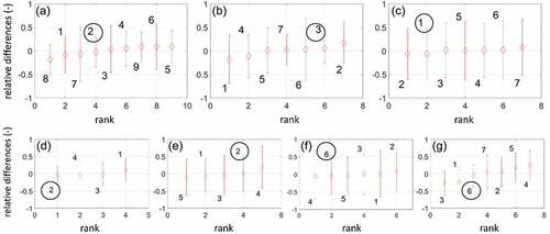
Figure 5. Map of the mean and standard deviation ${\bar{\delta }}_i$ and σ(δ_i), respectively, obtained by the relative differences approach for each rain gauge operative in the study area.

An analysis of frontal systems grouped according to whether ${\bar{R}}_j$ was greater or less than 10 mm was also performed. Table 4 highlights through the σ(δ_i) values the larger dispersion of ${\bar{R}}_j$ for the events with ${\bar{R}}_j$ ≤10 mm.

The existence of a possible link between ${\bar{\delta }}_i$ and the geographical location, elevation above sea level and orographic characteristics was also investigated through multiple regression analysis, but no significant results were obtained.

4.3 Spearman rank correlation coefficient approach

The temporal persistency of the rainfall field was investigated through the Spearman rank correlation coefficient, r_S, using the frontal rainfalls observed within a time period of 10 years. This approach checks if the cumulative rainfall spatial distribution is stable in time, i.e. locations with larger and smaller rainfall keep the same behaviour pattern by changing the spatially average rainfall associated with different fronts. Representative results are shown in Fig. 6 for the Alto Tevere watershed considering two groups of events, each with all the storms characterized by an areal-average cumulative rainfall ≤10 mm (Fig. 6(a)) and >10 mm (Fig. 6(b)), in addition to the group with all the events together (Fig. 6(c)). In each group, there are mostly dark cells, adopted to highlight low r_S values. Light cells, which represent r_S values close to 1, are very limited. White cells are substantially placed only along the diagonal line and refer to the trivial result r_Sjl = 1 for j= l. Furthermore, our results indicate that similar deductions can be applied to different groups of events as those consisting of warm fronts, cold fronts and seasonal frontal systems. As a whole, this Spearman approach does not provide conclusive evidence to enable us to optimize the investigated rain gauge network.

Figure 6. Spearman rank correlation coefficient (r_S, see text) for rainfall frontal systems observed during a 10-year period in the Alto Tevere watershed for events with spatially averaged cumulative rainfall: (a) less than 10 mm and (b) greater than 10 mm, and (c) for all the events.

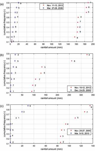
4.4 Frequency distribution

For each watershed, the extreme event characterized by the minimum and maximum value of spatially averaged cumulative rainfall depth (${\bar{R}}_{j\mathrm{m}\mathrm{i}\mathrm{n}}$ and ${\bar{R}}_{j\mathrm{m}\mathrm{a}\mathrm{x}},$ respectively) was considered. The corresponding cumulative frequency distributions were determined by choosing the events with minimum and maximum rainfall in each group (${\bar{R}}_j>10\mathrm{m}\mathrm{m}\mathrm{a}\mathrm{n}\mathrm{d}{\bar{R}}_j$ ≤10 mm). The analysis carried out for each group led to rather similar deductions; therefore, only the results associated with ${\bar{R}}_j$ > 10 mm are explicitly shown in Fig. 7 for three representative watersheds. Comparing minimum and maximum values, it can be seen that there are some unchanged positions (or with a slight difference) in the frequency distribution (see stations 3, 4, 5 and 8 for the Alto Tevere watershed, stations 1, 3, 6 and 7 for the Chiascio, or stations 2 and 6 for the Topino-Marroggia). These outcomes highlight that it is difficult to identify the representative stations directly through the frequency distribution analysis. This limitation appears to be more evident when frontal systems producing ${\bar{R}}_j$ ≤ 10 mm are considered.

Figure 7. Cumulative frequency of significant rainfall frontal systems (with specified front typology and incoming direction deduced from the 700 mb wind) characterized by the minimum and maximum values of the spatially averaged cumulative rainfall depth (>10 mm) observed in the watershed: (a) Alto Tevere (11–13 November 2012: warm, SW; 27–28 March 2008: other, S); (b) Chiascio (10–12 November 2013: other, SW; 24–25 December 2009: warm, SW); and (c) Topino-Marroggia (25–27 November 2005: cold, N; 9–10 March 2010: other, SW). The labels indicate the relative identification numbers of the rain gauges operative in the given watershed (see Table 3).

5 Discussion of results and their application to rain gauge network design

The possibility to determine the areal-average cumulative rainfall produced by frontal systems crossing a given watershed through the use of few “representative” stations identified by the temporal stability analysis has been examined. Because the results derived by the Spearman rank correlation coefficient and the frequency distribution techniques have been found to be not particularly conclusive, this issue has been addressed on the basis of the results derived from the relative difference approach. In this context, it is required to determine a ranking of the rain gauges in each watershed with respect to their accuracy in the representation of both the spatially averaged cumulative rainfall through the N events and the values of ${\bar{R}}_j$ for j= 1, 2, …, N. This implies that the more appropriate stations are characterized by lower values of $\left|{\bar{\delta }}_i\right|$ and σ(δ_i). Considering the possibility of having conflicting results for these two quantities, we adopted as an index of accuracy a quantity – previously used by Zhao et al. (2010) and Penna et al. (2013) for studies of soil moisture content – expressed by:

(6) ${\gamma }_i=\sqrt{{{\bar{\delta }}_i}^2+{\sigma }^2\left({\delta }_i\right)}$(6)

with lower values of γ_i indicating more representative stations. Table 5 summarizes, for each watershed, the values of γ_i obtained from the data highlighted in Fig. 4, for all the frontal systems, and in Table 4 for ${\bar{R}}_j$ less or greater than 10 mm.

Table 4. Mean relative difference, ${\bar{\delta }}_i$, for each rain gauge operative in each watershed and the associated standard deviation, σ(δ_i), for events with cumulative areal-average rainfall, ${\bar{R}}_j$, greater and less than 10 mm.

Watershed	Rain gauge station	${\bar{R}}_j$ ≤ 10 mm		${\bar{R}}_j$ > 10 mm
		${\bar{\delta }}_i$	σ(δi)	${\bar{\delta }}_i$	σ(δi)
Alto Tevere	Cerbara	–0.164	0.463	–0.042	0.332
	Città di Castello	–0.102	0.390	0.013	0.261
	La Cima	0.005	0.582	0.050	0.452
	Petrelle	–0.016	0.443	0.090	0.314
	Pierantonio	0.051	0.393	0.117	0.305
	Ponte Felcino	0.265	0.629	–0.005	0.326
	Ponte Nuovo di Torgiano	0.138	0.815	–0.175	0.356
	San Benedetto Vecchio	–0.198	0.384	–0.169	0.283
	Umbertide	0.021	0.328	0.121	0.303
Chiascio	Bastia Umbra	–0.036	0.731	–0.082	0.584
	Carestello	0.150	0.548	0.077	0.575
	Casa Castalda	0.036	0.347	0.006	0.564
	Gualdo Tadino	–0.209	0.402	–0.069	0.595
	Gubbio	–0.027	0.681	0.051	0.573
	Monte Cucco	0.009	0.886	0.065	0.625
	Pianello	0.077	0.344	–0.048	0.529
Topino-	Azzano	–0.095	0.554	–0.040	0.529
Marroggia	Bevagna	0.011	0.572	–0.119	0.510
	Cannara	0.024	0.642	0.000	0.541
	Foligno	–0.015	0.569	0.029	0.561
	Nocera Umbra	0.046	0.673	–0.014	0.594
	San Silvestro	–0.010	0.692	0.049	0.544
	Spoleto	0.040	0.670	0.094	0.563
Paglia-Chiani	Orvieto	0.096	0.419	0.109	0.252
	Orvieto Scalo	–0.073	0.346	–0.021	0.231
	Ponte Santa Maria	0.005	0.420	–0.040	0.249
	Ponticelli	–0.028	0.436	–0.049	0.297
Nestore	Compignano	–0.150	0.513	–0.064	0.242
	Perugia Santa Giuliana	0.057	0.581	0.020	0.227
	Perugia Sede	0.023	0.626	–0.063	0.226
	Ripalvella	0.248	0.722	0.242	0.411
	San Biagio della Valle	–0.178	0.572	–0.136	0.160
Medio Tevere	Bastardo	0.046	0.752	0.008	0.627
	Casigliano	0.015	0.550	0.143	0.568
	Collepepe	0.019	0.610	0.001	0.542
	Lago di Corbara	0.039	0.842	–0.091	0.519
	Massa Martana	–0.017	0.560	–0.049	0.526
	Todi	–0.101	0.557	–0.012	0.501
Nera	Forsivo	–0.247	0.430	–0.216	0.287
	Narni Scalo	0.066	0.517	0.070	0.367
	Norcia	–0.269	0.416	–0.247	0.333
	Piediluco	0.289	0.576	0.239	0.323
	San Gemini	0.243	0.530	0.130	0.344
	Terni	–0.091	0.369	–0.029	0.270
	Vallo di Nera	0.010	0.549	0.053	0.321

Table 5. Index of accuracy, γ_i, expressed (see Equation (6)(6) ${\gamma }_i=\sqrt{{{\bar{\delta }}_i}^2+{\sigma }^2\left({\delta }_i\right)}$(6) ) through the mean relative difference and associated standard deviation, for each rain gauge operative in each watershed. All: all frontal systems considered (see Fig. 4).

		γi
Watershed	Rain gauge station	All	R≤ 10 mm	R> 10 mm
Alto Tevere	Cerbara	0.395	0.334	0.491
	Città di Castello	0.317	0.261	0.404
	La Cima	0.501	0.455	0.582
	Petrelle	0.371	0.327	0.444
	Pierantonio	0.351	0.327	0.397
	Ponte Felcino	0.479	0.326	0.683
	Ponte Nuovo di Torgiano	0.581	0.397	0.827
	San Benedetto Vecchio	0.368	0.329	0.432
	Umbertide	0.326	0.326	0.329
Chiascio	Bastia Umbra	0.541	0.589	0.732
	Carestello	0.476	0.580	0.568
	Casa Castalda	0.305	0.564	0.349
	Gualdo Tadino	0.463	0.599	0.454
	Gubbio	0.479	0.575	0.682
	Monte Cucco	0.665	0.628	0.886
	Pianello	0.317	0.531	0.352
Topino-	Azzano	0.542	0.531	0.562
Marroggia	Bevagna	0.542	0.523	0.573
	Cannara	0.582	0.541	0.643
	Foligno	0.564	0.562	0.569
	Nocera Umbra	0.625	0.594	0.675
	San Silvestro	0.606	0.546	0.692
	Spoleto	0.611	0.571	0.672
Paglia-Chiani	Orvieto	0.345	0.274	0.430
	Orvieto Scalo	0.287	0.232	0.354
	Ponte Santa Maria	0.330	0.252	0.420
	Ponticelli	0.361	0.301	0.436
Nestore	Compignano	0.510	0.251	0.534
	Perugia Santa Giuliana	0.509	0.228	0.584
	Perugia Sede	0.569	0.234	0.626
	Ripalvella	0.638	0.477	0.763
	San Biagio della Valle	0.528	0.210	0.599
Medio Tevere	Bastardo	0.671	0.627	0.753
	Casigliano	0.573	0.586	0.551
	Collepepe	0.565	0.542	0.611
	Lago di Corbara	0.649	0.527	0.842
	Massa Martana	0.538	0.528	0.560
	Todi	0.523	0.502	0.566
Nera	Forsivo	0.416	0.360	0.496
	Narni Scalo	0.434	0.374	0.521
	Norcia	0.447	0.414	0.496
	Piediluco	0.500	0.402	0.645
	San Gemini	0.458	0.368	0.583
	Terni	0.317	0.272	0.380
	Vallo di Nera	0.490	0.325	0.549

The accuracy in the representation of the mean annual frontal rainfall by low-density networks for ${\bar{R}}_j$ less and greater than 10 mm was examined by selecting 1, 2 and 3 representative stations, with each combination chosen by the lowest values of γ_i. For the Nera watershed, Fig. 8(a) shows that, for ${\bar{R}}_j$ ≤ 10 mm, the use of one representative station produces a great scattering of the results that reduces in the cases of two and mostly three representative stations. A similar trend, but with a fairly limited scattering can be seen in Fig. 8(b) for the same watershed, but for ${\bar{R}}_j$ > 10 mm. The same investigation was performed for all the selected watersheds. Hence, an average analysis of our results for each watershed is performed using the coefficient of determination, R², defined as:

(7) $R^2=1-\left\{\frac{{\sum }_{j=1}^M{\left({\bar{R}}_j-{\bar{R}}_{j,\mathrm{e}\mathrm{s}\mathrm{t}}\right)}^2}{\left[{\sum }_{j=1}^M{\left({\bar{R}}_j-\overline{{\stackrel{ˉ}{R}}_j}\right)}^2\right]}\right\}$(7)

Figure 8. Cumulative rainfall depth represented by different combinations of measurements selected on the basis of the lowest values of the accuracy index given in Table 5 vs mean areal cumulative rainfall, for the events with depth (a) less than and (b) greater than 10 mm. Nera watershed.

where ${\bar{R}}_{j,\mathrm{e}\mathrm{s}\mathrm{t}}$ is the value of ${\bar{R}}_j$ approximated by the arithmetic mean of R_ij obtained through the representative stations and $\overline{{\stackrel{ˉ}{R}}_j}$ is the arithmetic mean value of ${\bar{R}}_j$ computed for the M frontal events.

Table 6 provides R² associated with each watershed for ${\bar{R}}_j$ less and greater than 10 mm, as well as for all the events together.

Table 6. Coefficient of determination, R², associated with each watershed for the use of different combinations of representative stations defined through the temporal stability analysis. Combination 1 refers to the station with the lowest value of γ_i (see Table 5); combination 2 refers to the first and second lowest values of γ_i; and combination 3 refers to the first, second and third lowest values of γ_i. Three groups of events put together on the basis of the cumulative areal-average rainfall depth, ${\bar{R}}_j$, are considered.

Watershed	Combination 1	Combination 2	Combination 3
All rainfall events
Alto Tevere	0.947	0.977	0.984
Chiascio	0.917	0.921	0.967
Medio Tevere	0.943	0.958	0.976
Nera	0.812	0.957	0.965
Nestore	0.968	0.990	0.993
Paglia-Chiani	0.947	0.994	0.992
Topino-Marroggia	0.911	0.963	0.955
Average	0.921	0.966	0.976
${\bar{R}}_j$ ≤ 10 mm
Alto Tevere	0.527	0.761	0.837
Chiascio	0.594	0.662	0.723
Medio Tevere	0.559	0.704	0.838
Nera	0.440	0.637	0.745
Nestore	0.418	0.785	0.836
Paglia-Chiani	0.584	0.953	0.918
Topino-Marroggia	0.523	0.790	0.805
Average	0.521	0.756	0.815
${\bar{R}}_j$ > 10 mm
Alto Tevere	0.941	0.974	0.982
Chiascio	0.902	0.906	0.962
Medio Tevere	0.930	0.948	0.971
Nera	0.762	0.952	0.957
Nestore	0.967	0.989	0.992
Paglia-Chiani	0.943	0.994	0.991
Topino-Marroggia	0.887	0.952	0.944
Average	0.905	0.959	0.971

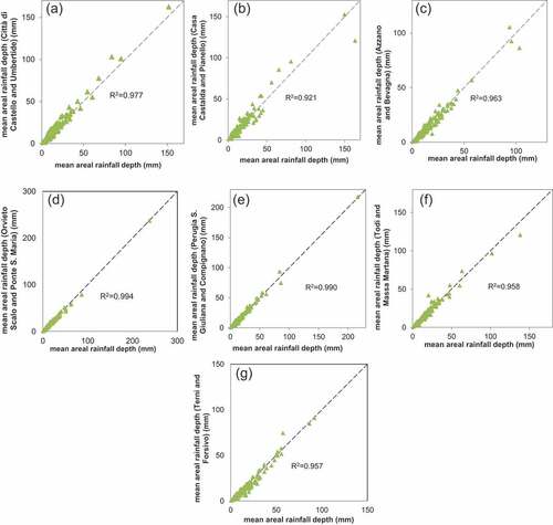
As can be seen in Table 6, for the events with ${\bar{R}}_j$ ≤ 10 mm, there is generally a considerable increase in R² with increasing number of representative rain gauges, from 1 to 2 and 3, with average values of 0.521, 0.756 and 0.815, respectively. The same trend is highlighted for ${\bar{R}}_j$ > 10 mm, but with much higher R² values, even in the case of a sole representative station characterized by only three watersheds, with R² less than the average value of 0.905. Furthermore, considering all the frontal systems together, Table 6 shows satisfactory values, even in the case of a sole representative station, with an average R² of 0.921 and a minimum of 0.812 for the Nera watershed, and improved R² values in the other two combinations. Really, with two and three representative stations, the values of R² are almost the same (0.966 and 0.976, respectively). On this basis, considering the need to minimize the rain gauge network density keeping significant values of R², the best configuration should be chosen between those with a sole representative rain gauge or two representative stations in each watershed. Figures 9 and 10 show the approximation of ${\bar{R}}_j$ (j= 1, 2, …, M) in each watershed by adopting the solutions with one and two representative rain gauges, respectively. As can be seen in Figs. 9 and 10, the transition from 1 to 2 representative stations produces an appreciable improvement of the approximated estimate of ${\bar{R}}_j$ in all the watersheds that is not linked with the watershed area. This is supported by the reduced scattering of results in each watershed that is more pronounced, at least in relative terms, for light and moderate frontal systems. In any case, for significant frontal systems, the relative error in the estimate of ${\bar{R}}_j$ is in magnitude within 10%. Therefore, the best rain gauge network, independently of the watershed area, is that associated with two representative stations with location identified by the relative difference approach for the temporal stability analysis.

Figure 9. Mean areal cumulative rainfall depth approximated in each watershed by the more representative station vs its value derived from all the operative stations, for all observed frontal systems: (a) Alto-Tevere, (b) Chiascio, (c) Topino-Marroggia, (d) Paglia-Chiani, (e) Nestore, (f) Medio Tevere, and (g) Nera. The determination coefficients, R², are also reported.

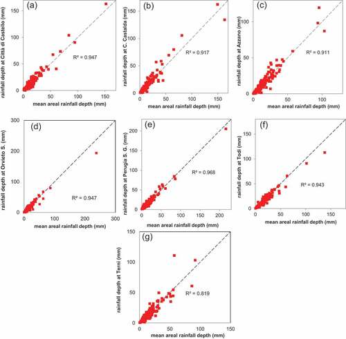
Figure 10. Mean areal cumulative rainfall depth approximated in each watershed by the two more representative stations vs its value derived from all the operative stations, for all observed frontal systems: (a) Alto-Tevere, (b) Chiascio, (c) Topino-Marroggia, (d) Paglia-Chiani, (e) Nestore, (f) Medio Tevere, and (g) Nera. The determination coefficients, R², are also reported.

The considerable accuracy in the estimate of ${\bar{R}}_j$, using the above procedure for selecting the best two rain gauges characterized by temporal stability, suggests that in each watershed these stations have on average a ranking, with respect to the values of R_ij (i= 1, 2, …, N), which remains invariant throughout the significant frontal systems. In addition, in each watershed, there are a few other stations, with values of γ_i rather close to the two best ones (Table 5), to which the same deduction can be approximately applied. However, other stations with significantly larger values of γ_i do not show this property. Figure 2 supports this reasoning for a sample watershed.

The localization of the selected stations (see also Fig. 11) can be linked with results obtained previously by Corradini (1985) and Corradini and Melone (1989). Specifically, they detected orographic enhancement of rain in the prefrontal and postfrontal stages of cold fronts and ahead of surface warm fronts, while weakening or dissipation of pre-existing SMSAs due to orography was observed for a significant number of cold fronts. The last results were obtained using a high-density rain gauge network specifically set-up to investigate the orographic effects on rainfall spatial distribution at the meso-local scale. Significant enhancement of rain in warm fronts was generated, through a seeder-feeder mechanism (Cotton et al. 2011), downwind of regions with forced uplift of air mass over an envelope type orography with smoothing of isolated peaks and narrow valleys (Corradini 1985). However, dissipation or weakening of pre-existing SMSAs in cold fronts was linked to a deflection of air mass by a steep and continuous orographic barrier that inhibited the forced uplift when low wind velocities were involved.

Figure 11. Map of the study area with the more representative rain gauge stations. Identification numbers are listed in Table 1.

On the above basis, none of the representative rain gauges selected by the temporal stability approach was operative in locations where these types of changes in rainfall could be significant. Their outcomes were suggested by the orientation of the hilly and mountainous terrain with respect to prevailing surface wind direction which was in the range between south and west-southwest, while the incoming direction of the frontal systems deduced from the 700 mb wind (Table 2) was mainly between southwest and northwest. On this basis, the areas prone to the production of the above orographic effects are those oriented between west–east and northwest–southwest. The outcomes of our study on the localization of the representative stations, identified by the temporal stability analysis, interpreted on the basis of the interaction between dynamics of frontal systems and orography, can represent a useful insight even for rain gauge network design in ungauged watersheds.

Incidentally, the possibility of using the representative rain gauges selected by the temporal stability analysis applied to the cumulative rainfall depth for estimating, for each front, the time evolution of ${\bar{R}}_j$ was also examined. Figure 12 shows the results obtained for two sample events that occurred in two watersheds and produced by two different front types coming from the southwest. Figure 12(a) refers to a cold front over the Alto Tevere watershed, with ${\bar{R}}_j$ derived from all the operative devices of 21.6 mm and ${\bar{R}}_{j,\mathrm{e}\mathrm{s}\mathrm{t}}$ of 21.8 mm, while Fig. 12(b) is relative to a warm front over the Chiascio watershed, with ${\bar{R}}_j$ of 30.5 mm and ${\bar{R}}_{j,\mathrm{e}\mathrm{s}\mathrm{t}}$ of 31.9 mm. In addition to the cumulative rainfall depths, the shapes of the two hyetographs deduced by all the operative rain gauges are also fairly well reproduced by the two representative stations; however, in a few time intervals, the errors in rainfall depth are significant enough. In any case, when rainfall is an input in lumped rainfall–runoff models, the adoption of the hyetograph obtained by two representative stations appears to be sufficiently appropriate, even though a reformulation of the temporal stability analysis based on the use of hourly rainfall within each frontal system could improve the results.

Figure 12. Comparison of hyetographs deduced by all the gauges operative in a watershed and derived from the two best stations defined through the temporal stability analysis: (a) Alto Tevere, and (b) Chiascio.

6 Conclusions

In spite of a variety of studies having been carried out for optimizing rain gauge networks, the methods available for specific hydrological applications requiring rainfall as the input still need to be substantially improved. These methods are commonly based on statistical elements, while the mechanisms producing rainfall spatial variability have a minor role (Mishra and Singh 2017). Investigations of the problem restricted to specific types of meteorological systems, such as, for example, large frontal disturbances or convective systems, can be of utmost importance. The proposed approach provides further insights for rain gauge networks finalized to the determination of rainfall produced by frontal systems, which give an important contribution to precipitation at mid-latitudes.

Having been developed in the light of an optimal network design for representing the cumulative areal-average rainfall depth for any typology of frontal system, our study indicates that:

1. The proposed methodology, based on the use of temporal stability analysis performed with the relative differences approach, provides proper solutions of the problem in each watershed through a combination of the observations carried out in stations with better ranking in approximating singly ${\bar{R}}_j$ deduced from all the operative stations. In each selected watershed (area up to 1536 km²) a combination of two rain gauges was found to give a fairly good representation of ${\bar{R}}_j$, particularly for significant frontal systems, with the magnitude of the relative error generally less than 10%.

2. The appropriate locations of the representative stations in an ungauged watershed can be deduced by considering the role of orography with respect to the prevailing incoming directions of the frontal systems, especially for rainfall events with a mean areal rainfall depth larger than 10 mm.

3. The methodology set-up for the cumulative rainfall depths provides a fairly good representation of the main features of the areal-average hyetographs of each watershed.

A reformulation of the temporal stability analysis considering hourly rainfall in each frontal system together with an in-depth analysis of the critical issues related to events with ${\bar{R}}_j$ ≤ 10 mm would be required to obtain an optimal network design appropriate to further improve the results of point (3) and to have a sufficiently detailed knowledge of the rainfall spatial distribution for its use as input to distributed rainfall–runoff models. In any case, a rain gauge network optimized to determine the areal-average cumulative rainfall is important for the application of lumped rainfall–runoff models, as well as for its use in the hydrological practice.

Acknowledgements

The authors are thankful to the Umbria Region and its Functional Centre for providing the rainfall data and N. Feliciani and M. Stelluti for their technical assistance.

Disclosure statement

No potential conflict of interest was reported by the authors.

References

- Adhikary, S.K., Muttil, N., and Yilmaz, A.G., 2017. Improving streamflow forecast using optimal raingauge network-based input to artificial neural network models. Hydrology Research, IWA, 49, 1559–1577.
- Adhikary, S.K., Yilmaz, A.G., and Muttil, N., 2015. Optimal design of raingauge network in the Middle Yarra River catchment, (Australia). Hydrological Processes, 29, 2582–2599. doi:10.1002/hyp.10389
- Bardossy, A. and Das, T., 2006. Influence of rainfall observation network on model calibration and application. Hydrology and Earth System Sciences Discussion, 3, 3691–3726. doi:10.5194/hessd-3-3691-2006
- Beven, K., 2001. How far can we go in distributed hydrological modelling? Hydrology and Earth System Sciences, 5 (1), 1–12. doi:10.5194/hess-5-1-2001
- Brocca, L., et al., 2009. Soil moisture temporal stability over experimental areas of Central Italy. Geoderma, 148, 364–374. doi:10.1016/j.geoderma.2008.11.004
- Brocca, L., et al., 2010. Spatial-temporal variability of soil moisture and its estimation across scales. Water Resources Research, 46, W02516. doi:10.1029/2009WR008016
- Brocca, L., et al., 2012. Catchment scale soil moisture spatial-temporal variability. Journal of Hydrology, 422–423, 63–75. doi:10.1016/j.jhydrol.2011.12.039
- Browning, K.A., 1985. Conceptual models of precipitation systems. The Meteorological Magazine, 114, 293–319.
- Browning, K.A., Hill, F.F., and Pardoe, C.W., 1974. Structure and mechanism of precipitation and the effect of orography in a wintertime warm sector. Quarterly Journal of the Royal Meteorological Society, 100, 309–330. doi:10.1002/(ISSN)1477-870X
- Browning, K.A., Pardoe, C.W., and Hill, F.F., 1975. The nature of orographic rain at wintertime cold fronts. Quarterly Journal of the Royal Meteorological Society, 101, 333–352. doi:10.1002/(ISSN)1477-870X
- Chacon-Hurtado, J.C., Alfonso, L., and Solomatine, D.P., 2017. Rainfall and streamflow sensor network design: a review of applications, classification, and a proposed framework. Hydrology and Earth System Science, 21, 3071–3091. doi:10.5194/hess-21-3071-2017
- Corradini, C., 1985. Analysis of the effects of orography on surface rainfall by a parameterized numerical model. Journal of Hydrology, 77, 19–30. doi:10.1016/0022-1694(85)90195-7
- Corradini, C., 2014. Soil moisture in the development of hydrological processes and its determination at different spatial scales. Journal of Hydrology, 516, 1–5. doi:10.1016/j.jhydrol.2014.02.051
- Corradini, C. and Melone, F., 1989. Spatial structure of rainfall in mid-latitude cold front systems. Journal of Hydrology, 105, 297–316. doi:10.1016/0022-1694(89)90110-8
- Cotton, W.R., Bryan, G.H., and van den Heever, S.C., 2011. The influence of mountains on airflow, clouds, and precipitation. In: R. Dmowska, D. Hartmenn, and H.T. Rossby, eds. Storm and cloud dynamics, vol. 99, international geophysics series. USA: Academic Press, 673–750.
- Dong, X., Dohmen-Janssen, M., and Booij, M.J., 2005. Appropriate spatial sampling of rainfall for flow simulation. Hydrological Sciences Journal, 50 (2), 279–298. doi:10.1623/hysj.50.2.279.61801
- Georgakakos, K.P., Bae, D.H., and Cayan, D.R., 1995. Hydroclimatology of continental watersheds: 1. Temporal analyses. Water Resources Research, 31 (3), 655–675. doi:10.1029/94WR02375
- Gong, Y., et al., 2018. Influence of rainfall, model parameters and routing methods on stormwater modelling. Water Resources Management, 32 (2), 735–750. doi:10.1007/s11269-017-1836-x
- Grayson, R.B. and Blöschl, G., ed., 2000. Spatial patterns in catchment hydrology: observations and modelling. Cambridge: Cambridge University Press.
- Grayson, R.B. and Western, A.W., 1998. Towards areal estimation of soil water content from point measurements: time and space stability of mean response. Journal of Hydrology, 207, 68–82. doi:10.1016/S0022-1694(98)00096-1
- Khaliq, M.N., et al., 2009. Identification of hydrological trends in the presence of serial and cross correlation: A review of selected methods and their application to annual flow regimes of Canadian rivers. Journal of Hydrology, 368, 117–130. doi:10.1016/j.jhydrol.2009.01.035
- Krstanovic, P.F. and Singh, V.P., 1992a. Evaluation of rainfall networks using entropy: 1. Theoretical development. Water Resources Management, 6, 279–293. doi:10.1007/BF00872281
- Krstanovic, P.F. and Singh, V.P., 1992b. Evaluation of rainfall networks using entropy: 2. Application. Water Resources Management, 6, 295–314. doi:10.1007/BF00872282
- Kundzewicz, Z.W., 1997. Water resources for sustainable development. Hydrological Sciences Journal, 42 (4), 467–480. doi:10.1080/02626669709492047
- Markus, M., Knapp, H.V., and Tasker, G.D., 2003. Entropy and generalized least square methods in assessment of the regional value of streamgages. Journal of Hydrology, 283, 107–121. doi:10.1016/S0022-1694(03)00244-0
- Melone, F., Corradini, C., and Singh, V.P., 1998. Simulation of the direct runoff hydrograph at basin outlet. Hydrological Processes, 12 (5), 769–779. doi:10.1002/(ISSN)1099-1085
- Mishra, A.K. and Singh, V.P., 2017. Design of hydrologic networks. In: V.P. Singh, eds. Handbook of applied hydrology. 2nd ed. New York: McGraw-Hill, 10.1–10.5.
- Molina, A.J., et al., 2014. Spatio-temporal variability of soil water content on the local scale in a Mediterranean mountain area (Vallcebre, North Eastern Spain). How different spatio-temporal scales reflect mean soil water content. Journal of Hydrology, 516, 182–192. doi:10.1016/j.jhydrol.2014.01.040
- Munoz, B., Lesser, V.M., and Ramsey, F.L., 2008. Design-based empirical orthogonal function model for environmental monitoring data analysis. Environmetrics, 19 (8), 805–817. doi:10.1002/env.v19:8
- Penna, D., et al., 2013. Soil moisture temporal stability at different depths on two alpine hillslopes during wet and dry periods. Journal of Hydrology, 477, 55–71. doi:10.1016/j.jhydrol.2012.10.052
- Rivera, D., et al., 2012. A methodology to identify representative configurations of sensors for monitoring soil moisture. Environmental Monitoring and Assessment, 184 (11), 6563–6574. doi:10.1007/s10661-011-2441-8
- Rodriguez-Iturbe, I. and Mejia, J.M., 1974. The design of rainfall network in time and space. Water Resources Management, 10 (4), 713–728. doi:10.1029/WR010i004p00713
- Sneyers, R., Vandiepenbeeck, M., and Vanlierde, R., 1989. Principal component analysis of Belgian rainfall. Theoretical and Applied Climatology, 39, 199–204. doi:10.1007/BF00867948
- Stokstad, E., 1999. Scarcity of rain, stream gages threaten forecasts. Science, 285 (5431), 1199–1200. doi:10.1126/science.285.5431.1199
- Vachaud, G.A., et al., 1985. Temporal stability of spatially measured soil water probability density function. Soil Science Society of America Journal, 49, 822–828. doi:10.2136/sssaj1985.03615995004900040006x
- Wang, W., et al., 2018. Optimization of rainfall networks using information entropy and temporal variability analysis. Journal of Hydrology, 559, 136–155. doi:10.1016/j.jhydrol.2018.02.010
- Zhao, S., et al., 2010. Controls of surface soil moisture spatial patterns and their temporal stability in a semi-arid steppe. Hydrological Processes, 24, 2507–2519. doi:10.1002/hyp.7665