On the use of mean monthly runoff to predict the flow–duration curve in ungauged catchments

ABSTRACT

We examine the applicability of predicting the daily flow–duration curve (FDC) using mean monthly runoff represented in its stochastic form (MM_FDC) to aid in predictions in ungauged basins, using long-term hydroclimatic data at 73 catchments of humid climate, in the eastern USA. The analysis uses soil hydrological properties, soil moisture storage capacity and the predominant runoff generation mechanism. The results show that MM_FDC did not distinguish the shapes of the upper and lower thirds of the FDC. The upper third is where the precipitation pattern and the antecedent moisture conditions are dominant, while the lower third is where drought-induced low flows and the evapotranspiration effect are prevalent. It is possible to use the MM_FDC to predict the middle third of the FDC (exceedence probabilities between 33% and 66%). The method is constrained by the catchment flow variability (slope of FDC), which changes in accordance with landscape properties and the predominant runoff generation mechanism.

KEYWORDS:

• mean monthly runoff
• flow–duration curve
• flow variability
• landscape characteristics
• runoff generation mechanism

Editor R. Woods ; Associate editor T. Okruszko

1 Introduction

The prediction and characterization of the flow regime are critical for management of water resources and aquatic ecosystems (Poff et al. 1997). They are also relevant for public safety as they help in protecting against floods, and allow the quantification of water supplies during droughts (Muneepeerakul et al. 2010). A central problem of hydrology is understanding the processes that affect streamflow and making predictions in river basins (Botter et al. 2009, Booker and Snelder 2012, Ameli et al. 2015), a process made particularly difficult in basins where measured hydroclimatic data are not available.

The flow–duration curve (FDC) characterizes the flow regime within a stochastic framework. The FDC is a graphical representation of the frequency, or the fraction of time during which a specified magnitude of runoff is equalled or exceeded (Vogel and Fennessey 1994, Castellarin et al. 2013). The FDC is relevant for many hydrological applications, including the management of aquatic systems, flooding and drought, in addition to lake sedimentation studies, water quality management and water resources allocation (Vogel and Fennessey 1995, Atieh et al. 2017).

The FDC prediction in ungauged catchments traditionally consists of two steps. First, the FDC distribution parameters are determined for gauged catchments using streamflow observations and curve fitting (Booker and Snelder 2012). In the second step, a regional regression model is developed by (i) predicting the statistical distribution parameters for ungauged catchments from the physiographic and climatic characteristics of the catchments (LeBoutillier and Waylen 1993, Smakhtin et al. 1997, Singh et al. 2001, Holmes et al. 2002, Sauquet and Catalogne 2011, Pugliese et al. 2016), (ii) deriving a regional non-dimensional distribution using daily flows of gauged catchments of a homogeneous region, which is subsequently multiplied by the index flow at the ungauged catchments, determined by mapping and interpolations (Vandewiele and Elias 1995, Razavi and Coulibaly 2012, Blöschl et al. 2013), or (iii) through correlation with the basin characteristics (Claps and Fiorentino 1997, Castellarin et al. 2004, Razavi and Coulibaly 2012, Requena et al. 2018). The FDC at an ungauged site can also be obtained from FDC at a gauged site by using a dissimilarity method (Ganora et al. 2009). The method of Ganora et al. (2009) is based on the value of a dissimilarity index between pairs of catchments. The dissimilarity index is calculated using values of the basin descriptors (e.g. area, mean elevation, mean slope and drainage path length). The difference in dissimilarity indices for each pair of catchments helps to cluster “similar” catchments; the smaller the value of the dissimilarity index the more “similar” are the catchments (Ganora et al. 2009). Recently, another technique that employed the kriging interpolation (Castellarin 2014, Castellarin et al. 2018) has shown to be particularly accurate and easily applicable over large geographical areas.

Despite their utility, process-based studies that predict the FDC for ungauged catchments are rare (e.g. Botter et al. 2007a, 2007b, 2009, Muneepeerakul et al. 2010, Yokoo and Sivapalan 2011). Process-based stochastic models that predict the FDC have been tested; however, they have not been validated in actual catchments across a range of topographic and hydroclimatic settings (Botter et al. 2007a, 2007b, 2009, Muneepeerakul et al. 2010, Yokoo and Sivapalan 2011). Botter et al. (2007a) developed a stochastic model of the subsurface flow to predict the overall streamflow response. The stochastic dynamic model was used to analytically derive FDCs in a few catchments in both the USA and Europe (Botter et al. 2007b, 2010, Ceola et al. 2010). The stochastic model used physical parameters that can be easily determined for ungauged catchments, including soil, vegetation and geomorphic attributes (mean residence time of subsurface flow and the size of the basin). The model could only be applied seasonally with constant parameter values for each season. Muneepeerakul et al. (2010) complemented the work of Botter et al. (2007a, 2007b) adding the surface flow component (fast flow) using a stochastic model of rainfall–streamflow generation. Testing the model in a few catchments showed that complex streamflow processes can be captured by separately simulating the surface and subsurface flows. However, this stochastic modelling framework has not been validated in watersheds of different sizes, geological settings and climate.

The theoretical study by Yokoo and Sivapalan (2011) tested the effect of several combinations of climate and landscape properties, using a hypothetical catchment, on the shape of the FDC in relation to the mean monthly runoff represented in its stochastic form (MM_FDC). The study used three years of synthetic rainfall time series to run a water balance model that makes use of climate, geographical parameters (e.g. depth of soil layer, average thickness of saturated zone) and soil parameters (e.g. hydraulic conductivity, porosity). The investigation invoked the simulated flow components of the FDC (surface flow FDC and subsurface flow FDC). The study tested the effect of climate (humid vs dry), soil type (silt vs sand) and soil depth (shallow vs deep) in conditions of different climate seasonality (precipitation in phase/out of phase with potential evapotranspiration). Yokoo and Sivapalan (2011) conjectured that the upper third of the FDC is determined by a non-linear transformation of the precipitation. In catchments with perennial flow and humid climate, Yokoo and Sivapalan (2011) hypothesized that the middle and the lower third are represented by the mean monthly runoff data that might need corrections to account for the effect of evapotranspiration (ET) on low flows in order to predict the FDC lower third. In catchments with ephemeral flows, the conjectures about the use of the mean monthly runoff data are not applicable. The conceptual model of Yokoo and Sivapalan (2011) is intended to facilitate predictions for ungauged catchments – at least in a humid climate – through extrapolation from gauged catchments of daily precipitation, monthly flow, climate dryness and storage capacity (needed for the effect of ET). Precipitation data are often available at ungauged catchments (e.g. weighted average from raingauges, global or regional climate reanalysis (Feser et al. 2011)) and by extrapolation from gauged catchments via a hydro-climatic classification system (Coopesmith et al. 2014).

The mean monthly runoff is relatively easy to obtain for ungauged catchments from predictions of global hydrological models (GHMs) (e.g. Xie and Arkin 1996, Nijssen et al. 2001). We acknowledge that more detailed information than mean monthly runoff can be obtained from GHMs, such as one-day time resolution data (Sood and Smakhtin 2015). However, the use of this information requires further investigation. The meteorological data used to run GHMs can be obtained from global climate models (GCMs), or from spatial interpolation and observation networks (e.g. the DAYMET database). The former is considered unreliable at time scales shorter than 1 month and does not provide reliable estimates of rainfall variance, making it difficult to develop appropriate downscaling methodologies (Prudhomme et al. 2002), while the latter have climate time series that extend only into the 1980s or so (Sood and Smakhtin 2015). Therefore, global models would be more efficient at a monthly than a daily time step. Further investigation is needed to validate the use of GHMs at the daily time step.

The use of mean monthly data would also be valuable when flow data at the daily time scale are not available in the neighbouring “similar” gauged catchments. The findings and hypotheses of Yokoo and Sivapalan (2011) were based on a conceptual investigation using one theoretical catchment and hypothetical combinations of climate and landscape characteristics. Therefore, there is a need to develop and test hypotheses on actual catchments that will advance the process understanding and prediction of FDCs for ungauged catchments using monthly flow data.

Our objective was to extend the work of Yokoo and Sivapalan (2011) to real catchments with varying characteristics and flow regimes. We investigated the use of mean monthly flow when represented in its stochastic form (MM_FDC) to make estimates of the FDC across many catchments at the regional scale. In this study, our line of reasoning is: (a) to do a meta-analysis using different sites (73 catchments) of heterogeneous hydroclimate characteristics and learn from the data to find out patterns of change in FDC and MM_FDC; and (b) to understand the patterns, providing technical and physical explanations and set hypotheses that will be subject to testing in future studies. Testing the hypotheses will help in designing the prediction model of the FDC using the MM_FDC. This model is more widely applicable because it is developed from a large spectrum of heterogeneity in characteristics and process mechanisms offered by the multiple sites (Sivapalan et al. 2003).

By definition, a meta-analysis is the approach of combining qualitative and quantitative data from several sites/studies to develop conclusions that have greater statistical power (Barthold and Woods 2015, Evaristo and McDonnell 2017). The meta-analysis provides an objective measure and is a useful platform for generating large-scale conclusions (Evaristo and McDonnell 2017). Meta-analysis studies are of great value in hydrology and have recently been used to identify key characteristics of the hydrological responses of Mediterranean catchments at different time scales (Merheb et al. 2016). The meta-analysis has applications not only in hydrology but also in other disciplines, such as epidemiology (Greenland et al. 2008).

The line of reasoning we propose here is a top-down approach (Sivapalan et al. 2003), which provides a systematic framework to learn from the data, including setting the hypotheses and testing them in following stages. This approach is in contrast to a bottom-up approach in catchment hydrology (Ye et al. 2012), which predicts the catchment response from smaller-scale understanding of the processes (starting with setting the hypotheses, collecting and analysing the data and developing the conceptual predictive model). From this perspective, the predictive models require up-scaling to conduct analyses at larger scales (catchment or regional) (Klemeš 1983, Sivapalan et al. 2003). However, extrapolation and prediction of catchment responses across different places and a range of scales is a challenging problem in hydrology (Beven 1989, 2000, Grayson et al. 2002).

The results of our regional study, namely, the observed patterns, the physical explanations and the hypotheses, will advance our understanding and contribute to the wider objective of developing an FDC predictive model – on a physical basis – to enable prediction in ungauged catchments. Barthold and Woods (2015), using a meta-analysis of several sites and studies, concluded that progress in hydrology requires knowledge to be synthesized in order to develop prediction models that are applicable to a wide range of environmental conditions and that facilitate prediction in ungauged catchments.

We conduct our analysis in the eastern USA using outcomes of the environmental controls of the FDC in Chouaib et al. (2018) (e.g. soil moisture storage capacity, topography and predominant runoff generation mechanisms). The outcomes described in Chouaib et al. (2018) support the results of the meta-analysis. The results of the current study will further our understanding about the conditions that limit the use of the MM_FDC in prediction of the FDC. The meta-analysis takes advantage of the diversity in hydroclimate conditions and properties of the flow variability (steep vs flatter slopes of the FDC) across the study catchments.

In this study, we use observed mean monthly flows to construct the MM_FDCs and daily flows to construct the FDCs. To test/verify the use of predicted mean monthly flows from a regionalization approach compared to those from GHMs was beyond the scope of our study. It is assumed that an exact prediction of the mean monthly flow will be available at the ungauged catchment and we admit the attributed uncertainty resulting from the use of a GHM or a regionalization approach. The uncertainty of the mean monthly predictions using GHMs is amenable to improvements (Sood and Smakhtin 2015).

2 Dataset and study area

In this study, we use the Model Parameter Estimation Experiment (MOPEX) catchments of Chouaib et al. (2018) that are located in the eastern USA. The MOPEX dataset provides the data in each catchment (Duan et al. 2006). In MOPEX, the hydro-meteorological records (i.e. air temperature, precipitation, potential evapotranspiration and flow) have a daily time step and 50 years length on average (1948–2000). More details about the MOPEX dataset are provided in Chouaib et al. (2018, Section 2). The MOPEX dataset provides flow and meteorological data in addition to physiographic characteristics for many catchments in the USA and other countries (Duan et al. 2006). Several hydrologists and modellers have collaborated to develop the MOPEX dataset and share expertise in modelling and parameter estimation. These collaborations put the MOPEX dataset in the forefront for use in studies of prediction in ungauged catchments (Hrachowitz et al. 2013). In the eastern USA, precipitation has a limited seasonal fluctuation (Sawicz et al. 2011, Coopersmith et al. 2012, Chouaib et al. 2018). The catchments are medium to large (67–8052 km²), as shown in Table 1. These catchments are mainly forested, with some agricultural lands and a limited influence of urban areas (Table 1). The Appalachian Mountains, which characterize the topography of the study area (see the digital elevation model, DEM in Fig. 1) have a northeast to southwest orientation. In terms of the soil characteristics, the proportion of soil with medium infiltration rate (HGB soils; Wood and Blackburn 1984) decreases from south to north, while the proportion of soil with slow infiltration rate (HGC soils; Wood and Blackburn 1984) declines from north to south (Fig. 1).

Table 1. Statistics of the catchments used in this study. MAP: mean annual precipitation.

Catchment descriptor	Maximum	Minimum	Median
Slope (%)	34	0.6	12.7
Mean elevation (m a.s.l.)	1212	16.2	442.6
Land cover – Crops (%)	59	0	15.8
Land cover – Forest (%)	98	28.64	65.68
Land cover – Urban (%)	18.67	0	6.3
Catchment size (km^2)	8052	67	1170.70
MAP (mm)	2072	982	1199

Figure 1. Map of the study site showing the spatial distribution of the soil hydrologic groups: (a) HGB and (b) HGC.

3 Methods

3.1 Sacramento model (SAC-SMA) calibration

We use the Sacramento soil moisture accounting (SAC-SMA) model to assess the surface and subsurface flow FDCs that will support our investigation of the MM_FDC in relation to the FDC. Details of the hydrological model can be found in Chouaib et al. (2018). The SAC-SMA model is calibrated in each of the study catchments that have limited snow effect. We designate the study catchment as having limited snow effect because the perennial snow cover is absent for most catchments and does not exceed 3% of the surface area in individual catchments (Berghuijs et al. 2014). We used a sample of 100 catchments of limited snow effect for calibration, and those with a Nash-Sutcliffe coefficient (NS; Nash and Sutcliffe 1970) of less than 0.50 were disregarded; we retained 73 catchments after the calibration. Model performance, in particular for surface and subsurface flow predictions that are used in the analysis, was not used to check the results of this study, because the efficiency of the SAC-SMA calibration was satisfactory (Chouaib et al. 2018). As seen in Fig. 2, we found that 90% of the catchments have NS > 0.6.

Figure 2. Performance of the study catchments after calibration using the NS coefficient.

3.2 Analysis of the MM_FDC in relation to the FDC

The MM_FDC is constructed from the average of all flows that fall in each month over the entire period of flow records (50 years on average) following the theoretical study by Yokoo and Sivapalan (2011). The MM_FDC in each study catchment has 12 readings (one for each month). The FDC is constructed from the daily flows of the entire period of record.

We normalized the empirical FDCs and MM_FDCs by the value of the mean flows, as in Yokoo and Sivapalan (2011) and Yaeger et al. (2012). We calculated the slopes of the normalized FDCs using the 33rd and 66th flow percentiles (Equation 1). This is the most linear portion of the curve at a semi-logarithmic scale (Yadav et al. 2007, Zhang et al. 2008). This portion of the curve indicates the value of the flow variability (Sawicz et al. 2011). The slope of the FDC, SFDC, is defined as:

(1) $\mathrm{S}\mathrm{F}\mathrm{D}\mathrm{C}=\frac{ln\left(Q33\mathrm{\%}\right)-\mathrm{l}\mathrm{n}\left(Q66\mathrm{\%}\right)}{\left(0.66-0.33\right)}$(1)

where Q33% is the flow of the 33rd percentile and Q66% is the flow of the 66th percentile. We calculated the slope of the normalized MM_FDC (SMM_FDC) from the value of the highest and lowest flow percentiles, as in Yaeger et al. (2012). We examined the correlation between the slopes of MM_FDC and FDC using a linear regression. We wanted to determine how well correlated the two curves are before developing a detailed analysis of the MM_FDC. The SFDC helped us differentiate between the characteristics of the flow response in the study catchment. In catchments with SFDC below the average (across all catchments), the flow variability is regarded as low, with a flatter shape of the FDC. In catchments with SFDC above the average, the flow variability is higher, with a steeper slope of the FDC.

We compared the spatial pattern of the SMM_FDC and SFDC to determine whether a catchment with a steep SFDC had a steep SMM_FDC. This comparison revealed whether the spatial pattern of the FDC was similar to that of the MM_FDC. We compared each of the FDC portions (the upper, middle and lower thirds of the FDC) to the MM_FDC, as in Yokoo and Sivapalan (2011). However, our comparison differentiated between categories of the flow variability and used real catchments instead of hypothetical catchments. The meta-analysis accounts for the disparities in landscape properties. The real combinations of catchment characteristics reveal the physical conditions where it is (or is not) possible to predict FDC from the MM_FDC. The meta-analysis uses also the flow components of the FDC to explain the processes underlying each of the FDC portions and further explore the physical conditions allowing prediction of the FDC from the MM_FDC.

4 Results

4.1 Variation of the MM_FDC in comparison to the FDC

The regional variation of the SMM_FDC is equivalent to the regional variation of the SFDC (Fig. 3(a) and (b)). The catchments with large SFDC in Fig. 3(a) are mostly those having steeper slope of the MM_FDC in Fig. 3(b). This is corroborated by a statistically significant correlation between the middle thirds of the FDC (SFDC) and the SMM_FDC (p < 0.05) (Fig. 3(c)). However, the SMM_FDC explains 38% of the SFDC variation.

Figure 3. Regional variation of (a) the slope of the FDC (SFDC), (b) the mean monthly FDC (MM_FDC), and (c) the correlation between the SFDC and the slope of the MM_FDC (SMM_FDC).

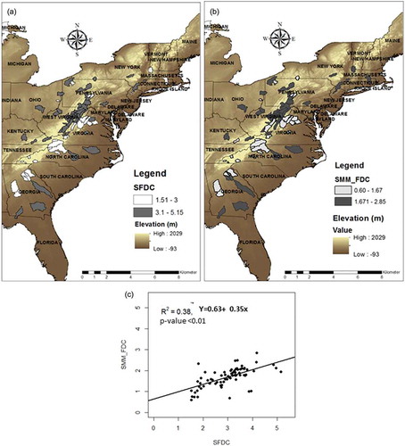
The difference in shape of the FDCs based on their slope is equivalent to the difference in shape of the MM_FDCs. The MM_FDCs of catchments with large SFDC have steeper slopes than those of catchments with small SFDC (Fig. 4(a) and (b)).

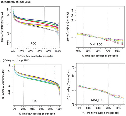
Figure 4. (a) FDC and (b) MM_FDC in catchments with small SFDC, (c) FDC and (d) MM_FDC in catchments with large SFDC.

4.2 FDC portions in comparison to the MM_FDC

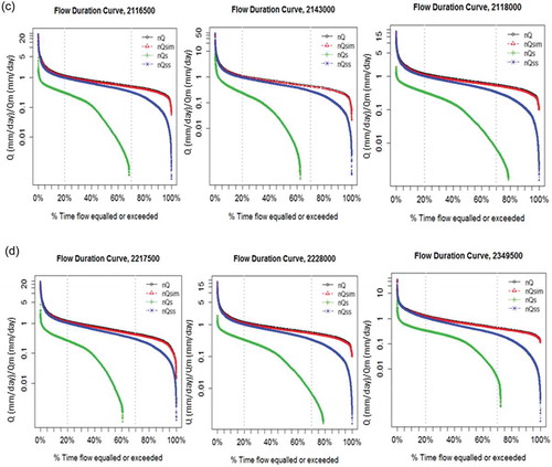
With regard to the upper third of the FDC, we do not observe a difference in the shape of the MM_FDC between both categories of flow variability (Fig. 5). The changes in shape of the upper third of the FDC are explained by the shape of surface and subsurface flow FDCs that track the total flow FDC (Fig. 6). In the upper third, the surface flow and subsurface flow FDCs are steeper in catchments with large flow variability (Fig. 6(a) and (b)) compared to those with small flow variability (Fig. 6(c) and (d)).

Figure 5. Normalized flow (nQ) and normalized MM_FDCs (nQ_reg): (a) and (b) nQ and nQ_reg in catchments with steeper slope of the FDC, (c) and (d) nQ and nQ_reg in catchments with flatter slope of the FDC. The curves were normalized by the mean annual daily flow.

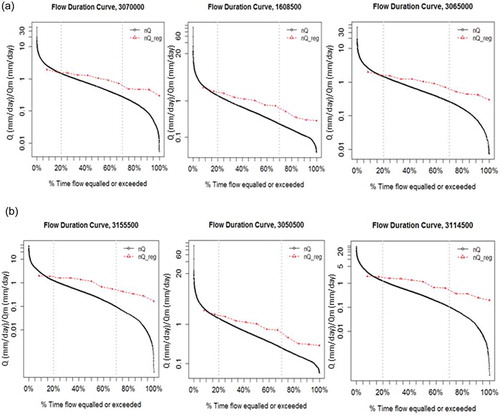
Figure 5. (Continued)

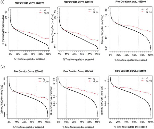
Figure 6. Normalized flow (nQ), normalized simulated flow (nQsim), normalized surface flow (nQs) and normalized subsurface flow (nQss) in catchments with: (a) and (b) steeper FDC, and (c) and (d) flatter FDC. The curves were normalized by the mean annual daily flow.

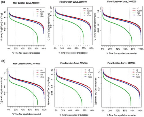
Figure 6. (Continued)

In the middle third of the FDC, we found that the MM_FDCs deviate from the FDCs in catchments with large flow variability (steeper slope of the FDC) and track the FDCs in catchments with small flow variability (flatter slope of the FDC) (Fig. 5). In this portion of the FDC, we find that the surface flow FDC dips at lower flow percentiles (80%) in all the study catchments irrespective of their flow variability (Fig. 6). The subsurface flow FDC tracks the total flow FDC in the middle third in all study catchments. The slopes of both curves (SSFDC and SFDC, respectively) are proportional, with a statistically significant correlation (p < 0.05) (Table 2). The slopes of the SSFDCs were larger than SFDCs in both groups of the flow variability (Fig. 7). We note that in some catchments of large SFDCs, the subsurface flow tracks the total flow; the slope of the SSFDC is nearly equal to SFDC (Fig. 7(a)).

Table 2. Correlation between the slopes of subsurface flow FDC and the FDC.

Catchment	R^2	r	p value
Flatter FDC	0.81	0.9	<0.001
Steeper FDC	0.88	0.93	<0.001

Figure 7. Cumulative distribution function (cdf) of the SFDC and the SSFDC slopes in catchments with (a) steeper FDCs and (b) flatter FDCs.

In the lower third, the MM_FDC deviates from the FDC regardless of the level of flow variability (Fig. 5). The catchments with smaller SFDC have sharper change in slope than those with larger SFDC (Fig. 5(a) and (b) vs Fig. 5(c) and (d)). In the lower third, the subsurface flow FDC displays differences in shape between categories of flow variability (Fig. 6(a) and (b) vs Fig. 6(c) and (d)).

5 Discussion

5.1 Interpretation of the FDC portions in comparison to the MM_FDC

5.1.1 FDC upper third

The upper third of the FDC comprises the largest flows. The MM_FDC diverged from the FDC upper third independently of the value of flow variability (flatter/steeper slope of the FDC). The MM_FDC did not help to differentiate between FDC upper thirds in catchments with different categories of flow variability (Fig. 5). Therefore, it is not possible to use the MM_FDC in predictions of the upper third of the FDC. The shape of FDC upper third is explained using the surface and subsurface flow FDCs (Fig. 6). In this range of flows (Q0% > Q > Q33%), the shapes of FDC that can be distinguished between different categories of flow variability illustrate the effect of the antecedent moisture condition (AMC) dynamics, in the subsurface, in combination with the soil hydraulic properties and the pattern of extreme precipitation. Atieh et al. (2017) showed recently that precipitation is among the most influential parameters in the shape of the FDC, including the upper third. We acknowledge that the effect of AMC dynamics and the soil hydraulic properties on extreme precipitation encapsulate the controls of the catchment response, namely, land cover, catchment geomorphology and topography (e.g. shape, Strahler order and slope). In fact, the land cover conditions influence the infiltration conditions of the soil surface and, therefore, the moisture conditions (Niehoff et al. 2002). This is due to linkages between the land cover, soil macroporosity and unsaturated zone dynamics controlling the infiltration excess runoff mechanism(Niehoff et al. 2002). Moreover, the subsurface flows play a role in the soil moisture redistribution between storm events and in setting up the initial wetness conditions that govern the streamflow generation of subsequent rain events. A dominant control of the impact of subsurface flows on the moisture redistribution is the local topography (Wood et al. 1990). The redistribution of moisture between storm events led us to emphasize the effect of storm seasonality (pattern of change in the seasonal behaviour of storms) in addition to the effect of the magnitude and frequency of extreme precipitation.

In the upper third of the FDC, the effect of AMC dynamics is more likely to be pronounced in catchments of low flow variability, given the flatter shape of flow component FDCs (surface and subsurface flow FDCs in Fig. 6). This is a hypothesis that requires further testing. In these catchments of low flow variability, the soil is well drained (Chouaib et al. 2018). Physically, the larger the infiltration rate, the more likely the rainwater will infiltrate and overland flow will take place as a result of saturation excess runoff mechanisms. With this effect, more changes in the AMC will be visible. The larger infiltration rates delay the soil saturation; the saturation excess mechanism becomes prevalent over the infiltration excess mechanism (Weiler and Naef 2003). The effects of the runoff generation mechanisms on high flows were analysed by Sivapalan et al. (1990) and tested within a stochastic framework. The surface runoff generation mechanisms (saturation excess and infiltration excess overland flow) influence flood frequency shapes research (e.g. Sivapalan et al. 1990). This is a first step towards further analysing whether limited flow variability and predominant saturation excess overland flow flattens the upper third of the FDC. Consequently, predictions of high flows have to account for the effect of AMC that should vary between the storms of particular seasonality specific to the study region. Note that, as shown in Chouaib et al. (2018), the eastern USA portrays a systematic variation in the seasonality of storm events from northeast to the southeast. The storm seasonality and the effect of the between storms timing on high flows was analysed by Sivapalan et al. (2005). The AMC dynamics effect has been underscored in several studies investigating streamflow predictions within a deterministic framework (e.g. Kirchner 2009). Notably, isotope hydrology studies showed the large contribution of pre-event water to the hydrograph compared to event water (e.g. Buttle 1994, Uhlenbrook and Leibundgut 2002). These findings from other studies support the claim about AMC dynamics affecting the upper third of the FDC. Muneepeerakul et al. (2010) showed that surface flow FDC can be derived from the precipitation. In our study, based on findings on the upper third FDCs, the flow component properties and the physical explanations from previous studies, we conjecture that the derivation of large flows should not only use a simple function of precipitation but also account for the AMC effect.

5.1.2 FDC middle third

The MM_FDC diverged from the middle third of the FDC in catchments with steeper SFDC (Fig. 5(a) and (b)), with larger root mean square error (RMSE; Sorooshian et al. 1993), as shown in Table 3. However, the MM_FDC tracked the middle third of the FDC in catchments with flatter SFDC (Fig. 5(c) and (d); smaller RMSE in Table 3). Therefore, it is possible to use the MM_FDC to predict the middle third of the FDC only in catchments with low flow variability. These findings can be further understood from differences in the catchment characteristics and runoff processes between categories of flow variability.

Table 3. RMSE between the slope of the FDC and that of the MM_FDC for the two catchments category.

	RMSE
Flatter FDC	1.69
Steeper FDC	0.99

In the middle third of the FDC (Q33% > Q > Q66%), the surface flow effect on the response was maintained irrespective of the value of flow variability (the surface flow FDC extends to lower flow percentiles, 80%; Fig. 6). Thus, surface and subsurface flow FDCs jointly affect the flow variability. Previous studies have demonstrated that surface runoff is dominant in the rising limb of the hydrograph and to a lesser extent in the falling limb (McDonnell 2003), which further explains the interaction between surface and subsurface flow in this part of the FDC. The subsurface flow FDC displays the effect of subsurface processes, namely deep percolation and evapotranspiration (e.g. Botter et al. 2009). The steeper slope of the subsurface flow FDC compared to that of the total flow FDC, though they are proportional (Table 2), suggests that the subsurface flow response is more sensitive to the effect of subsurface processes than total flow (Fig. 7).

Given the complex combined effect of surface and subsurface flow in this range of the FDC, the mean monthly runoff did not fully capture the variation of the FDC slopes across the study catchments. The SMM_FDC explains only 38% of the total variation of SFDC in the study area (Fig. 3(c)). In catchments with low flow variability, it appears that the differences between high and low flows of the mean monthly runoff – used to calculate the SMM_FDC – can approximate the value of flow variability that is dominated by the effect of both surface and subsurface flow processes.

In catchments with high flow variability, the slopes of the subsurface flow FDCs are larger than their values in catchments with low flow variability (Fig. 7(a) and (b)). In these catchments of steep SFDC, Chouaib et al. (2018) found that subsurface stormflow is predominant. According to Fig. 7(a), some catchments have equivalent slopes of FDC and subsurface flow FDC; these are mountainous and forested catchments. In these mountainous and forested conditions, most likely the surface and subsurface flows are equally dominant. Therefore, they cannot be differentiated in terms of runoff generation mechanisms, which explain the subsurface flow variability being nearly equal to the total flow variability. McDonnell (2013) considered that the lateral connectivity in the subsurface zone increases with increasing catchment slope. The lateral connectivity is larger in catchments in hillslopes and fosters patches of saturation, which makes surface and subsurface runoff generation mechanisms less distinguishable.

It appears that the interaction between surface and subsurface flow yielding the total flow variability cannot be represented by the mean monthly runoff in catchments with steeper slope of the FDC. The differences between the high and low flows from the mean monthly runoff used in SMM_FDC are not helping to predict the real flow variability; monthly averaging attenuates the flow response and masks the behaviour of the flow regime when expressed as FDC.

5.1.3 FDC lower third

The lower third of the FDC is the range of low flows and limited precipitation where the evapotranspiration (ET) effect is dominant (Vitvar et al. 2002).

The MM_FDC diverged from the FDC lower third independently from the value of the flow variability (flatter/steeper slope of the FDC). The MM_FDC did not help to mimic the differences of FDC lower thirds in all study catchments. It is, therefore, not possible to use the MM_FDC in predictions of the lower third of the FDC. This can be further understood by explaining FDC lower thirds between categories of flow variability.

Provided that the FDC has a sharp dip in catchments with high flow variability and a flatter dip in catchments with low flow variability (Fig. 6), it appears that the dominant effect of ET on low flows (lower third of FDC) changes with the catchment flow variability (steeper vs flatter slope of the FDC) and so with their respective landscape properties. Note that Chouaib et al. (2018) found that in the eastern USA all mountainous catchments have smaller soil moisture storage capacity (SMSC) (<280 mm) and all lowland catchments have larger SMSC (>280 mm) independently from the flow variability.

In catchments with steeper SFDC (high flow variability), the ET effect on low flows was not discernible between total and subsurface flow FDCs as both had a sharp dip (Fig. 6(a) and (b)). In this category, all catchments have limited infiltration rates (HGC predominant; Fig. 1(b)). The sharp dips of subsurface and total flow FDCs suggest that the conditions limited infiltration rates in large/small SMSCs is a chief regulator of the influence of ET on the lower third of the FDC.

In catchments with low flow variability, the subsurface flow had a flatter dip than the total flow. The subsurface flow is then more sensitive to the effect of ET at the lower third. The subsurface zone is where the rain water infiltrates and the infiltration rates change non-linearly with depth (Ameli et al. 2016). The improved soil drainage in these catchments of large/small SMSC and the non-linear change of infiltration with depth explains the ET effect and hence the flatter shape of subsurface and total flow FDCs at the lower tail.

In a forested catchment of steep slope in British Columbia, Canada, Moore (1997) demonstrated that at early stages, after a storm event, when the catchment is wetted, the hydrograph recession limb is exponential (linear). However, at later stages, as the drainage from the upslope zones or the recharge from the vadose zone starts, the recession limb becomes non-linear and fits better to a power law function. The two stages of the recession could not be distinguished in the absence of the ET (e.g. during dormant season) (Moore 1997). This explanation of the hydrograph recession limb explains further the effect of ET on low flows and demonstrates that it is one of the major factors making low flows prediction non-linear and highly affected by the catchment characteristics (the soil infiltration rates and the soil storage characteristics). The studies by Botter et al. (2009, 2010) are consistent with the findings of Moore (1997) regarding the non-linear aspect of low flows. Botter et al. (2009, 2010) showed that in conditions of humid climate in northern Italy, the prediction of FDC from the probability of observing the water volume in the subsurface zone provided a more accurate assessment of low flow when the power law (non-linear) is fitted instead of the exponential distribution (linear). This understanding supports our claim about the FDC lower tail and explains the diverging MM_FDC at the lower third irrespective of the value of flow variability. The averaging in the mean monthly runoff does not capture the non-linearity in the low flow response caused primarily by ET, but also to episodic drought conditions. The ET impact changed with properties of the soil infiltration rates in condition of small/large SMSC.

5.2 Catchments and flow conditions to predict the FDC using the MM_FDC

The meta-analysis of the FDCs and the MM_FDCs based on differences in the flow variability showed that FDC prediction using the MM_FDC is only partially applicable. Given the effect of averaging in the mean monthly runoff that smoothes the flow response, the method is limited to specific characteristics of flow variability (flatter vs steeper slope of the FDC) and landscape properties. Chouaib et al. (2018) found that catchments with flatter SFDC are mostly dominated by saturation excess overland flow, whereas those with steeper SFDC are mostly dominated by subsurface stormflow.

In catchments with flatter slope of the FDC, the findings suggest that MM_FDC can be used to predict medium flows; that is, the middle third of the FDC but not the upper and lower thirds. In these catchments, the middle third of the MM_FDC should be able to represent the full range of flows (a portion of fast and slow flows). The catchments in this category have well-drained soils (Fig. 1(a)); few are mountainous and most are located in lowland areas of predominant saturation excess overland flow (Fig. 3(a)).

In catchments with steeper slope of the FDC, it does not appear that FDC portions can be predicted from the MM_FDC, including the middle third. In these catchments the soil is poorly drained (Fig. 1(a)) and most are located in highland areas (Fig. 2(a)) of predominant subsurface stormflow. Few catchments are in lowlands with poorly drained soils (Fig. 2(a)).

The MM_FDC slopes were smaller than those of the FDCs. Thus, even when it is possible to use MM_FDC to predict FDC, the simulated middle third of the FDC might be used as indicative rather than a firm estimation.

Our findings partially agree with the theoretical study of Yokoo and Sivapalan (2011), who suggested that the middle and lower thirds of the FDC can be estimated by mean monthly runoff in catchments with perennial streamflow and humid climate. The method is constrained by the value of flow variability and is applicable only for the middle third of the FDC. The upper third prediction should involve non-linear filtering of the precipitation that has to account for the AMC effect on large flows. The high flow predictions should include the surface flow and a portion of the slow flows.

At the lower third, the FDC predictions ought to consider the non-linear effect of ET on low flows. The ET effect may be studied in future investigations by simulating the dynamics of the saturated area near the stream during low flows (Yokoo and Sivapalan 2011).

The meta-analysis in real catchments and the large dataset made our results complementary to the findings from using a hypothetical catchment. The regional scale helped to combine a wide range of flow response properties with complexity in the physiography of real catchments. Analysis of observed flows and simulated flow components allowed us to reveal facets about the use of MM_FDC not explored within the context of a theoretical study. Future research may extend our work and investigate the use of monthly FDCs to predict FDCs in ungauged catchments.

5.3 Conceptual model of the FDC and MM_FDC

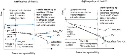
The outcomes of the meta-analysis are summarized in a conceptual illustrative model of the FDC in relation to the MM_FDC shown in Fig. 8. The conceptual model states hypotheses about controls of the FDC portions and predictions using the MM_FDC. The findings will serve as guidance for future studies to develop a physically based prediction model of the FDC in ungauged catchments. The shapes of FDC that are distinguished between different categories of flow variability illustrate the effect of the AMC dynamics and other factors, namely, the soil hydraulic properties, the extreme precipitation magnitudes and patterns of the storm seasonality. The upper and the middle thirds of the FDC are controlled by the subsurface and surface flow. In catchments with flat slope of the FDC, the upper third is flatter due to the effect of well-drained soils and predominant saturation excess overland flow in most of the catchments. The middle third of the FDC can be represented by the MM_FDC. For the lower third, the subsurface flow is more sensitive to the ET effect than the total flow. The subsurface flow FDC has a flatter dip than the total flow FDC due to large soil infiltration rates in catchments of large/small SMSCs (Fig. 8(a)). The MM_FDC does not capture the dominant effect of ET during low flows and deviates from FDC at the lower third.

In catchments with steeper FDCs, the upper third is steeper due to the effect of poorly drained soils and predominant subsurface stormflow in most of the catchments, while the middle third is very steep and cannot be represented by the MM_FDC. The subsurface flow FDC and FDC overlap and have equal slopes in the steepest mountainous catchments. At the lower third, the subsurface flow and total flow are equally sensitive to the ET effect, where both have a sharp dip irrespective of the value of the SMSC (Fig. 8(b)). The MM_FDC does not capture the dominant effect of ET during low flows and deviates from the FDC at the lower third.

Figure 8. Conceptual model of the FDC in conditions of humid climate and perennial runoff in catchments with (a) flatter FDCs and (b) steeper FDCs. AMC: antecedent moisture conditions.

6 Conclusions

This study sought to investigate the catchment and climate conditions under which the mean monthly runoff, represented in the stochastic form of the FDC (MM_FDC), can be used to predict the FDC. This investigation is an initial step in gaining understanding to quantify the FDC in ungauged catchments following a physically based approach and more readily available monthly flow data. The mean monthly flows are available from predictions of global models and/or from regionalization methods. The study used the data of 73 catchments from the eastern USA, where the climate is humid and the precipitation is of limited seasonality. In these catchments of perennial runoff, the results show that it is applicable to use the MM_FDC in predicting the middle third of the FDC. However, the MM_FDC does not distinguish the shapes of the upper or lower thirds dominated by the varying effect of antecedent moisture conditions and the effect of evapotranspiration, respectively. The averaging in the mean monthly runoff smoothes the flow response. Our results show that the use of MM_FDC to predict the middle third of the FDC is primarily constrained by the characteristics of the flow variability and landscape properties. Only in catchments of low flow variability (flatter slope of the FDC), could the MM_FDC track the middle third of the FCD. These catchments have mostly predominant saturation excess overland flow in well-drained soils of large SMSC. Few other catchments are mountainous with soils of large infiltration rates and limited SMSC. It is important to recognize that the non-applicability of the method in catchments with steeper SFDC (high flow variability) indicates the complexity of the hydrological response and highlights the scope for future research.

We recommend similar empirical analysis in other regions of different climate and flow characteristics elsewhere in the USA and worldwide. For instance, the precipitation seasonality would have an impact when compared to seasonality of the ET (being in phase vs out of phase) given the dominant effect of ET during low flow periods. Our empirical study can be aided by numerical experiments to test the several hypotheses and investigate a prediction model of the FDC using the MM_FDC under several complex combinations of real climate and physiographic conditions. These future empirical and numerical analyses will provide the opportunity to refute or corroborate our conclusions and get more evidence about the use of MM_FDC. Our study is limited in revealing the effect of non-stationarity to make predictions of the FDC using the MM_FDC. The non-stationarity in the study catchments is mainly caused by the climate variability because the anthropogenic activity is limited. Our conclusions may not hold in the future under non-stationarity caused by future anthropogenic climate or land-use change. Despite the limitations, the understanding we gained helped to provide an illustrative conceptual model of the FDC in relation to the MM_FDC, which will serve for future works investigating process-based methods to predict FDC in ungauged catchments.

Acknowledgements

We thank the two anonymous reviewers for their careful reading of our manuscript and their many insightful comments and suggestions. We thank the associate editor for their feedback that helped to improve the quality of the manuscript.

Disclosure statement

No potential conflict of interest was reported by the authors.

Additional information

Funding

W. Chouaib is grateful for the Islamic Development Bank (IDB) who funded her PhD studies at the University of British Columbia. This study was partially funded by internal awards of the Faculty of Forestry: Weldwood of Canada Limited H. Richard Whittall, 2016, Mary and David Macaree, 2015 and Peter Rennie Memorial Award, 2017, and the NSERC – Canada Discovery Grant to Dr Younes Alila [RGPIN 194388-11].

References

- Ameli, A.A., Craig, J.R., and McDonnell, J.J., 2015. Are all runoff processes the same? Numerical experiments comparing a Darcy‐Richards solver to an overland flow‐based approach for subsurface storm runoff simulation. Water Resources Research, 51 (12), 10008–10028. doi:10.1002/2015WR017199
- Ameli, A.A., McDonnell, J.J., and Bishop, K., 2016. The exponential decline in saturated hydraulic conductivity with depth: a novel method for exploring its effect on water flow paths and transit time distribution. Hydrological Processes, 30 (14), 2438–2450. doi:10.1002/hyp.v30.14
- Atieh, M., et al., 2017. Prediction of flow duration curves for ungauged basins. Journal of Hydrology, 545, 383–394. doi:10.1016/j.jhydrol.2016.12.048
- Barthold, F.K. and Woods, R.A., 2015. Stormflow generation: a meta‐analysis of field evidence from small, forested catchments. Water Resources Research, 51 (5), 3730–3753. doi:10.1002/2014WR016221
- Berghuijs, W.R., et al., 2014. Patterns of similarity of seasonal water balances: a window into streamflow variability over a range of time scales. Water Resources Research, 50 (7), 5638–5661. doi:10.1002/2014WR015692
- Beven, K., 1989. Changing ideas in hydrology—the case of physically-based models. Journal of Hydrology, 105 (1–2), 157–172. doi:10.1016/0022-1694(89)90101-7
- Beven, K., 2000. On the future of distributed modelling in hydrology. Hydrological Processes, 14 (16‐17), 3183–3184. doi:10.1002/1099-1085(200011/12)14:16/17<3183::AID-HYP404>3.0.CO;2-K
- Blöschl, G., et al., eds. 2013. Runoff prediction in ungauged basins: synthesis across processes, places and scales. Cambrigdem, UK: Cambridge University Press.
- Booker, D.J. and Snelder, T.H., 2012. Comparing methods for estimating flow duration curves at ungauged sites. Journal of Hydrology, 434, 78–94. doi:10.1016/j.jhydrol.2012.02.031
- Botter, G., et al., 2007a. Basin‐scale soil moisture dynamics and the probabilistic characterization of carrier hydrologic flows: slow, leaching‐prone components of the hydrologic response. Water Resources Research, 43 (2). doi:10.1029/2006WR005043
- Botter, G., et al., 2007b. Probabilistic characterization of base flows in river basins: roles of soil, vegetation, and geomorphology. Water Resources Research, 43 (6). doi:10.1029/2006WR005397
- Botter, G., et al., 2009. Nonlinear storage‐discharge relations and catchment streamflow regimes. Water Resources Research, 45 (10), W10427. doi:10.1029/2008WR007658
- Botter, G., et al., 2010. Natural streamflow regime alterations: damming of the Piave river basin (Italy). Water Resources Research, 46 (6), W06522. doi:10.1029/2009WR008523
- Buttle, J.M., 1994. Isotope hydrograph separations and rapid delivery of pre-event water from drainage basins. Progress in Physical Geography, 18 (1), 16–41. doi:10.1177/030913339401800102
- Castellarin, A., et al., 2004. Regional flow-duration curves: reliability for ungauged basins. Advances in Water Resources, 27 (10), 953–965. doi:10.1016/j.advwatres.2004.08.005
- Castellarin, A., et al. 2013. Prediction of flow duration curves in ungauged basins. Chapter 7. In: G. Blöschl, ed. Runoff prediction in ungauged basins: synthesis across processes, places and scales. Cambridge, UK: Cambridge University Press, 135–162.
- Castellarin, A., 2014. Regional prediction of flow–duration curves using a three-dimensional kriging. Journal of Hydrology, 513, 179–191. doi:10.1016/j.jhydrol.2014.03.050
- Castellarin, A., et al., 2018. Prediction of streamflow regimes over large geographical areas: interpolated flow–duration curves for the Danube region. Hydrological Sciences Journal, 63 (6), 845–861. doi:10.1080/02626667.2018.1445855
- Ceola, S., et al., 2010. Comparative study of ecohydrological streamflow probability distributions. Water Resources Research, 46 (9), W09502. doi:10.1029/2010WR009102
- Chouaib, W., Caldwell, P.V., and Alila, Y., 2018. Regional variation of flow duration curves in the eastern USA: process-based analyses of the interaction between climate and landscape properties. Journal of Hydrology, 559, 327–346. doi:10.1016/j.jhydrol.2018.01.037
- Claps, P. and Fiorentino, M., 1997. Probabilistic flow duration curves for use in environmental planning and management. Integrated approach to environmental data management systems. NATO-ASI Series, 2 (31), 255–266.
- Coopersmith, E., et al., 2012. Exploring the physical controls of regional patterns of flow duration curves–Part 3: a catchment classification system based on regime curve indicators. Hydrology and Earth System Sciences, 16 (11), 4467–4482. doi:10.1029/2010WR009286
- Duan, Q., et al., 2006. Model Parameter Estimation Experiment (MOPEX): an overview of science strategy and major results from the second and third workshops. Journal of Hydrology, 320 (1), 3–17. doi:10.1016/j.jhydrol.2005.07.031
- Evaristo, J. and McDonnell, J.J., 2017. Prevalence and magnitude of groundwater use by vegetation: a global stable isotope meta-analysis. Scientific Reports, 7, 44110. doi:10.1038/srep44110
- Feser, F., et al., 2011. Regional climate models add value to global model data: a review and selected examples. Bulletin of the American Meteorological Society, 92 (9), 1181–1192. doi:10.1175/2011BAMS3061.1
- Ganora, D., et al., 2009. An approach to estimate nonparametric flow duration curves in ungauged basins. Water Resources Research, 45 (10), W10418. doi:10.1029/2008WR007472
- Grayson, R.B., et al., 2002. Advances in the use of observed spatial patterns of catchment hydrological response. Advances in Water Resources, 25 (8–12), 1313–1334. doi:10.1016/S0309-1708(02)00060-X
- Greenland, S., Lash, T.L., and Rothman, K.J., 2008. Modern epidemiology. Philadelphia, PA: Lippincott Williams & Wilkins, 283–302.
- Holmes, M.G.R., et al., 2002. A region of influence approach to predicting flow duration curves within ungauged catchments. Hydrology and Earth System Sciences Discussions, 6 (4), 721–731. doi:10.5194/hess-6-721-2002
- Hrachowitz, M., et al., 2013. A decade of predictions in ungauged basins (PUB)—a review. Hydrological Sciences Journal, 58 (6), 1198–1255. doi:10.1080/02626667.2013.803183
- Kirchner, J.W., 2009. Catchments as simple dynamical systems: catchment characterization, rainfall‐runoff modeling, and doing hydrology backward. Water Resources Research, 45 (2), W02429. doi:10.1029/2008WR006912
- Klemeš, V., 1983. Conceptualization and scale in hydrology. Journal of Hydrology, 65 (1–3), 1–23. doi:10.1016/0022-1694(83)90208-1
- LeBoutillier, D.W. and Waylen, P.R., 1993. A stochastic model of flow duration curves. Water Resources Research, 29 (10), 3535–3541. doi:10.1029/93WR01409
- McDonnell, J.J., 2003. Where does water go when it rains? Moving beyond the variable source area concept of rainfall–runoff response. Hydrological Processes, 17 (9), 1869–1875. doi:10.1002/(ISSN)1099-1085
- McDonnell, J.J., 2013. Are all runoff processes the same? Hydrological Processes, 27 (26), 4103–4111. doi:10.1002/hyp.v27.26
- Merheb, M., et al., 2016. Hydrological response characteristics of mediterranean catchments at different time scales: a meta-analysis. Hydrological Sciences Journal, 61 (14), 2520–2539. doi:10.1080/02626667.2016.1140174
- Moore, R.D., 1997. Storage-outflow modeling of streamflow recessions, with application to a shallow-soil forested catchment. Journal of Hydrology, 198 (1), 260–270. doi:10.1016/S0022-1694(96)03287-8
- Muneepeerakul, R., et al., 2010. Daily streamflow analysis based on a two‐scaled gamma pulse model. Water Resources Research, 46 (11), W11546. doi:10.1029/2010WR009286
- Nash, J.E. and Sutcliffe, J.V., 1970. River flow forecasting through conceptual models part I—A discussion of principles. Journal of Hydrology, 10 (3), 282–290. doi:10.1016/0022-1694(70)90255-6
- Niehoff, D., Fritsch, U., and Bronstert, A., 2002. Land-use impacts on storm-runoff generation: scenarios of land-use change and simulation of hydrological response in a meso-scale catchment in SW-Germany. Journal of Hydrology, 267 (1–2), 80–93. doi:10.1016/S0022-1694(02)00142-7
- Nijssen, B., et al., 2001. Predicting the discharge of global rivers. Journal of Climate, 14 (15), 3307–3323. doi:10.1175/1520-0442(2001)014<3307:PTDOGR>2.0.CO;2
- Poff, N.L., et al., 1997. The natural flow regime. BioScience, 47 (11), 769–784. doi:10.2307/1313099
- Prudhomme, C., Reynard, N., and Crooks, S., 2002. Downscaling of global climate models for flood frequency analysis: where are we now? Hydrological Processes, 16 (6), 1137–1150. doi:10.1002/(ISSN)1099-1085
- Pugliese, A., et al., 2016. Regional flow duration curves: geostatistical techniques versus multivariate regression. Advances in Water Resources, 96, 11–22. doi:10.1016/j.advwatres.2016.06.008
- Razavi, T. and Coulibaly, P., 2012. Streamflow prediction in ungauged basins: review of regionalization methods. Journal of Hydrologic Engineering, 18 (8), 958–975. doi:10.1061/(ASCE)HE.1943-5584.0000690
- Requena, A.I., Ouarda, T.B., and Chebana, F., 2018. Low-flow frequency analysis at ungauged sites based on regionally estimated streamflows. Journal of Hydrology, 563, 523–532. doi:10.1016/j.jhydrol.2018.06.016
- Sauquet, E. and Catalogne, C., 2011. Comparison of catchment grouping methods for flow duration curve estimation at ungauged sites in France. Hydrology and Earth System Sciences, 15 (8), 2421. doi:10.5194/hess-15-2421-2011
- Sawicz, K., et al., 2011. Catchment classification: empirical analysis of hydrologic similarity based on catchment function in the eastern USA. Hydrology and Earth System Sciences, 15 (9), 2895–2911. doi:10.5194/hess-15-2895-2011
- Singh, R.D., Mishra, S.K., and Chowdhary, H., 2001. Regional flow-duration models for large number of ungauged Himalayan catchments for planning microhydro projects. Journal of Hydrologic Engineering, 6 (4), 310–316. doi:10.1061/(ASCE)1084-0699(2001)6:4(310)
- Sivapalan, M., et al., 2003. Downward approach to hydrological prediction. Hydrological Processes, 17 (11), 2101–2111. doi:10.1002/hyp.v17:11
- Sivapalan, M., et al., 2005. Linking flood frequency to long‐term water balance: incorporating effects of seasonality. Water Resources Research, 41 (6). doi:10.1029/2004WR003439
- Sivapalan, M., Wood, E.F., and Beven, K.J., 1990. On hydrologic similarity: 3. A dimensionless flood frequency model using a generalized geomorphologic unit hydrograph and partial area runoff generation. Water Resources Research, 26 (1), 43–58.
- Smakhtin, V.Y., Hughes, D.A., and Creuse-Naudin, E., 1997. Regionalization of daily flow characteristics in part of the Eastern Cape, South Africa. Hydrological Sciences Journal, 42 (6), 919–936. doi:10.1080/02626669709492088
- Sood, A. and Smakhtin, V., 2015. Global hydrological models: a review. Hydrological Sciences Journal, 60 (4), 549–565. doi:10.1080/02626667.2014.950580
- Sorooshian, S., Duan, Q., and Gupta, V.K., 1993. Calibration of rainfall‐runoff models: application of global optimization to the sacramento soil moisture accounting model. Water Resources Research, 29 (4), 1185–1194. doi:10.1029/92WR02617
- Uhlenbrook, S. and Leibundgut, C., 2002. Process‐oriented catchment modelling and multiple‐response validation. Hydrological Processes, 16 (2), 423–440. doi:10.1002/(ISSN)1099-1085
- Vandewiele, G.L. and Elias, A., 1995. Monthly water balance of ungauged catchments obtained by geographical regionalization. Journal of Hydrology, 170 (1–4), 277–291. doi:10.1016/0022-1694(95)02681-E
- Vitvar, T., et al., 2002. Estimation of baseflow residence times in watersheds from the runoff hydrograph recession: method and application in the Neversink watershed, Catskill Mountains, New York. Hydrological Processes, 16 (9), 1871–1877. doi:10.1002/(ISSN)1099-1085
- Vogel, R.M. and Fennessey, N.M., 1994. Flow-duration curves. I: new interpretation and confidence intervals. Journal of Water Resources Planning and Management, 120 (4), 485–504. doi:10.1061/(ASCE)0733-9496(1994)120:4(485)
- Vogel, R.M. and Fennessey, N.M., 1995. Flow duration curves II: a review of applications in water resources planning. JAWRA Journal of the American Water Resources Association, 31 (6), 1029–1039. doi:10.1111/jawr.1995.31.issue-6
- Weiler, M. and Naef, F., 2003. An experimental tracer study of the role of macropores in infiltration in grassland soils. Hydrological Processes, 17 (2), 477–493. doi:10.1002/(ISSN)1099-1085
- Wood, E.F., Sivapalan, M., and Beven, K., 1990. Similarity and scale in catchment storm response. Reviews of Geophysics, 28 (1), 1–18. doi:10.1029/RG028i001p00001
- Wood, M.K. and Blackburn, W.H., 1984. An evaluation of the hydrologic soil groups as used in the SCS runoff method on rangelands. Journal of the American Water Resources Association, 20 (3), 379–389. doi:10.1111/jawr.1984.20.issue-3
- Xie, P. and Arkin, P.A., 1996. Analyses of global monthly precipitation using gauge observations, satellite estimates, and numerical model predictions. Journal of Climate, 9 (4), 840–858. doi:10.1175/1520-0442(1996)009<0840:AOGMPU>2.0.CO;2
- Yadav, M., Wagener, T., and Gupta, H., 2007. Regionalization of constraints on expected watershed response behavior for improved predictions in ungauged basins. Advances in Water Resources, 30 (8), 1756–1774. doi:10.1016/j.advwatres.2007.01.005
- Yaeger, M., et al., 2012. Exploring the physical controls of regional patterns of flow duration curves–Part 4: A synthesis of empirical analysis, process modeling and catchment classification. Hydrology and Earth System Sciences, 16 (11), 4483–4498. doi:10.5194/hess-16-4483-2012
- Ye, S., et al., 2012. Exploring the physical controls of regional patterns of flow duration curves–Part 2: Role of seasonality, the regime curve, and associated process controls. Hydrology and Earth System Sciences, 16 (11), 4447–4465. doi:10.5194/hess-16-4447-2012
- Yokoo, Y. and Sivapalan, M., 2011. Towards reconstruction of the flow duration curve: development of a conceptual framework with a physical basis. Hydrology and Earth System Sciences, 15 (9), 2805–2819. doi:10.5194/hess-15-2805-2011
- Zhang, Z., et al., 2008. Reducing uncertainty in predictions in ungauged basins by combining hydrologic indices regionalization and multiobjective optimization. Water Resources Research, 44 (12), 44, W00B04. doi:10.1029/2008WR006