Revealing hidden persistence in maximum rainfall records

ABSTRACT

Clustering of extremes is critical for hydrological design and risk management and challenges the popular assumption of independence of extremes. We investigate the links between clustering of extremes and long-term persistence, else Hurst-Kolmogorov (HK) dynamics, in the parent process exploring the possibility of inferring the latter from the former. We find that (a) identifiability of persistence from maxima depends foremost on the choice of the threshold for extremes, the skewness and kurtosis of the parent process, and less on sample size; and (b) existing indices for inferring dependence from series of extremes are biased downward when applied to non-Gaussian processes. We devise a probabilistic index based on the probability of occurrence of peak-over-threshold events across multiple scales, which can reveal clustering, linking it to the persistence of the parent process. Its application shows that rainfall extremes may exhibit noteworthy departures from independence and consistency with an HK model.

KEYWORDS:

• extremes
• clustering
• HK dynamics
• persistence
• peaks over threshold
• rainfall

Editor A. Castellarin Associate editor E. Volpi

1 Introduction

The identification of clusters in series of extreme events is an ongoing research topic in geosciences, including hydrology, one that is particularly challenging due to the large estimation uncertainties involved when studying series of rare events. Regardless of the complications, this question has multiple important implications for earth sciences which range from understanding natural variability and process dynamics to correctly applying stochastic models for the purposes of inference and prediction. This is evident as most relevant hydrological and engineering applications require settling this issue at the early stage of the analysis, by either assuming independence (e.g. Coles et al. 2001, Kottegoda and Rosso 2008) or ‘ensuring’ it through ‘adequate’ sampling techniques (Ferro and Segers 2003). Thereby, the research focus can be uniquely placed on the more straightforward task of characterizing the probability distribution of extremes. For example, typical flood guidelines suggest that successive flood events have at least a certain separation lag time in order to be considered independent for the application of models (Lang et al. 1999). In light of concerns for intensification of hydrological extremes due to anthropogenic forcing, the investigation of clustering receives additional interest (Ntegeka and Willems 2008, Merz et al. 2016, Tye et al. 2019, Serinaldi and Kilsby 2018), as attribution of trends to an external deterministic forcing presupposes that at least the presence of natural inherent variability has been beforehand properly accounted for. In this respect, increasing evidence reporting the presence of persistence in various hydroclimatic variables (Hurst 1951, Koutsoyiannis 2003, Montanari 2003, Markonis and Koutsoyiannis 2016, O’Connell et al. 2016, Iliopoulou et al. 2016, Tegos et al. 2017, Dimitriadis 2017) gives rise to the question of whether or not, and to what extent a regular behaviour of the extremes originating from persistent processes could be misinterpreted as a result of an anthropogenic cause.

This study deals with the investigation of clustering behaviour in records of maxima with a special focus on long-term daily rainfall observational records. As recent studies reported evidence on the presence of persistence in annual rainfall (Iliopoulou et al. 2016, Tyralis et al. 2018), the question of possible propagation of persistence to rainfall extremes naturally arises. Therefore, the research objectives can be articulated as follows: (a) what are the links between persistence in the parent process and clustering of extreme events and can we infer the one from the other? and (b) what constitutes an informative characterization for clustering?

Typically, the assessment of clustering properties of extremes from a time series implies the selection of a threshold based on which the sampling of ‘extreme’ events is performed. Then, clustering is quantified based on the departure of the properties of extremes from the ones of a purely random process. This evaluation is performed either by considering the series of the inter-arrival times of extremes or equivalently, the series of counts of extreme events over counting windows. There is a direct correspondence between the two; it is well-known for example, that when the data come from a Poisson process, their inter-arrival times are exponentially distributed (Papoulis 1991).

In the hydrological literature, various ad-hoc, sometimes visual and subjective approaches are used in order to quantify departures of extremes – typically floods – from independence and characterize clustering. The most systematic usually consist of some type of ‘window’ analysis, where the time series is split into sub-periods which are examined for presence of perturbations in the statistics of extreme events, often corroborated by statistical testing (Ntegeka and Willems 2008, Willems 2013, Marani and Zanetti 2015). Avoiding the need for selection of time windows to study, Merz et al. (2016) applied a dispersion index, although mostly focused on a combination of kernel-based methods coupled with statistical significance tests to identify flood-rich and flood-poor periods in Germany. Yet, with a few exceptions only (Eichner et al. 2011, Serinaldi and Kilsby 2016, 2018), the majority of clustering characterizations for hydrological extremes are not studied in relation to the dependence properties of the parent process, which is the focal point here.

To evaluate the clustering properties in a more comprehensive framework, two established indices are used in geophysical time series analysis, especially for the clustering analysis of earthquakes (Telesca et al. 2002) and storms (Vitolo et al. 2009) and are based on the ‘counts’ approach: the index of dispersion and the Allan factor. Both can be used to formally test the data against the Poissonian assumption (Serinaldi 2013, Serinaldi and Kilsby 2013) and it is reported that their scaling behaviour can also reveal the fractal properties of the underlying process for ideal rate fractal processes (Thurner et al. 1997). The latter is related to the asymptotic dependence property for large time horizons, long-term dependence, quantified by the Hurst parameter. For revealing the Hurst-Kolmogorov (HK) dynamics, a number of methods examining the original series also exist with the climacogram (Koutsoyiannis 2010), i.e. the variance of the aggregated process over scales, shown to be the most robust (Dimitriadis and Koutsoyiannis 2015).

We briefly review the above methods based on their performance on revealing the clustering of extremes sampled from synthetic time series generated in order to exhibit various degrees of persistence and different marginal distributions. We assess their degree of generality and showcase their shortcomings when extremes arrive from complex processes. We show how the interplay of persistence and moments of order higher than 2 (skewness, kurtosis) can obscure the identification of the latter from extremes. Accordingly, we propose an alternative characterization of clustering based on a probabilistic index with distinctive features and test the proposed method on synthetic and real-world rainfall data. We find that the index exhibits some advantageous characteristics, namely it is capable of quantifying clustering by probabilistic means, linking it to the scaling behaviour of the parent process for a range of distributional and dependence properties. It also enables modelling the probabilities of threshold exceedences across multiple timescales, which can be used as a simulation tool, that being an important advance over existing methods that have mainly an inferential character.

2 Dataset

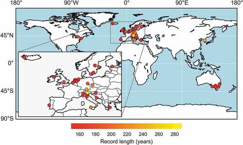
An extended dataset comprising the 60 longest available daily rainfall records is investigated in terms of its extreme properties. The data used in this study are collected from global datasets, i.e. the Global Historical Climatology Network Daily database (Menne et al. 2012) and the European Climate Assessment and Dataset (Klein Tank et al. 2002), and third parties listed in the acknowledgements section. They present an update of the previous dataset explored in Iliopoulou et al. (2018) of long rainfall records surpassing 150 years of daily values. The geographical location of the raingauges is shown in Fig. 1. The length of the time series enables the investigation of clustering on extended time horizons from daily to yearly timescales.

Figure 1. Map of the 60 stations with longest records used in the analysis.

3 Methodological framework

3.1 Definition of notation and mathematical formulation

Let x_i be a stationary stochastic process in discrete time i, i.e. a collection of random variables x_i, and x: = {x₁, … x_n} a single realization (observation) of the latter, i.e. a time series. Now for u being a threshold, u ϵ ℝ, we define the process of peaks over the threshold (POT) consisting of events surpassing the threshold u, i.e.:

(1) ${\underset{\_}{y}}_i:=\left\{\begin{array}{cc}{\underset{\_}{x}}_i,& {\underset{\_}{x}}_i>u\\ 0,& {\underset{\_}{x}}_i\le u\end{array}\right.$(1)

Let also N(t) be a counting process of POT occurrences in time which is an increasing function of time t. We then define the process z^(k)_q:= N(qk)–N((q – 1)k) as the number of occurrences of POT at timescale k and at discrete time q = 1, …, n/k.

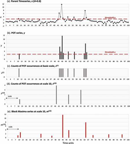
We also define by m^(k)_q:= max_{(q – 1)k ≤ j ≤ qk}{x_j} the block maxima series, which is formed by extracting the maximum order statistic of the observations divided in non-overlapping equally sized periods of length (timescale) k. In the following, we call the timescale k as timescale of filtering of the maxima. Figure 2 visualizes all the above at two temporal scales for a realization of a random process with Hurst parameter H=0.8 and the first four moments following a generalized Pareto distribution.

Figure 2. Explanatory graph of mathematical formulation: (a) Parent time series, (b) POT series, (c) temporal distribution of counts of POT at basic scale k = 1, (d) temporal distribution of counts of POT occurrences at scale k = 10 and (e) block maxima series at scale k = 10.

3.2 Generation of benchmark synthetic time series

To evaluate the ability of clustering indices to discern the dependence characteristics of the parent (extreme generating) process, we first produce a set of synthetic time series x_i with different dependence properties and marginal distributions. For the generation scheme, we employ a simulation procedure proposed by Dimitriadis and Koutsoyiannis (2018), which is capable of generating time series explicitly reproducing chosen theoretical moments up to any order together with any (long-term) persistence structure, i.e. the HK dynamics. We focus here only on processes exhibiting persistence as these are the ones assumed consistent with the natural phenomena studied and also known to produce long-term clustering. For the marginal distribution, we generate time series preserving up to the fourth-order moments following the normal, generalized Pareto and gamma distributions. The higher-order moments of the generated time series follow the entropic distribution. Because the generation scheme preserves up to a specific number of moments from a distribution, the final shape may be slightly distorted with respect to the theoretical one, and therefore, we denote the generated series as type-gamma and type-Pareto, instead of gamma and generalized Pareto, respectively. For a detailed explanation of the generation scheme, the reader is referred to Dimitriadis and Koutsoyiannis (2018). We focus only on the first four moments as higher-order classical moments cannot be reliably estimated from ordinary sample sizes (Lombardo et al. 2014).

The properties of these time series are chosen in order to cover a range of statistical and stochastic characteristics in terms of skewness, kurtosis and H parameter, and therefore, provide a good benchmark sample for testing the indices in typical but also more ‘extreme’ cases. Their properties are summarized in Table 1. We note that these time series are meant as theoretical case studies to test the appropriateness of the indices and are not to be considered as synthetic series of daily rainfall, which are the real-world data in question. However, since only the sequence of counts of extremes is of interest, and not their actual values, it is not necessary to strictly preserve other properties of daily rainfall, i.e. intermittency, and therefore in this sense comparison to the synthetic series is allowed. A sample of the time series is plotted in Fig. 3.

Table 1. Properties of the benchmark samples used in the experiments.

Distribution type	Parameters			Mean	Variance	Skewness	Kurtosis	H	Length
	Shape	Scale	Location
Normal	–	2.6	1.25	1.25	2.6	0	3	0.5–0.99	10^6
Gamma	0.1	5.1	-	0.51	2.6	6.325	63	0.5–0.99	10^6
Gamma	0.01	16.125	-	0.16	2.6	20	603	0.5–0.99	10^6
Pareto	0.1	1	0	1.11	1.54	2.81	17.83	0.5–0.99	10^6
Pareto	0.2	1	0	1.25	2.6	4.65	73.8	0.5–0.99	10^6

Figure 3. Visualization of three time series with H = 0.8 and different marginal distributions generated from the 4-moment SMA scheme (Dimitriadis and Koutsoyiannis 2018). The legends report, respectively, the mean, standard deviation, coefficient of skewness and coefficient of kurtosis of each distribution.

Additionally to the above benchmark time series, we generate ensembles of shorter time series having lengths of 150 × 365 values, i.e. equal to the minimum record length of the rainfall data, and preserving the same moments as the benchmark time series. These series are produced using fewer weights for the SMA scheme, up to 2000, but applying proper weight adjustment scheme (Koutsoyiannis 2016). They reproduce two dependence structures, white noise, and HK with H parameter 0.7, considered a representative value for hydrological processes. The purpose of the second benchmark sample is to test the methods in ‘realistic’ record lengths and to evaluate estimation uncertainty by Monte Carlo simulations that require significantly less computational effort compared to the first benchmark sample, which is generated using 10⁶ weights, i.e. equal to the series length.

3.3 Second-order characterization of extremes

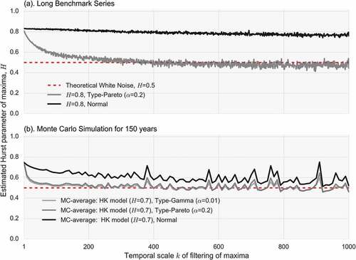
The Hurst parameter is a well-established measure of persistence. It can be estimated from the slope of the double logarithmic plot of the standard deviation of the averaged process vs the averaging timescale, i.e. the climacogram (Koutsoyiannis 2010). To test how the estimator is impacted when extremes are used instead of the original values, we compute the H parameter for extremes extracted from windows (scales) of length 1 to N/10, where N is the time series length. An example is provided in Fig. 4. The first H value (scale = 1) is the value for the original data (the parent time series) and, as the scale increases progressively, the time series is filtered to show only the most ‘extreme’ data. For instance, if the basic timescale is daily, the estimated H parameter at timescale k = 365 corresponds to the H parameter of the annual maxima. To reduce computational time, we perform estimation every 50 scales. The results shown in Fig. 4 are for the normal and the other benchmark time series. The impact of skewness and kurtosis on the estimator is striking as in the case of non-Gaussian time series, the H parameter quickly decays to 0.5, as if there was independence. On the contrary, for the normal time series it yields almost a stable value. To verify that this is not due to the impact of standard deviation bias induced by dependence, we performed estimation for selected timescales with the unbiased with respect to standard deviation, LSSV estimator (Koutsoyiannis 2003, Tyralis and Koutsoyiannis 2011) as well. We also repeat the estimation for the shorter time series and plot the average values at each scale obtained from the Monte Carlo experiments. The same conclusion can be drawn. The climacogram estimator is severely biased downward for extremes originating from non-Gaussian processes and falsely indicates independence after a few scales of filtering. Therefore, we do not consider the climacogram estimator for the rest of the analysis on empirical data. Since it has been shown that the climacogram is closely related to other second-order characterizations, i.e. spectrum and autocovariance (Dimitriadis and Koutsoyiannis 2015), we also expect similar results from the latter. Furthermore, Barunik and Kristoufek (2010) have shown that even for the underlying process (the parent), the sampling properties of the Hurst parameter estimation by some other approaches, i.e. the multifractal detrended fluctuation analysis and the detrending moving average, are also greatly impacted by heavy tails.

Figure 4. H parameters estimated from block maxima series at increasing scale of filtering for (a) benchmark series of length 10⁶ from HK models with H = 0.8 following normal and type-Pareto distributions, and (b) average H values from 10³ Monte Carlo simulations for HK models with H = 0.7 and three different marginal distributions, type-gamma, type-Pareto and normal.

3.4 Clustering indices: the dispersion index

A well-known measure of clustering of events is the index of dispersion of counts, also known as the Fano factor (e.g. Thurner et al. 1997), which is defined as the ratio of the variance of the counts of events vs their mean number at a specific timescale k, i.e.:

(2) ${\underset{\_}{d}}^{\left(k\right)}=\frac{\mathrm{E}\left[{\underset{\_}{z}}_k^2\right]-E{\left[{\underset{\_}{z}}_k\right]}^2}{\mathrm{E}\left[{\underset{\_}{z}}_k\right]}$(2)

For a Poisson point process, the dispersion index is unity for all timescales. According to the literature (Thurner et al. 1997) the dispersion index exhibits power-law scaling behaviour which is linked to the underlying persistence structure. Although the exact form of the equation provided could not be theoretically validated per se at small scales, we have confirmed the power-law scaling at large scales, which by revising the original equation (Thurner et al. 1997), can be expressed as:

(3) ${\underset{\_}{d}}^{\left(k\right)}\approx c{k}^{2H-1},k\ge k_0$(3)

where c is a real parameter and k₀ denotes the scaling onset timescale (a minimum timescale, for which the above scaling law applies). It follows that the exponent 2H – 1 can be obtained as the slope of the double logarithmic plot of the dispersion index vs the timescale for $k\ge k_0$ and therefore the Hurst parameter, H, ranging in the [0,1] interval can be estimated accordingly. An example is provided in Fig. 5.

Figure 5. Index of dispersion of POT occurrences vs scale (double logarithmic axes) and estimated H parameters for scales > 500 for (a) benchmark series of length 10⁶ from HK models with theoretical H = 0.8 following normal and type-Pareto distributions, and (b) average values from 10³ Monte Carlo simulations for HK models with theoretical H = 0.7 and three different marginal distributions, type-gamma, type-Pareto and normal.

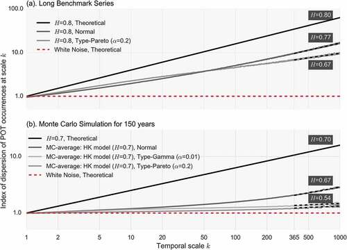
We test the dispersion index against samples of Gaussian and non-Gaussian time series exhibiting HK dynamics. Namely, we use (a) the two long benchmark series (N = 10⁶), the normal and the type-Pareto, both exhibiting H = 0.8; and (b) the ensemble of simulations of shorter length (equal to daily values for 150 years) for three different distributions, normal, type-gamma with shape parameter α = 0.01 and type-Pareto with α = 0.2, all exhibiting H = 0.7. For the second sample, we provide the average value estimated from the 10³ Monte Carlo simulations of the dispersion index at each scale. The results are shown in Fig. 5.

At first, it is worth noting that the onset scale, from which scaling arises, appears to be smaller for the long compared to the shorter time series. The related H parameters are estimated from Equation (3) for onset scale k₀ = 500, for both cases, in order to ensure a more robust estimate (yet fitted lines are extrapolated backwards to scale 365). It can be seen that the index yields satisfactory approximations of H only for the normal distribution and the long benchmark series (estimated H = 0.77, theoretical H = 0.8), whereas the results are biased downward for the non-Gaussian one (estimated H = 0.67, theoretical H = 0.8). In the case of the shorter record length, the bias severely increases as the index yields H parameters falsely denoting independence (average H = 0.54). There is also a considerable degree of ambiguity regarding the selection of the onset time, a task that requires visual examination and subjective judgement. For the above reasons, and due to the observed underestimation of persistence for common record lengths, we do not consider the index for the rest of the analysis. A more sophisticated use of the dispersion index, as well as bias correction methods, may be possible but remain out of the scope of this paper. For more information on a related index, the Allan factor, and its properties for testing independence the reader is referred to Serinaldi and Kilsby (2013).

3.5 A new probabilistic index to identify multi-scale clustering behaviour

The above review highlights the complexity involved in identifying clustering of extremes and the need to devise an informative and objective characterization able to reveal persistence even for non-Gaussian series, which are usually the ones of interest in geophysical studies. To address this, we formulate a straightforward and assumption-free representation of clustering by estimating the probability of occurrence of extreme events across multiple scales. The proposed probabilistic index is defined as follows.

We set a threshold to the original time series and select the data surpassing the threshold as extreme events, hence, forming the POT series, y_i. Accordingly, we form the series of counts of the POT events for each scale, z^(k), as explained in Section 3.1 (see also Fig. 2). We additionally, define the binary process ${\underset{\_}{r}}_q^{\left(k\right)}$ to denote the event of exceedence of the threshold at each time interval q of size k, q = 1, …, $⌊n/k⌋$:

(4) ${\underset{\_}{r}}_q^{\left(k\right)}:=\left\{\begin{array}{cc}1,& {\underset{\_}{z}}_q^{\left(k\right)}>0\\ 0,& {\underset{\_}{z}}_q^{\left(k\right)}=0\end{array}\right.$(4)

Then, the probability of exceedence of the threshold for timescale k is obtained as the frequency of exceedences estimated from all $⌊n/k⌋$ intervals:

(5) ${\bar{p}}^{\left(k\right)}=\frac{{\sum }_1^{⌊n/k⌋}{\underset{\_}{r}}_q^{\left(k\right)}}{⌊n/k⌋}$(5)

The latter is the exceedence probability (of the threshold) vs scale (EPvS) and its complement, $p^{\left(k\right)}=1-{\bar{p}}^{\left(k\right)}$ is the non-exceedence probability vs scale (NEPvS). Evidently, at scale k = 1 the EPvS is an estimate of the probability of the threshold value, ${\bar{p}}^{\left(1\right)}=F\left(u\right)$, and the NEPvs is $p^{\left(1\right)}=1-F\left(u\right)$. For example, in the previous applications, the threshold value was selected so that F(u) = 0.05. For a purely random process, the NEPvS is obtained as:

(6) $p^{\left(k\right)}=p^k$(6)

where p is the probability of non-exceedence at the basic scale k = 1 and equals 1 – F(u). Therefore, for white-noise processes, the probability of occurrence of extremes across scales is fully determined by the choice of the threshold (controlling its probability at the basic scale) and the scale. For HK processes though, a different behaviour is revealed, with the probabilities of non-exceedence of the threshold being larger than those obtained under independence. This property of HK is discussed and investigated extensively in the following Section 4.

To model the NEPvS, we revisit a probabilistic model proposed by Koutsoyiannis (2006) to describe the clustering behaviour of dry spells in rainfall time series. The model derives from an entropy-maximization framework and was originally proposed to describe the probability dry across different timescales. The latter, according to our definition, corresponds to a threshold taking the value of 0. Therefore, in a similar manner to the probability dry, we obtain the probability of non-exceedence of the threshold at scale k as:

(7) $p^{\left(k\right)}=p^{{\left[1+\left({\xi }^{-1/\eta }-1\right)\left(k-1\right)\right]}^{\eta }},p=1-F\left(u\right)$(7)

where u is the threshold parameter and η, ξ ϵ [0, 1]. For η = 1 and ξ = 0.5, Equation (7) describes the white-noise process. To allow backward extendibility to scale k = 0, the positivity of the base should be ensured and therefore the following inequality should hold: $\xi \ge 1/2^{\eta }$. We apply both the index and the proposed model to the synthetic series as well as to the rainfall data and assess their performance in characterizing clustering. We evaluate the index’s ability to reveal dependence by examining its performance for all the benchmark time series and we test its robustness by varying all the involved factors, i.e. sample size, marginal distribution’s properties and threshold value.

4 Results

4.1 Relating multi-scale clustering to LRD behaviour

We estimate the NEPvS index for the synthetic benchmark time series setting the threshold of extremes to 5%. The benchmark series have length 10⁶ and therefore for a 5% threshold we obtain 50 000 extreme values (POT events). We investigate the temporal scales 1 to 1000, since the index’s applicability to larger scales is to some extent also conditioned by the available sample size (this feature is discussed in Section 4.2).

Results from the NEPvS application are demonstrated on a double logarithmic plot of minus natural logarithm of the non-exceedence probability of the threshold vs the scale, which for most cases yields a straight line (Fig. 6). Some interesting insights can be derived. As persistence increases, the probability of no occurrences of extremes in a scale progressively increases (equivalently, its minus logarithm – shown in the plots – decreases), which is true for all the examined distribution types. As already mentioned, there is a maximum temporal scale until which the index is informative. The latter, which we will call the ‘max-discernible’ scale, is the scale for which the estimated (from the simulated series) non-exceedence probability equals zero as at least one extreme event is encountered in every one of the $n/k_{\mathrm{m}\mathrm{a}\mathrm{x}}$ intervals. In this case, the minus logarithm of the NEPvS tends to infinity and is not shown on the plots. For a given number of extremes and thus, sample size, the max-discernible scale depends on the H parameter; the larger the persistence, the more timescales are required in order to ‘encounter’ the extremes. This can be explained by considering that another manifestation of clustering of extremes is the existence of prolonged periods of time with no extreme occurrences.

It is worth noticing that the marginal properties are irrelevant for the NEPvS of the white-noise process. The latter is also proved in Fig. 6 as the lines of all the white-noise time series with different marginals are completely identical, for which there is a theoretical justification. Likewise, for H parameters no far from 0.5 the different non-Gaussian distributions (Fig. 6(a)) yield negligible differences on the NEPvS plots. However, notable differences appear for H > 0.7. Specifically, the non-Gaussian NEPvS plots evidently differ from the NEPvS of the normal distribution, especially for large H values, with the latter showing more apparent clustering behaviour.

Figure 6. Minus natural logarithm of non-exceedence probability vs scale (NEPvS) index on double logarithmic axes along with the fit of the proposed model (Equation 2) for (a) benchmark non-Gaussian time series (type-gamma and type-Pareto), and (b) benchmark normal time series, for a range of H parameters.

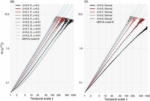
The NEPvS model (Equation 7) fits perfectly all the range of non-Gaussian distributions, with a slight exception for the normal time series at small scales (k < 50) and very large H parameter (H = 0.9).

4.2 NEPvS index sensitivity to sample size, threshold selection and distribution type

Having established that a representation in terms of the minus logarithm of probability vs timescale, like that of Fig. 6, reflects the presence of persistence for a range of distribution types, we aim to frame its statistical behaviour for different configurations of extreme value analysis. For this purpose, the statistical behaviour of this graph is investigated by means of Monte Carlo simulation starting from the white-noise case, which will serve as a benchmark model for identifying dependence from the rainfall data.

4.2.1 Sample size impact

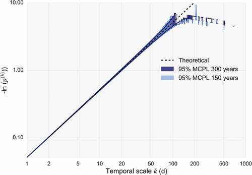
We generate two ensembles of 10³ white-noise time series with sample sizes 150 years (150 × 365 daily values) and 300 years, respectively, thus covering all the range of observed record lengths of our data set, and we produce the NEPvS plots for both lengths, shown in Fig. 7. As expected, the larger sample size produces narrower Monte Carlo Prediction Limits (MCPL), yet the difference is almost negligible. The fact that sample sizes of this order of magnitude yield only minimal differences in the MCPL gives confidence in attributing the differences between the models that are examined next to other factors instead. The essential change, however, between the two sample sizes is the propagation of the max-discernible scale to a larger timescale for the longer time series (Fig. 7). The latter is due to the fact that ‘extremes’ are distributed in longer time periods for the longer series, and therefore, the longer the series the more timescales may be inspected for clustering.

Figure 7. Minus natural logarithm of non-exceedence probability vs scale (NEPvS) index on double logarithmic axes for white-noise time series and two sample lengths: 150 × 365 and 300 × 365.

4.2.2 Threshold impact

The selection of the threshold is the most important choice when analysing records of maxima. It is generally acknowledged that choosing ‘high’ thresholds for the extremes results to observations that are located far in the right tail of the distribution, and therefore they are of interest, but simultaneously, increases uncertainty as the sampled observations are fewer. The exact opposite is true for lower thresholds. Therefore, one has to seek an optimal threshold compromising this trade-off.

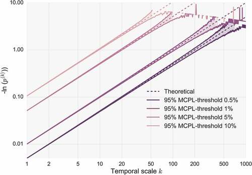
We first evaluate the choice of the threshold by examining four different thresholds associated with exceedence probabilities 0.5%, 1%, 5% and 10%, respectively, applied for the benchmark case of independence, as seen in Fig. 8. It is interesting to note that the main effect of the threshold for the iid case is the opportunity to apply the index to larger scales if the threshold is increased (smaller probability of exceedence). This is due to the fact that for the same record length, fewer extreme events are likely to be more separated in time and therefore, require longer timescales to be grouped.

Figure 8. Minus natural logarithm of non-exceedence probability vs scale (NEPvS) index on double logarithmic axes for white-noise time series (length 150 × 365) and variations of the sampling threshold of extremes.

We also inspect the impact of the threshold in relation to the H parameter of the parent process for three distribution types from the benchmark series, type-Pareto with a = 0.2, type-gamma with a = 0.01 and normal. In this case, we evaluate three different thresholds, 5%, 10% and 20%. Although the latter threshold would be considered ‘low’ for most extreme value analyses, here it is of interest, as by varying the threshold we aim to investigate the limits of identifiability of the HK behaviour, and not to focus on the exact shape of the distribution tail. To this aim, we fit the probabilistic model introduced in Equation (7) to each time series and evaluate the ability to reveal persistence through the identifiability of the fitted parameters, η and ξ. In Fig. 9, the impact of the threshold is striking within the same distribution with lower threshold values (e.g. 20%) increasing identifiability of the parameters more than 10%. Additionally, it can be seen that the η parameter is more sensitive to the normal distribution, while on the contrary the ξ parameter is sensitive to increasing skewness and kurtosis.

Figure 9. (a) Parameter η variation and (b) parameter ξ variation for increasing H parameter and different combinations of the sampling threshold and distribution type.

By performing the above experiments, we have demonstrated the twofold effect of the threshold: ‘lower’ thresholds (higher probability of exceedence) enable better identifiability of persistence, yet they limit application of the index to less scales, and vice versa.

4.2.3 Distribution type

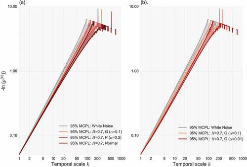
At this stage, for the same threshold (5%), sample size (150 years) and H (0.7) parameter, we estimate the NEPvS index for the shorter benchmark series characterized by different marginal properties, and thus distribution tails, so as to focus solely on the impact of skewness and kurtosis on the index. The results are plotted in Fig. 10. Two important conclusions can be drawn: (a) clustering of extremes and its identifiability is, in this case too, greater for the normal distribution (Fig. 10(a)), and (b) for a specified non-Gaussian distribution, clustering is greater and also more visible for increasing skewness and kurtosis (Fig. 10(b)). The latter is a significant advance as the reviewed tools in sections 3.3 and 3.4 showed very high downward bias for increasing higher order moments of the non-Gaussian distributions and practically no difference among them for the record lengths available (150 years). We also provide the plots of the fitting of η and ξ parameters computed for the long benchmark series with H parameters in the range [0.5 0.99], as well as their comparison, in the Appendix (Figures A1–A3), where all three plots confirm the above observations.

Figure 10. Minus natural logarithm of non-exceedence probability vs scale (NEPvS) index on double logarithmic axes along with 95% MCPL for (a) H = 0.7 with type-gamma (α = 0.1) and type-Pareto (α = 0.2) and white noise, and (b) H = 0.7 for two type-gamma distributions with α = 0.1 and α = 0.01.

4.3 Clustering in real-world rainfall extremes I: identifying clustering mechanisms in the parent process

Rainfall is a complex geophysical process for the stochastic modelling of which it is necessary to take into account its mixed-type marginal distribution (due to intermittency), the presence of cyclo-stationarity (seasonality and also diurnal cycle for sub-daily scales), as well as its scale dependence structure (Markonis and Koutsoyiannis 2016). It is expected that all these mechanisms affect the clustering process of extremes.

In the following, we investigate their impact separately, although we note that the interplay among them may not necessarily allow the robust disentanglement of their effects at the different scales.

4.3.1 Influence of probability dry

The most distinctive feature of the rainfall process is its highly intermittent nature at fine temporal scales (Koutsoyiannis 2006). To statistically account for intermittency, the marginal distribution is formed as a mixed (discrete-continuous) type one, having a probability mass function concentrated at 0 and a probability distribution function to describe the nonzero values. Therefore, if p_d is the probability of no-rain, termed ‘probability dry’, then the cumulative distribution function for the whole rainfall record $F_{\underset{\_}{x}}\left(x\right)$ can be defined in terms of the conditional distribution of wet days $F_{\underset{\_}{x}\left|\underset{\_}{x}\right.⟩0}\left(x\right)$ as:

(8) $F_{\underset{\_}{x}}\left(x\right)=\left(1-p_{\text{d}}\right)F_{(\underset{\_}{x}|\underset{\_}{x}>0)}(x)+p_{\text{d}},x\ge 0$(8)

Since the threshold of extremes u is obtained as the quantile with a chosen probability of exceedence, it is evident that in the case of mixed-type processes, as in daily rainfall, the same threshold value will have a different probability of exceedence for the whole process and for the wet process (the nonzero rainfall). By simple probabilistic statements, it follows that the two exceedence probabilities of the threshold u for the compound and the wet process, p_c(u) and p_w(u), respectively, are related as:

(9) $p_{\mathrm{w}}\left(u\right)=\frac{p_{\mathrm{c}}\left(u\right)}{1-p_{\mathrm{d}}}$(9)

where p_d = 1 – p_c(0) is the probability dry. Therefore, the exceedence probability for the same threshold is higher for the wet series, which means that depending on the probability dry, the values surpassing the same threshold may not necessarily belong to the right tail of the wet series as ‘extremes’. For instance, a threshold u with associated exceedence probability 5% for the whole rainfall record with probability dry equal to 80% yields exceedence probability 25% for the wet series, and therefore the resulting series of POT events would also include lower rainfall values. While this is not a limitation of the methodology, it should be properly accounted for in order to (a) ensure that the resulting extremes are indeed towards the right end of the wet series tail and (b) make meaningful comparisons among stations with different values of the probability dry. For this reason, we compute p_d for all stations in order to make sure that the resulting extremes are surpassing relevant thresholds. As previously shown, the latter is important since the threshold is the key control on the results.

4.3.2 Influence of seasonality

Seasonality may be in cases an important attribute of extreme rainfall impacting the central tendency of rainfall maxima belonging to different seasons and inducing temporal clustering in the series of extremes (Iliopoulou et al. 2018). Since our aim is to focus on the impact of HK dynamics on clustering of extremes, we apply deseasonalization schemes to the original series in order to smooth out the seasonal components and reduce associated clustering. By doing so, we may perform Monte Carlo simulations with one marginal distribution per station for the validation of the chosen models. We note that a perfect separation of the impact of seasonality from HK dynamics may not always be possible, as in stations exhibiting strong seasonality we anticipate interplay between the two.

We consider two different methods for removing seasonality. The first one, termed M1, is a simple standardization scheme performed on a monthly basis. The daily values x_i belonging to each month, m (m = 1, …, 12) are transformed by subtracting the mean and dividing by the standard deviation of all daily values belonging to the same month, as follows: $y_i=(x_i-{\mu }_m)/{\sigma }_m,i\in m$. This method effectively removes seasonality from the first two moments of the data. In order to deal with higher order moments, we apply a second deseasonalization scheme denoted M2, which is based on the normal quantile transformation (NQT) also applied on a monthly basis. 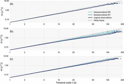The daily series for each month m are transformed to standard Gaussian quantiles through the inverse function of the standard Gaussian cumulative distribution, $y_i={G_m}^{-1}\left(F\left(x\right)\right)$, with their cumulative probability F(x) estimated via their Weibull plotting position. Consequently, after the transformation, all daily values of each month follow the standard normal distribution. We found that the two schemes show minimal differences in the behaviour of the index, with the most apparent ones belonging to the stations of Athens (Fig. 11(b)), Palermo and Lisbon.

In Fig. 11, we plot three characteristic cases of the NEPvS behaviours found in the data: (a) in a typical station with minimal to no seasonality (Oxford), where extremes are not affected by deseasonalization schemes (Fig. 11(a)); (b) in a station with prominent seasonality (Athens, Fig. 11(b)), where a stronger deseasonalization scheme (M2) maybe required; and (c) in an intermediate case (Helsinki, Fig. 11(c)), where the seasonal component in extremes is effectively dealt by with the simpler scheme (M1). The majority of the stations (40) belong to the third category, while for 17 stations accounting for seasonality yields minimal to no difference. These findings are consistent in general with the analysis of Iliopoulou et al. (2018) on the presence of seasonality in extreme rainfall.

Figure 11. Minus natural logarithm of non-exceedence probability vs scale (NEPvS) index on double logarithmic axes for white-noise time series and seasonal and deseasonalized series by methods 1 (M1) and 2 (M2) for the stations of (a) Oxford, (b) Athens and (c) Helsinki.

4.3.3 Rainfall scaling regimes

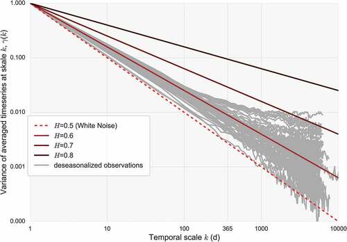
In order to highlight the motivation behind selecting the daily rainfall as a case study for the method and establish the ‘target’ persistence structure that we aim to reveal, we estimate the persistent properties of the previously deseasonalized daily rainfall series. To this aim, we compute the H parameter through the climacogram as introduced in Section 3.3 All the empirical climacograms are plotted in Fig. 12. The estimated average persistence (Table 2) is close, but even larger than the global estimate (H ≈ 0.6) of Iliopoulou et al. (2016) concerning annual rainfall. Remarkably, in many stations we observe a change of the scaling regime, namely an intensification of persistence, at scales above yearly. A similar result was observed in the work of Markonis and Koutsoyiannis (2016) for rainfall records at the over-decadal scale. This behaviour is also evident in Table 2, which reports the estimated H parameters for the daily and above-yearly scales.

Table 2. Summary statistics (first and third quantiles, Q1 and Q3, mean and standard deviation, SD) of the properties of the rainfall dataset. Mean, variance, skewness and kurtosis are estimated for the wet record.

Statistic	Mean	Variance	Skewness	Kurtosis	Prob. dry	Hdaily	Hannual		Years	Missing %
Q1	3.68	24.85	2.9	17.28	0.47	0.56		0.55	153	0.75
Mean	4.98	64.85	3.39	24.03	0.55	0.63		0.67	169.25	2.62
Q3	5.91	64.64	3.54	25.85	0.61	0.7		0.77	173	1.31
SD	2.27	94.15	0.72	10.94	0.11	0.09		0.13	24.66	5.11

Figure 12. Empirical climacograms of the 60 daily rainfall series used in the analysis along with theoretical lines for H = 0.5, 0.6, 0.7, 0.8.

4.4 Clustering in real-world rainfall extremes II: HK dynamics?

4.4.1 Analysis of daily rainfall extremes in the Netherlands

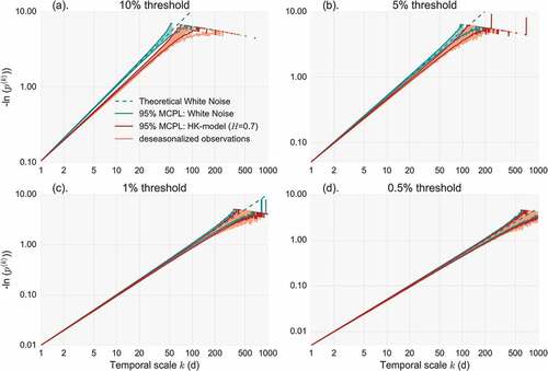
It should be evident by now that the clustering dynamics of extremes depend not only on the persistent properties of the parent process but on its higher-order moments as well. The identifiability of clustering also varies depending on the choice of the threshold, which may need to be modified for mixed type processes, as discussed before. In our case, this means that depending on the probability dry of each station, the chosen threshold will correspond to a different one for the ‘wet’ record of each station. Therefore, a blind comparison of different stations with the obtained MCPL for a given threshold could be uninformative depending on the variability of probability dry in the sample of the stations. In order to apply the methodology effectively in as many stations as possible we assume a climatically homogenous regions in which the rainfall time series can be regarded as realizations of a single process. For this purpose, we select the region of the Netherlands, in which 28 of the 60 stations are located, and preliminary analysis showed small variability of the summary statistics. We estimate the average values of the first four moments of the deseasonalized records for all 28 stations and we also estimate the H parameter resulting from the analysis of the daily values. We form an ensemble of 10³ Monte Carlo simulations for the average number of years of the sample (160 years), with an HK-model preserving the first four moments and, subsequently, compare its clustering behaviour with the one observed from the sample of the stations. We also repeat the Monte Carlo simulation for a white-noise process. We present both cases in Fig. 13. It is evident that the assumed model is consistent with the majority of the observed records, with only a few stations located in the southwest of the Netherlands exhibiting even stronger clustering outside of the 95% region of the assumed HK model. As expected, as the threshold increases evidence of persistence is progressively ‘lost’ and the probabilistic behaviour of POT occurrences approaches a random one.

Figure 13. Minus natural logarithm of non-exceedence probability vs scale (NEPvS) index on double logarithmic axes for deseasonalized series for the 28 rainfall records in The Netherlands along with 95% MCPL of the fitted model with H = 0.7, for four different thresholds: (a) 10%, (b) 5%, (c) 1% and (d) 0.5%.

4.4.2 Stykkisholmur case study

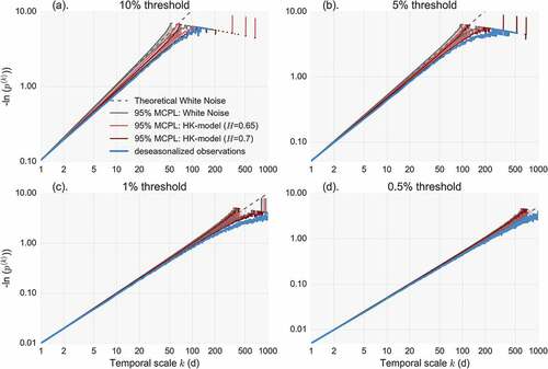
As a second case study, we select a single station located in Stykkisholmur, Iceland, which is the station with the most peculiar behaviour among all those we analysed. We repeat the Monte Carlo analysis for both a white-noise process and a HK process preserving the first four moments and the H (= 0.65) parameter of the record. The results are shown in Fig. 14. It is interesting to note that clustering in this case appears stronger than predicted by the HK model. The Monte Carlo experiment is repeated for H = 0.7 to explore the possible impact of estimation uncertainty due to the standard deviation bias in finite sample sizes (Koutsoyiannis and Montanari 2007). In this case, the MCPL approach the observed data for the lower threshold, yet the impact is lower for the higher threshold. A similar behaviour was found in the station of Uppsala, Sweden. We hypothesize that this ‘discrepancy’ between the persistence found in the parent process and the stronger one implied by the extremes might be explained by the impact of large-scale atmospheric circulation patterns (such as the North Atlantic Oscillation, NAO) on rainfall extremes, which might need even longer record lengths in order to be effectively summarized by the second-order characterization provided by the H parameter.

Figure 14. Minus natural logarithm of non-exceedence probability vs scale (NEPvS) index on double logarithmic axes for the deseasonalized series of Stykkisholmur, Iceland, along with 95% MCPL of the fitted models with H = 0.65 and H = 0.7, for four different thresholds: (a) 10%, (b) 5%, (c) 1% and (d) 0.5%.

4.4.3 Modeling the clustering behaviour

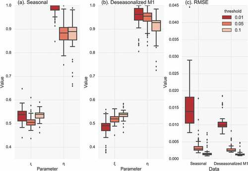
We apply the NEPvS model to both seasonal and deseasonalized time series of the rainfall data of all 60 stations in order to assess its applicability in all cases. We employ the deseasonalized scheme M1. In Fig. 15 we plot the boxplots of the estimated parameters η and ξ as well as the RMSE for the seasonal and the deseasonalized series for three different thresholds, 1%, 5% and 10%. From the fitted parameters, it is reaffirmed by this analysis as well that, as the threshold decreases, the estimates of the parameters deviate from the ones obtained for the iid case (ξ = 0.5 and η = 1). From the RMSE (Fig. 15(c)), it can be seen that the proposed model describes very well the deseasonalized data and fairly well the original observations, and in both cases the modelling efficiency improves for lower thresholds. Seasonality is associated with increased temporal clustering at the intermediate scales (approx. 20–150 days), which manifests with a curvature in the NEPvS plots that the model captures less efficiently compared to the deseasonalized case, typically producing a straight line plot. Also, it is evident that the results concerning the threshold are not as robust for this case, since the impact of the threshold on seasonal clustering may vary depending on the specific seasonal regime. For instance, it is expected that for stations with prominent seasonality, high thresholds will show increased clustering only in the wettest season, whereas lower threshold will enable inspection of clustering in more seasons. However, depending on the characteristics of the seasonal regime and the intensity of the specific seasons, the temporal mixture of extremes from the different seasons differs from case to case and, thus, it is not straightforward to discern the impact of seasonality from a bulk fitting to all cases. On the other hand, for the deseasonalized cases it is clear that ‘dependence’ emerges as the threshold lowers.

Figure 15. Boxplots of (a) parameter η, (b) parameter ξ and (c) RMSE from the fitting of the model to the seasonal and deseasonalized series by M1 for three different thresholds (1%, 5% and 10%).

5 Discussion

Clustering of extreme events is related to the presence of persistence, or HK dynamics, in natural processes. Here we approached this relationship with a twofold intention; first to ‘retrieve’ persistence from records of maxima and, second, to characterize it by probabilistic means. To this aim, we have introduced the NEPvS index, for which we also propose a model. The index examines the probabilistic behaviour of POT occurrences across multiple scales, and proved successful in revealing persistence from extremes from various non-Gaussian time series, for which well-known tools performed poorly.

It seems, though, to be difficult to establish general analytical relationships linking the NEPvS behaviour to the H parameter of the parent process, which is true without even considering the uncertainty involved in estimating H from small record lengths in the first place. As the H parameter is a second-order characterization of a process, generation schemes reproducing H behaviour but coupled with different marginal distributions (having different high-order moments), will yield different behaviours of extremes. For instance, clustering of extremes and its identifiability appears to be much more prominent in Gaussian processes. The task, therefore, of linking clustering of extremes to the H parameter, without also accounting for the specific high order moments of the time series, seems infeasible. We showed, though, that the threshold is a key determinant in this respect, as lowering the threshold, i.e. moving towards the central tendency of the data, enables better identification of persistence. In contrast, as the threshold increases, evidence of persistence is progressively lost and the behaviour of extremes may falsely suggest independence of the parent process.

Application of the NEPvS index to daily rainfall data showed that there may exist significant departures from independence, particularly for lower thresholds, which are dependent on the location and specific climatic region. In general, the behaviour of rainfall extremes in multiple case studies (28 stations in the Netherlands and one in Iceland) was found by means of extensive Monte Carlo simulations, to be consistent with HK dynamics characterized by moderate H parameters (in the range 0.6–0.7). The NEPvS model showed a very good fit to the probabilistic behaviour of exceedences for the seasonal and deseasonalized observations across multiple scales for all 60 stations. As a similar version of the model has been previously proposed to describe the probability dry across multiple scales (Koutsoyiannis 2006), this result suggests that there exists a probabilistic law which effectively describes the multi-level exceedences of rainfall thresholds across scales, from zero-crossings (wet days) to high-level crossings, as the ones examined here.

From a theoretical point of view, these findings suggest that it is important to study change and clustering in a consistent stochastic framework examining the whole process behaviour, in order to better understand the process dynamics and avoid retaining ‘preconceived’ assumptions, such as iid, which may be inconsistent with the physical reality. For instance, various trend tests assume iid for the examined process, while modified tests accounting for persistence (Hamed 2008), also do not consider its interplay with the higher order moments. Therefore, it is likely that they fail to account for extremes from complex processes, leaving aside issues regarding problematic applications due to misinterpretation of stationarity (Montanari and Koutsoyiannis 2014, Koutsoyiannis and Montanari 2015). Overdispersion in POT rainfall events has been also studied lately and attributed to a mixture of Poisson models, representing different climate regimes (Tye et al. 2019) as well as seasonality mechanisms (Serinaldi and Kilsby 2013). Although, we have found as well that in some cases seasonality accounts for most of the observed clustering in the rainfall extremes, by performing multiple MC experiments focusing on the deseanonalized extremes, we have revealed consistency with HK dynamics. We note though that as the H parameter for rainfall revolves around the value of 0.6 and rainfall is a heavily skewed process, it is expected that identifiability of persistence from extremes will be limited, except if one lowers the threshold. Nevertheless, this highlights an alternative scientific hypothesis to be considered in ‘attribution’ studies, which is the emergence of clustering and overdispersion of extremes from persistence in the parent process.

From a practical point of view, the presence of persistence in the parent process affects estimation of extreme values and, therefore, various design outcomes, in multiple ways. Although the theoretical definition of return period is still valid under the presence of persistence (Koutsoyiannis 2008, Volpi et al. 2015), the statistical estimates of distribution quantiles for a specified return period are severely impacted. Other important implications concern flood risk underestimation under the presence of persistence (Serinaldi and Kilsby 2016), as well as underestimation of IDF (intensity–duration–frequency) curves when the temporal dependence is disregarded (Roy et al. 2019). Therefore, although persistence of the parent process is less evident in the series of its extremes, and it is highly unlikely that it can be fully retrieved except for very low thresholds, its impact cannot be disregarded when studying extremes, even if the latter appear independent. Yet theoretical arguments exist concerning the validity of well-known theorems under relaxed assumptions of iid, for instance fundamental EVT results (limiting distributions etc.) which hold true under weak presence of persistence (Leadbetter 1983). However, for scientific applications, which involve estimation from data of finite, and typically small record lengths, the presence of persistence in the process induces uncertainty in the estimation, as the actual information content of the data is lower than that for iid conditions (Koutsoyiannis and Montanari 2007), and this uncertainty inevitably propagates into the extreme value estimates.

The existence of clustering also increases the arguments towards the use of the POT method for sampling of extremes, instead of block maxima approaches which tend to hide dependence, as also evident in Fig. 2. As the threshold plays a vital role, using POT approaches with more than one event per year, on average, which is the common practice, is also equally important. Empirical declustering approaches (Lang et al. 1999) may also be non-effective if they do not take into account each process characteristics. In this regard, we argue that instead of seeking to resort to independence, often at the cost of reducing the available information (e.g. by discounting ‘dependent’ data), accounting for dependence is a more viable and consistent way forward. In fact, the use of the whole set of observations has been recently advocated (Volpi et al. 2019), while the emergence of new types of high-order moments (Koutsoyiannis 2019) that exploit the whole set of observations provides an improved stochastic framework for applying this principle.

6 Conclusions

This research deals with the question of identifying the links between persistence in the parent process and clustering of extremes, with the specific aim to ‘rediscover’ the usually ‘lost’ persistence when one examines records of maxima. This is achieved by devising a probabilistic characterization of clustering of extremes. The main findings are summarized below:

1. There is significant influence from both the second-order properties and the high-order moments of the parent process on the generated extremes and, therefore, characterizations of clustering of extremes need to account for both.

2. Identifiability of persistence from records of maxima is, in general, limited and weakens as the threshold for extremes increases.

3. The estimates of the Hurst parameter from the climacogram analysis and from the dispersion index are found to be severely biased downward when derived from extremes originating from non-Gaussian processes.

4. A new probabilistic index is proposed to represent clustering based on the probability of non-exceedence of a given threshold across scales, called the NEPvS (non-exceedence probability vs scale) index.

5. The NEPvS exhibits scaling behaviour which is described by a proposed model accurately simulating the probability of exceedence of a threshold at multiple temporal scales.

6. The index is transparent and can be directly used for statistical testing of departures from independence. Case-specific Monte Carlo simulations are needed to validate more complicated models coupling persistence with different marginal properties.

7. The POT approach applied with ‘low’ thresholds is a robust and informative way to reveal the clustering dynamics of extremes, in contrast to the block maxima method which hinders identifiability of persistence.

8. Deseasonalized daily rainfall POT events may show prominent departures from independence especially at lower thresholds, which may become important depending on the climatic region. Extensive station-specific Monte Carlo experiments showed consistency of clustering of extremes for various examined thresholds with assumed HK models fitted based on the properties of the parent process.

Further research is required in order to obtain analytical mathematic results for extremes arising from persistent processes, with the aim of constructing estimators for any distribution type and dependence structure without the need for Monte Carlo validations. However, the latter is doubtful as a task, since extremes over scales are controlled by higher-order moments, which are also difficult to estimate correctly from data (Lombardo et al. 2014). Recently proposed moment types with unbiased estimators across all orders that can also model joint properties of processes could provide a way to circumvent this (Koutsoyiannis 2019).

We conclude that extremes tend to ‘hide’ the persistence of the parent process, often falsely signalling independence. However, regardless of the strength of the evidence, the impact of persistence in the parent process on the estimation of extreme values is nonetheless present. In this respect, more research should focus on the stochastic properties of extremes from natural processes, where dependence mechanisms manifest themselves across various temporal scales and challenge common assumptions and practices.

Acknowledgements

We greatly thank the Radcliffe Meteorological Station, the Icelandic Meteorological Office (Trausti Jónsson), the Czech Hydrometeorological Institute, the Finnish Meteorological Institute, the National Observatory of Athens, the Department of Earth Sciences of the Uppsala University and the Regional Hydrologic Service of the Tuscany Region ([email protected]) for providing the required data for each region respectively. We are also grateful to Professor Ricardo Machado Trigo (University of Lisbon) for providing the Lisbon time series, to Professor Marco Marani (University of Padua) for providing the Padua time series and to Professor Joo-Heon Lee (Joongbu University) for providing the Seoul time series. All the above data were freely provided after contacting the acknowledged sources. The remaining time series are publicly available by the data providers in the ECA&D project (http://www.ecad.eu), and in the GHCN-Daily database (https://data.noaa.gov/dataset/global-historical-climatology-network-daily-ghcn-daily-version-3). The analyses were performed in the Python 2.6 (Python Software Foundation. Python Language Reference, version 2.7, available at http://www.python.org) using the contributed packages pandas, scipy and seaborn. The codes used for the generation of the synthetic SMA series (Dimitriadis and Koutsoyiannis, 2018) are available at: https://www.itia.ntua.gr/en/docinfo/1656/. We are grateful to the Associate Editor Elena Volpi and the anonymous reviewer for the encouraging and constructive comments.

Disclosure statement

No potential conflict of interest was reported by the authors.

Appendix I

Figure A1. Plots of η and ξ parameters vs the H parameter and polynomial fitting for the distributions: (a) type-Pareto with α = 0.1, (b) type-Pareto with α = 0.2, (c) type-gamma with α = 0.1 and (d) type-gamma with α = 0.01.

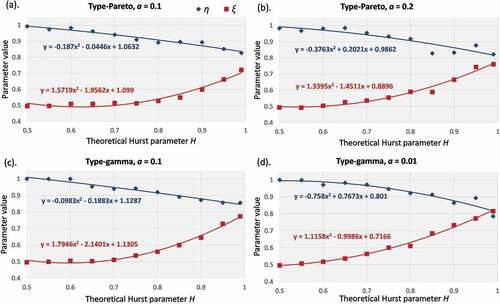
Figure A2. Plots of η and ξ parameters vs the H parameter and polynomial fitting for the normal distribution.

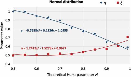
Figure A3. Plots of η and ξ parameters vs the H parameter for the distributions type-Pareto, with α = 0.1 and α = 0.2, type-gamma with α = 0.1 and α = 0.01 and normal.

References

- Barunik, J. and Kristoufek, L., 2010. On hurst exponent estimation under heavy-tailed distributions. Physica A: Statistical Mechanics and Its Applications, 389, 3844–3855. doi:10.1016/j.physa.2010.05.025
- Coles, S., et al., 2001. An introduction to statistical modeling of extreme values. Berlin, Germany: Springer.
- Dimitriadis, P., 2017. Hurst-Kolmogorov dynamics in hydrometeorological processes and in the microscale of turbulence. Thesis. National Technical University of Athens, Athens, Greece.
- Dimitriadis, P. and Koutsoyiannis, D., 2015. Climacogram versus autocovariance and power spectrum in stochastic modelling for Markovian and Hurst–Kolmogorov processes. Stochastic Environmental Research and Risk Assessment, 29, 1649–1669. doi:10.1007/s00477-015-1023-7
- Dimitriadis, P. and Koutsoyiannis, D., 2018. Stochastic synthesis approximating any process dependence and distribution. Stochastic Environmental Research and Risk Assessment, 32, 1493–1515. doi:10.1007/s00477-018-1540-2
- Eichner, J.F., et al., 2011. The statistics of return intervals, maxima, and centennial events under the influence of long-term correlations. In J. Kropp, S.H. Joachim, eds. In extremis. Berlin, Germany: Springer, 2–43.
- Ferro, C.A. and Segers, J., 2003. Inference for clusters of extreme values. Journal of the Royal Statistical Society: Series B (statistical Methodology), 65, 545–556. doi:10.1111/1467-9868.00401
- Hamed, K.H., 2008. Trend detection in hydrologic data: the Mann-Kendall trend test under the scaling hypothesis. Journal of Hydrology, 349, 350–363. doi:10.1016/j.jhydrol.2007.11.009
- Hurst, H.E., 1951. Long-term storage capacity of reservoirs. Transactions of the American Society of Civil Engineers, 116, 770–808.
- Iliopoulou, T., et al., 2016. Revisiting long-range dependence in annual precipitation. Journal of Hydrology, 556 (January 2018), 891–900. doi:10.1016/j.jhydrol.2016.04.015
- Iliopoulou, T., Koutsoyiannis, D., and Montanari, A., 2018. Characterizing and modeling seasonality in extreme rainfall. Water Resources Research, 54, 6242–6258. doi:10.1029/2018WR023360
- Klein Tank, A.M.G., et al., 2002. Daily dataset of 20th-century surface air temperature and precipitation series for the European climate assessment. International Journal of Climatology, 22, 1441–1453. doi:10.1002/joc.773
- Kottegoda, N.T. and Rosso, R., 2008. Applied statistics for civil and environmental engineers. Malden, MA: Blackwell.
- Koutsoyiannis, D., 2003. Climate change, the Hurst phenomenon, and hydrological statistics. Hydrological Sciences Journal, 48, 3–24. doi:10.1623/hysj.48.1.3.43481
- Koutsoyiannis, D., 2006. An entropic-stochastic representation of rainfall intermittency: the origin of clustering and persistence. Water Resources Research, 42.
- Koutsoyiannis, D., 2008. Probability and statistics for geophysical processes. National Technical University of Athens, Athens, Greece.
- Koutsoyiannis, D., 2010. HESS opinions a random walk on water”. Hydrology and Earth System Sciences, 14, 585–601. doi:10.5194/hess-14-585-2010
- Koutsoyiannis, D., 2016. Generic and parsimonious stochastic modelling for hydrology and beyond. Hydrological Sciences Journal, 61 (2), 225–244. doi:10.1080/02626667.2015.1016950
- Koutsoyiannis, D., 2019. Knowable moments for high-order stochastic characterization and modelling of hydrological processes. Hydrological Sciences Journal, 64 (1), 19–33. doi:10.1080/02626667.2018.1556794
- Koutsoyiannis, D. and Montanari, A., 2007. Statistical analysis of hydroclimatic time series: uncertainty and insights. Water Resources Research, 43.
- Koutsoyiannis, D. and Montanari, A., 2015. Negligent killing of scientific concepts: the stationarity case. Hydrological Sciences Journal, 60 (7–8), 1174–1183. doi:10.1080/02626667.2014.959959
- Lang, M., Ouarda, T., and Bobée, B., 1999. Towards operational guidelines for over-threshold modeling. Journal of Hydrology, 225, 103–117. doi:10.1016/S0022-1694(99)00167-5
- Leadbetter, M.R., 1983. Extremes and local dependence in stationary sequences. Probability Theory and Related Fields, 65, 291–306.
- Lombardo, F., et al., 2014. Just two moments! A cautionary note against use of high-order moments in multifractal models in hydrology. Hydrology and Earth System Sciences, 18, 243–255. doi:10.5194/hess-18-243-2014
- Marani, M. and Zanetti, S., 2015. Long-term oscillations in rainfall extremes in a 268 year daily time series. Water Resources Research, 51, 639–647. doi:10.1002/2014WR015885
- Markonis, Y. and Koutsoyiannis, D., 2016. Scale-dependence of persistence in precipitation records. Nature Climate Change, 6, 399–401. doi:10.1038/nclimate2894
- Menne, M.J., et al., 2012. An overview of the global historical climatology network-daily database. Journal of Atmospheric and Oceanic Technology, 29, 897–910. doi:10.1175/JTECH-D-11-00103.1
- Merz, B., Nguyen, V.D., and Vorogushyn, S., 2016. Temporal clustering of floods in Germany: do flood-rich and flood-poor periods exist? Journal of Hydrology, 541, 824–838. doi:10.1016/j.jhydrol.2016.07.041
- Montanari, A., 2003. Long-range dependence in hydrology. Theory and Applications of Long-range Dependence, 461–472.
- Montanari, A. and Koutsoyiannis, D., 2014. Modeling and mitigating natural hazards: stationarity is immortal! Water Resources Research, 50, 9748–9756. doi:10.1002/2014WR016092
- Ntegeka, V. and Willems, P., 2008. Trends and multidecadal oscillations in rainfall extremes, based on a more than 100-year time series of 10 min rainfall intensities at Uccle, Belgium. Water Resources Research, 44. doi:10.1029/2007WR006471
- O’Connell, P.E., et al., 2016. The scientific legacy of Harold Edwin Hurst (1880–1978). Hydrological Sciences Journal Special Issue: Facets of Uncertainty, 61 (9), 1571–1590. doi:10.1080/02626667.2015.1125998
- Papoulis, A., 1991. Probability, random variables, and stochastic processes. 3rd. New York, NY: McGraw-Hill.
- Roy, T., et al., 2019. A probabilistic intensity-duration-frequency framework considering temporal dependence (in preparation).
- Serinaldi, F., 2013. On the relationship between the index of dispersion and Allan factor and their power for testing the poisson assumption. Stochastic Environmental Research and Risk Assessment, 27, 1773–1782. doi:10.1007/s00477-013-0699-9
- Serinaldi, F. and Kilsby, C.G., 2013. On the sampling distribution of Allan factor estimator for a homogeneous poisson process and its use to test inhomogeneities at multiple scales. Physica A: Statistical Mechanics and Its Applications, 392, 1080–1089. doi:10.1016/j.physa.2012.11.015
- Serinaldi, F. and Kilsby, C.G., 2016. Understanding persistence to avoid underestimation of collective flood risk. Water, 8, 152. doi:10.3390/w8040152
- Serinaldi, F. and Kilsby, C.G., 2018. Unsurprising surprises: the frequency of record-breaking and overthreshold hydrological extremes under spatial and temporal dependence. Water Resources Research, 54, 6460–6487. doi:10.1029/2018WR023055
- Tegos, A., et al., 2017. An R function for the estimation of trend significance under the scaling hypothesis-application in PET parametric annual time series. Open Water Journal, 4, 6.
- Telesca, L., et al., 2002. On the methods to identify clustering properties in sequences of seismic time-occurrences. Journal of Seismology, 6, 125–134. doi:10.1023/A:1014275509447
- Thurner, S., et al., 1997. Analysis, synthesis, and estimation of fractal-rate stochastic point processes. Fractals, 5, 565–595. doi:10.1142/S0218348X97000462
- Tye, M.R., Katz, R.W., and Rajagopalan, B., 2019. Climate change or climate regimes? Examining multi-annual variations in the frequency of precipitation extremes over the argentine pampas. Climate Dynamics, 53 (1–2), 245–260. doi:10.1007/s00382-018-4581-9
- Tyralis, H., et al., 2018. On the long-range dependence properties of annual precipitation using a global network of instrumental measurements. Advances in Water Resources, 111, 301–318. doi:10.1016/j.advwatres.2017.11.010
- Tyralis, H. and Koutsoyiannis, D., 2011. Simultaneous estimation of the parameters of the Hurst–Kolmogorov stochastic process. Stochastic Environmental Research and Risk Assessment, 25, 21–33. doi:10.1007/s00477-010-0408-x
- Vitolo, R., et al., 2009. Serial clustering of intense European storms. Meteorologische Zeitschrift, 18, 411–424. doi:10.1127/0941-2948/2009/0393
- Volpi, E., et al., 2015. One hundred years of return period: strengths and limitations. Water Resources Research, 51, 8570–8585. doi:10.1002/wrcr.v51.10
- Volpi, E., et al., 2019. Save hydrological observations! Return period estimation without data decimation. Journal of Hydrology, 571, 782–792. doi:10.1016/j.jhydrol.2019.02.017.
- Willems, P., 2013. Adjustment of extreme rainfall statistics accounting for multidecadal climate oscillations. Journal of Hydrology, 490, 126–133.