Modelling of infiltration using artificial intelligence techniques in semi-arid Iran

ABSTRACT

Infiltration plays a fundamental role in streamflow, groundwater recharge, subsurface flow, and surface and subsurface water quality and quantity. In this study, adaptive neuro-fuzzy inference system (ANFIS), support vector machine (SVM) and random forest (RF) models were used to determine cumulative infiltration and infiltration rate in arid areas in Iran. The input data were sand, clay, silt, density of soil and soil moisture, while the output data were cumulative infiltration and infiltration rate, the latter measured using a double-ring infiltrometer at 16 locations. The results show that SVM with radial basis kernel function better estimated cumulative infiltration (RMSE = 0.2791 cm) compared to the other models. Also, SVM with M4 radial basis kernel function better estimated the infiltration rate (RMSE = 0.0633 cm/h) than the ANFIS and RF models. Thus, SVM was found to be the most suitable model for modelling infiltration in the study area.

KEYWORDS:

• infiltration
• adaptive neuro fuzzy inference system
• random forest
• support vector machine

Editor S. Archfield Associate editor F.-J. Chang

1 Introduction

Infiltration is fundamental for irrigated agriculture and for streamflow, groundwater recharge, subsurface flow, and surface and subsurface water quality and quantity, Precipitation is separated into surface and subsurface flows through infiltration. The action of infiltration through soil is influenced by several factors, such as antecedent soil moisture, soil texture and type, soil density, hydraulic conductivity and precipitation, as welll as hydrological features (Angelaki et al. 2018, Singh et al. 2018b). Numerous models have been developed for estimating infiltration by various researchers, such as Green and Ampt (1911), Kostiakov (1932), Horton (1941), Holtan (1961) Philip (1957a, 1957b), the Soil Conservation Service (SCS) (1972), Parlange (1971a, 1971b, 1972a, 1972b, 1975, 1982, 1985), Singh and Yu (1990), Corradini et al. (1994), as well as Sihag et al. (2017a). Most of these models are point or local and assume that soil is homogeneous with constant moisture content and constant hydraulic conductivity. Only a few models have been effectively implemented in the field or at large spatial scales. Some of the models have also been compared (see Angelaki et al. 2013).

The physical and hydraulic characteristics of soil often vary at different locations in the same watershed, and the temporal and spatial inconsistency of soil properties is a major obstacle in the estimation of infiltration at the basin scale (Babaei et al. 2018). The spatial variability of infiltration rate – due to both crop type and agricultural practices – makes irrigation water management difficult.

Soils are not often homogeneous. In hydrological forecasting, effective precipitation is schematized using a two-layered vertical soil profile (Taha et al. 1997). Upscaling of local infiltration modelling to the field scale is needed, which is difficult because of the spatial variability of soil and its hydraulic properties (Loague and Gander 1990). Local physical infiltration models are based on the law of mass conservation and Darcy’s law; empirical models rely on field and laboratory measurements, and semi-empirical models are based on simple hypotheses on the relationship between infiltration rate and cumulative infiltration. The latter infiltration models have been developed for vertically homogeneous soils with uniform initial moisture content and constant density.

In recent years, artificial intelligence techniques have been employed for the estimation of infiltration (e.g. Sy 2006, Tiwari et al. 2017, Sihag et al. 2018b, 2018c, 2018a). These techniques, which include adaptive neuro-fuzzy inference systems (ANFIS), artificial neural networks (ANN), suppport vector machine (SVM), M5 model trees (M5P), the Gaussian process (GP), random forest (RF) and gene expression programming (GEP), have been found to estimate infiltration as well as or better than empirical models (Schaap and Leij 1998, Achari et al. 1999, Erzin et al. 2009, Anari et al. 2011, Das et al. 2011, Arshad et al. 2013, Al-Sulaiman 2015, Elbisy 2015, Azamathulla et al. 2016, Nain et al. 2018, Parsaie et al. 2017a, Rahmati 2017, Singh et al. 2017, 2018a, 2019, Tiwari et al. 2017, Sihag et al. 2017b, 2017c, 2019a, 2019b, Sihag 2018, Kumar et al. 2019, Kumar and Sihag 2019, Tiwari et al. 2019, Mohanty et al. 2019, Sepahvand et al. 2019). However, few studies have incorporated the spatial variability of soil hydraulic properties in arid regions and described the spatial variability of infiltration using artificial intelligence techniques. The objective of this study, therefore, is to develop infiltration models using three artificial intelligence techniques – ANFIS, SVM and RF – to determine the spatial variability of infiltation in arid areas of Iran.

2 Artificial intelligence techniques

2.1 Adaptive neuro-fuzzy inference system (ANFIS)

The ANFIS model (Takagi and Sugeno 1985) is a combination of ANN and fuzzy logic (FL) based approaches, applying both ANN and FL principles. ANFIS has the capability to combine the merits of both approaches in a single model. The ANFIS inference system develops a relationship among input and output variables in the form of IF–THEN rules that have the potential to solve nonlinear or complex problems. The ANFIS structure with two inputs and a single output is shown in Fig. 1. The first-order Sugeno type was used to generate the model with two IF–THEN rules as follows:

• Rule 1 If x is A₁ and y is B₁, then f₁ = p₁x + q₁y + s₁

• Rule 2 If x is A₂ and y is B₂, then f₂ = p₂x + q₂y + s₂

Figure 1. Structure of the ANFIS model.

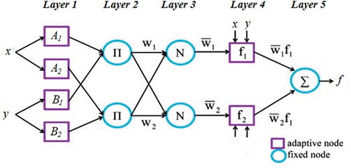
where A₁, A₂ and B₁, B₂ are membership funcctions (MF) for inputs x and y, respectively; and p₁, q₁, r₁ and p₂, q₂, r₂ are parameters of the output function.

In the first layer, all input variables provide the class membership with the MF and in Layer 2, all membership classes are multiplied together. In Layer 3, the entire classes of members are normalized and in Layer 4, the involvement of all rules is calculated. In the final layer (Layer 5), the target variable is calculated as the weighted average of class membership (Parsaie et al. 2017b, Sihag et al. 2017c, Tiwari et al. 2018, Tiwari and Sihag 2018).

The ANFIS has two learning algorithms, hybrid and back-propagation methods, which try to minimize the error among the actual and estimated values. The ANFIS model is able to solve any complex or non-linear problems with high accuracy. In this study, an ANFIS model was designed for estimating the infiltration process in arid regions of Iran.

2.2 Support vector machine (SVM)

Vapnik (1995) recommended the use of support vector regression, which entails choosing a ε -insensitive loss function. The loss function permits the idea of a margin amid two classes to be used. The margin is demonstrated as the gap between the two distinct classes and hyperplane. The primary intention of SVM is to perceive a function which presents the utmost ε deviation relative to the actual target vector for the input training set and is prone to making it as flat as possible (Cortes and Vapnik 1995). Vapnik proposed the use of kernel tricks to work out nonlinear SVM based regression. For further details on SVM, the reader is referred to Vapnik (1999) and Smola and Schölkopf (2004).

The performance of SVM methods relies upon the appropriate selection of kernel functions, which are finalized after a number of trials on different kernels. Three kernels were finalized, i.e the polynomial kernel, the radial basis kernel (RBF) and the Pearson VII universal kernel function (PUK), which are expressed as follows:

Polynomial kernel:

(1) $K\left(x_i,x_j\right)={{\left(\left(x_i.x_j\right)+1\right)}^d}^{\ast }$(1)

Radial basis kernel (RBF): (2)

PUK kernel:

(3) $K\left(x_i{x}_j\right)=\frac{1}{{\left[1+{\left(\frac{2\sqrt{\parallel }{x}_i-x_j{\parallel }^2\sqrt{2^{\frac{1}{\omega }}\text{-}1}}{\sigma }\right)}^2\right]}^{\omega }}$(3)

The performance of these kernels relies on the setting of control variables. The values of C, d*, ω, σ and γ are the primary parameters of the models.

The main limitations of SVM are overfitting and the selection of a suitable kernel function. The SVM model is time-consuming for large datasets and it is difficult to understand and interpret the final model, variable weights and individual impact, since the final model is not so easy to see and one cannot do small calibrations to the model.

2.3 Random forest (RF)

The random forest technique was introduced by Breiman (1999) and contains an assembly of several trees. Each tree represents a particular classification and chooses the classification. The random forest approach selects the classification which has a higher choice in the forest. The tree is mature if N is the number of cases in the training set. N cases at random with replacement from original data may be the input dataset to mature the tree. The design of random forest regression allows a tree to grow up to a maximum height of new training data using the mixing of variables. The m variables are selected randomly out of K input variables for the best split and the value of m should be less than K and fixed. A tree is developed up to a large extent without pruning. RF can effectively contain several input variables in a large and complex dataset.

The main limitation of RF is that a large number of trees can develop, making the algorithm too slow and unproductive for real-time estimations. In general, the RF algorithm is fast to train, but quite time-consuming to create estimations after training. A more precise estimation needs extra trees, which results in a slower model. In most real-world applications the random forest algorithm is fast enough, but there can certainly be situations where run-time performance is important and other approaches would be preferred.

2.4 Selection of the best fitting model

To asses the capability of the models, four performance statistics were estimated and the models with the best goodness-of-fit were chosen as the best ones. The performace criteria, correlation coefficient (CC), coefficient of determination (R²), root mean square error (RMSE) and Nash-Sutcliffe efficiency (NSE) were calculated as follows:

(4) $\mathrm{C}\mathrm{C}=\frac{N\sum OP-(\sum O)(\sum P)}{\sqrt{N(\sum O^2)-{(\sum O)}^2}\sqrt{N(\sum P^2)-{(\sum P)}^2}}$(4)

(5) $R^2={\left[\frac{N\sum OP-(\sum O)(\sum O)}{\sqrt{N(\sum O^2)-{(\sum O)}^2}\sqrt{N(\sum P^2)-{(\sum P)}^2}}\right]}^2$(5)

(6) $\mathrm{R}\mathrm{M}\mathrm{S}\mathrm{E}=\sqrt{\frac{1}{N}\left({\sum }_{i=1}^N{\left(P-O\right)}^2\right)}$(6)

(7) $\mathrm{N}\mathrm{S}\mathrm{E}=1-\frac{{\sum }_{i=1}^N{\left(O-P\right)}^2}{{\sum }_{i=1}^N{\left(O-\bar{O}\right)}^2}$(7)

where O and P are the observed and predicted values, respectively; N is the number of observations and $\bar{O}$ is the average of observed values.

3 Materials and methods

3.1 Study area

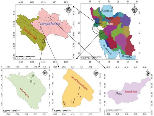
This study was carried out on bare land areas in western Iran: the Davood Rashid (47°41′34.21″E, 33°33′30.31″N) and Honam (48°16′41.97″E, 33°47′20.01″N) regions in Lorestan Province, and the Kelat region (47°50′38.97″E, 32°38′26.37″N) in Ilam Province. The study areas are shown in Fig. 2.

Figure 2. Location of the study area and sampling points.

3.2 Methodology

Infiltration data were collected using a double-ring infiltrometer of 30 cm and 60 cm diameter, consisting of two concentric rings with 30 cm depth. The infiltrometer was gently driven into the soil up to 10 cm depth. The rings were fixed in location with the least interruption of the soil surface. Both rings were filled with water at the same level and the primary water level was recorded. Then, cumulative infiltration of water vs time was monitored. For each sample, the infiltration experiments were continued until the infiltration rate reached a steady value. The infiltration rate was then calculated from the measured cumulative infiltration data. In order to measure the bulk density (BD) and the soil moisture content, an undisturbed soil sample was collected from the surface (near to the fixed infiltrometer), using a core sampler of 10.5 cm diameter and 11.54 cm height (i.e. 1000 cm³). The soil moisture content was determined by the gravimetric method. The observations of initial and final infiltration rate and properties of the soil for all the sites are listed in Table 1.

Table 1. Soil and hydraulic properties of sample sites 1–16. Init. inf.: initial infiltration rate; Steady inf.: steady infiltration rate. C: clay; Si: silt; S: sand; D: density; W: moisture content.

Property	1	2	3	4	5	6	7	8	9	10	11	12	13	14	15	16
Init. inf.	0.32	0.32	0.36	0.36	0.64	0.56	0.6	0.12	0.8	0.44	0.44	0.76	0.48	0.36	1.48	1.56
Steady inf.	0.15	0.11	0.13	0.14	0.28	0.2	0.2	0.08	0.24	0.1	0.14	0.14	0.16	0.12	0.38	0.38
C (%)	10	12	12	14	26	25	16	18	28	16	18	20	24	52	50	42
Si (%)	52	58	50	50	44	49	51	62	55	65	53	51	49	37	44	37
S (%)	38	30	38	36	30	26	33	20	17	19	29	29	27	11	6	21
D (g/cm^3)	1.42	1.42	1.79	1.63	1.44	1.45	1.4	1.08	1.3	1.27	1.4	1.24	1.32	1.56	1.46	1.48
W (%)	2.73	3.08	2.58	2.49	2.37	2.37	2.48	3.84	2.24	1.66	2.18	1.71	1.95	2.42	2.3	2.3

3.3 Data analysis

The dataset contains measurable soil and hydraulic properties,including variables, time (t), sand (S), clay (C), silt (Si), soil density (D), soil moisture (W), cumulative infiltration (F(t)), and infiltration rate (f(t)), which were measured or calculated at 16 different locations in the study areas in western Iran (Section 3.1). The complete dataset and features are listed in the Supplementary material, Table S1. Table 2 presents the input variables and input combinations considered for modelling of cumulative infiltration and infiltration rate. Accordingly, 10 models were considered; 70% of the data was selected for training the models and the remaining 30% was used for testing.

Table 2. Selecting different models for modelling of cumulative infiltration and infiltration rate.

Serial no.	Input combination	Cumulative infiltration		Infiltration rate
		Models	Output	Models	Output
1	t	C1	F(t)	M1	f(t)
2	t + D	C2	F(t)	M2	f(t)
3	t + D + W	C3	F(t)	M3	f(t)
4	t + S + D	C4	F(t)	M4	f(t)
5	t + S + D + W	C5	F(t)	M5	f(t)
6	t + S + C + W	C6	F(t)	M6	f(t)
7	t + S + C + W + D	C7	F(t)	M7	f(t)
8	t + S + C+ Si+W	C8	F(t)	M8	f(t)
9	t + S + C+ Si+D	C9	F(t)	M9	f(t)
10	t + S + C+ Si+D + W	C10	F(t)	M10	f(t)

3.4 Model implementation

This was the first attempt to implement the ANFIS models for estimating the infiltration process. The SVM, RF and ANFIS techniquest are believed to be able to capture the relationships among the inputs and output after training with actual data.

In this study, preparing the models comprised several steps. First, the input data (sand, silt, clay, density and moisture content) were analysed in detail. The more accurate the selected inputs are, the more realistic the infiltration estimation will be. The SVM was created and configured using the WEKA 3.9 software. Considering the different characteristics of the problem, the most suitable user-defined parameters were selected after a trial-and-error procedure. After experimenting with different training functions, the most suitable training function was chosen for the problem. The C, d*, omega, sigma and gamma values were determined through trial and error. Preparation of the RF model is similar to the SVM model. In the RF model, the number of features (k) and instances (I) were determined through trial and error.

The ANFIS model was designed and trained by using MATLAB 2013b software, ANFIS designer. For the ANFIS interpretation, the Sugeno Inference System was chosen. In the ANFIS structure, the implication of the errors is different from that of the RF and SVM. In order to find the optimal result, the epoch size is not limited. The parameters were optimized after numerous trials. In the ANFIS model four shapes of membership functions – triangular (trimf), trapezoidal (tramf), generalized bell shape (gbell) and Gaussian – were used in model development with a hybrid algorithm.

The model was trained numerous times until the required precision level was achieved and the error minimized. The four statistical parameters (CC, R², RMSE and NSE; Section 2.4) were used to evaluate the performance of the developed models. The training data (70% of the dataset) was selected for training the SVM, RF and ANFIS models, and the testing data (30%) was used to evaluate the performance of the developed models.

4 Results and discussion

4.1 ANFIS

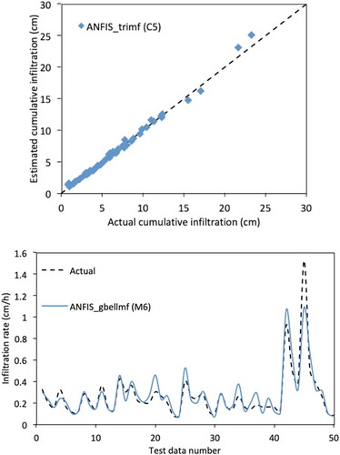
The ANFIS model was implemented using MATLAB 2013a software. Developing the Sugeno fuzzy rule-based ANFIS is a trial-and-error process based on the data (Supplementary material, Table S1); the dataset was separated into two parts for training and testing. The shapes of MFs, which have the best performance with the models, are given in Table 3. For estimating cumulative infiltration, the ANFIS model C5 (Table 2) with triangular function (trimf) performed better than other models in testing (CC = 0.9965, R² = 0.9931, RMSE = 0.4385 cm and NSE = 0.9921). For estimating infiltration rate, the ANFIS model M6 with generalized bell shape (gbell) (dependent variables time, sand, clay and moisture content of soil) performed better than the other models in testing (CC = 0.9239, R² = 0.8536, RMSE = 0.0887 cm/h and NSE = 0.8521). The performance of the best fit ANFIS models for cumulative infiltration and infiltration rate are shown in Figs. 3 and 4, respectively. The overall performance of the ANFIS model is suitable for estimating the cumulative infiltration and infiltration rate of the soil.

Table 3. Performance assessment using ANFIS based models. MF: membership function. The best-fit models are indicated by bold values. Membership functions (MF): trimf: triangular; tramf: trapezoidal; gbell: generalized bell shape.

Model	MF	Training dataset			Testing dataset
		CC	R^2	RMSE	NSE	CC	R^2	RMSE	NSE
Cumulative infiltration
C1	trimf	0.6323	0.3998	4.4630	0.3998	0.5943	0.3532	4.0257	0.3329
C2	Gaussian	0.7329	0.5371	3.9194	0.5371	0.7101	0.5042	3.5732	0.4745
C3	tramf	0.8058	0.6494	3.4113	0.6494	0.7781	0.6055	3.2085	0.5763
C4	trimf	0.9793	0.9591	1.1656	0.9591	0.9758	0.9522	1.0942	0.9507
C5	trimf	0.9976	0.9952	0.4003	0.9952	0.9965	0.9931	0.4385	0.9921
C6	Gaussian	0.9907	0.9815	0.7842	0.9815	0.9906	0.9813	0.6848	0.9807
C7	trimf	0.9976	0.9952	0.4002	0.9952	0.9962	0.9925	0.4582	0.9914
C8	Gaussian	0.9905	0.9810	0.7936	0.9810	0.9901	0.9802	0.7058	0.9795
C9	Gaussian	0.9925	0.9851	0.7029	0.9851	0.9946	0.9892	0.5160	0.9890
C10	trimf	0.9976	0.9952	0.4002	0.9952	0.9963	0.9927	0.4532	0.9915
Infiltration rate
M1	trimf	0.4916	0.2416	0.2067	0.2416	0.4453	0.1983	0.2065	0.1927
M2	Gaussian	0.5935	0.3523	0.1910	0.3523	0.5712	0.3262	0.1895	0.3198
M3	Gaussian	0.8834	0.7803	0.1112	0.7803	0.7225	0.5220	0.1592	0.5204
M4	gbell	0.8656	0.7493	0.1188	0.7493	0.9188	0.8442	0.0912	0.8425
M5	trimf	0.9278	0.8608	0.0885	0.8608	0.9186	0.8437	0.0922	0.8391
M6	gbell	0.8897	0.7916	0.1084	0.7916	0.9239	0.8536	0.0887	0.8511
M7	trimf	0.9278	0.8608	0.0885	0.8608	0.9182	0.8431	0.0925	0.8382
M8	gbell	0.8894	0.7911	0.1085	0.7911	0.9233	0.8525	0.0890	0.8499
M9	gbell	0.8916	0.7949	0.1075	0.7949	0.9189	0.8443	0.0913	0.8422
M10	trimf	0.9278	0.8608	0.0885	0.8608	0.9181	0.8429	0.0925	0.8380

Figure 3. Performance of C5 triangular membership function-based ANFIS model for cumulative infiltration of soil – testing dataset.

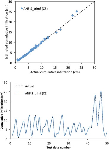
Figure 4. Performance of M6 generalized bell shape membership function-based ANFIS model for infiltration rate of soil – testing dataset.

4.2 SVM

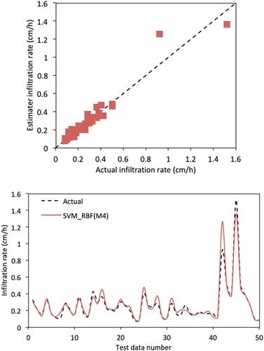
The SVM model was implemented using WEKA 3.9 software. Three kernel functions were used in this study. Table 4 presents the results obtained (CC, R² and RMSE) by the SVM models for cumulative infiltration and infiltration rate. For estimating cumulative infiltration, the performance criteria show that the SVM model C10 with RBF (dependent variables time, sand, clay, silt, density of soil, soil moisture content) performed better than other models in testing (CC = 0.9984, R² = 0.9969, RMSE = 0.2781 cm and NSE = 0.9968). For estimating infiltration rate, the SVM model M4 with RBF (dependent variables time, sand, density) performed better than other models in testing (CC = 0.9650, R² = 0.9312, RMSE = 0.0631 cm/h and NSE = 0.9246). The performance of best-fit SVM model for cumulative infiltration and infiltration rate is shown in Figs. 5 and 6, respectively. Overall, the SVM model is suitable for estimating cumulative infiltration and infiltration rate.

Table 4. Performance assessment of SVM based models. The best-fit models are indicated by bold values.

Model	Kernel function	Training dataset			Testing dataset
		CC	R^2	RMSE	NSE	CC	R^2	RMSE	NSE
Cumulative infiltration
C1	PUK	0.6274	0.3937	4.7310	0.3256	0.5707	0.3257	4.1741	0.2828
C2	PUK	0.7286	0.5308	4.1039	0.4925	0.6863	0.4710	3.6386	0.4550
C3	RBF	0.9242	0.8541	2.2516	0.8472	0.7794	0.6074	3.1753	0.5850
C4	RBF	0.9941	0.9882	0.6425	0.9876	0.9917	0.9835	0.6470	0.9828
C5	RBF	0.9999	0.9999	0.0615	0.9999	0.9981	0.9963	0.3021	0.9962
C6	RBF	0.9961	0.9922	0.5233	0.9917	0.9946	0.9892	0.5150	0.9891
C7	RBF	0.9999	0.9997	0.0919	0.9997	0.9983	0.9966	0.2911	0.9965
C8	RBF	0.9965	0.9930	0.4929	0.9927	0.9942	0.9885	0.5326	0.9883
C9	RBF	0.9980	0.9959	0.3692	0.9959	0.9961	0.9921	0.4412	0.9920
C10	RBF	0.9999	0.9998	0.0851	0.9998	0.9984	0.9969	0.2791	0.9968
Infiltration rate
M1	PUK	0.5582	0.3115	0.2060	0.2467	0.5037	0.2538	0.2045	0.2082
M2	PUK	0.6800	0.4624	0.1869	0.3798	0.5916	0.3499	0.1905	0.3126
M3	RBF	0.9851	0.9704	0.0441	0.9655	0.9022	0.8139	0.1023	0.8019
M4	RBF	0.9685	0.9380	0.0592	0.9377	0.9650	0.9312	0.0631	0.9246
M5	RBF	0.9764	0.9534	0.0516	0.9526	0.9581	0.9180	0.0708	0.9050
M6	RBF	0.9723	0.9453	0.0561	0.9441	0.9530	0.9082	0.0708	0.9050
M7	RBF	0.9908	0.9817	0.0330	0.9807	0.9507	0.9038	0.0764	0.8894
M8	PUK	1.0000	1.0000	0.0017	0.9999	0.9427	0.8886	0.0809	0.8761
M9	RBF	0.9867	0.9736	0.0386	0.9735	0.9565	0.9149	0.0699	0.9075
M10	PUK	1.0000	1.0000	0.0017	0.9999	0.9513	0.9050	0.0755	0.8921

Figure 5. Performance of C10 RBF kernel function-based SVM model for cumulative infiltration of soil – testing dataset.

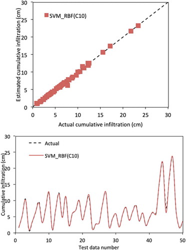
Figure 6. Performance of M4 RBF kernel function-based SVM model for infiltration rate of soil – testing dataset.

4.3 RF

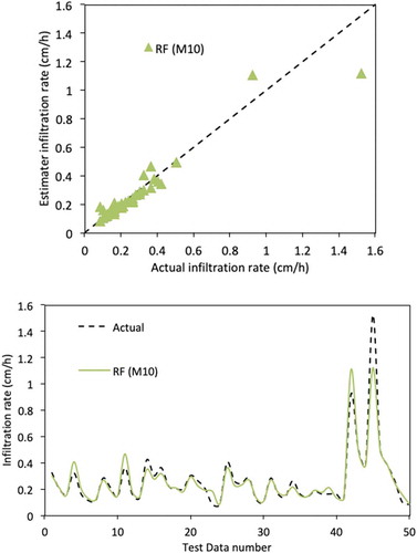
The RF model was also implemented using WEKA 3.9 software and it is the same as the SVM model. The optimum values of the primary parameters (k = 10, m = 1 and I = 100) were kept constant for comparison among models. Three kernel functions were used in this study. Table 5 presents the results obtained (CC, R² and RMSE) by RF models for cumulative infiltration and infiltration rate. The performance criteria show that RF-based models C10 and M10 (dependent variables time, sand, clay, silt, density of soil, soil moisture content) performed better than other models in testing for estimating the cumulative infiltration (CC = 0.9824, R² = 0.9650, RMSE = 0.9677 cm and NSE = 0.9615) and for estimating infiltration rate (CC = 0.9650, R² = 0.9123, RMSE = 0.0707 cm/h and NSE = 0.9054). The performance of the best fit RF model for cumulative infiltration and infiltration rate of soil is shown in Figs. 7 and 8, respectively. The overall performance of the RF model was suitable for estimating cumulative infiltration and infiltration rate.

Table 5. Performance assessment of RF-based models for cumulative and infiltration rate. The best-fit models are indicated by bold values.

Model	Training dataset				Testing dataset
	CC	R^2	RMSE	NSE	CC	R^2	RMSE	NSE
Cumulative infiltration
C1	0.6783	0.4601	4.2333	0.4600	0.4083	0.1667	4.9425	−0.0055
C2	0.9876	0.9754	0.9886	0.9706	0.8598	0.7392	2.6231	0.7168
C3	0.9874	0.9749	0.9904	0.9704	0.8298	0.6886	2.7590	0.6867
C4	0.9961	0.9922	0.5304	0.9915	0.9754	0.9515	1.1259	0.9478
C5	0.9969	0.9937	0.4836	0.9930	0.9813	0.9629	0.9908	0.9596
C6	0.9964	0.9927	0.5193	0.9919	0.9784	0.9573	1.0931	0.9508
C7	0.9969	0.9939	0.4787	0.9931	0.9822	0.9647	0.9738	0.9610
C8	0.9964	0.9927	0.5168	0.9920	0.9785	0.9575	1.0896	0.9511
C9	0.9963	0.9925	0.5187	0.9919	0.9776	0.9558	1.0809	0.9519
C10	0.9969	0.9938	0.4792	0.9931	0.9824	0.9650	0.9677	0.9615
Infiltration rate
M1	0.6241	0.3895	0.1856	0.3885	0.1608	0.0258	0.2340	−0.0368
M2	0.9549	0.9119	0.0738	0.9032	0.8138	0.6622	0.1468	0.5919
M3	0.9572	0.9163	0.0748	0.9007	0.8438	0.7120	0.1414	0.6216
M4	0.9879	0.9759	0.0402	0.9713	0.9500	0.9024	0.0737	0.8973
M5	0.9867	0.9735	0.0418	0.9689	0.9535	0.9091	0.0713	0.9038
M6	0.9864	0.9730	0.0423	0.9682	0.9525	0.9072	0.0725	0.9005
M7	0.9855	0.9713	0.0432	0.9668	0.9540	0.9102	0.0713	0.9038
M8	0.9861	0.9724	0.0430	0.9672	0.9534	0.9090	0.0720	0.9018
M9	0.9875	0.9751	0.0411	0.9700	0.9560	0.9139	0.0708	0.9050
M10	0.9857	0.9716	0.0431	0.9670	0.9551	0.9123	0.0707	0.9054

Figure 7. Performance of C10 RF model for cumulative infiltration of soil – testing dataset.

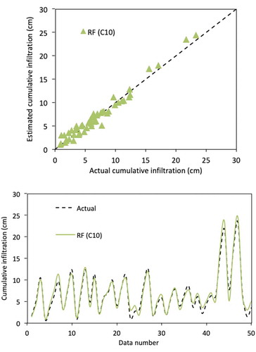
Figure 8. Performance of M10 RF model for infiltration rate of soil – testing dataset.

4.4 Comparison of models

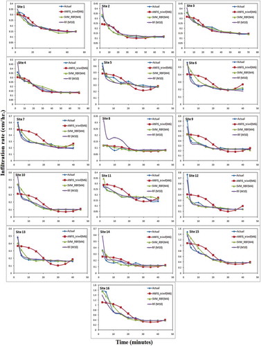
Table 6 and Figs. 9 and 11 suggest that the RBF-based SVM models worked better than the ANFIS and RF-based models. Model C10 (dependent variables time, sand, clay, silt, density of soil, soil moisture content) and M4 (dependent variables time, sand, density) performed better than the models based on other input combinations for cumulative infiltration and infiltration rate, respectively. Figures 10 and 12 show the actual and estimated curves of 16 sites using the ANFIS, SVM and RF-based models for cumulative infiltration and infiltration rate, respectively. While Figs. 9 and 11 indicate that estimated values using the RBF-based SVM model were closer to the line of perfect agreement for cumulative infiltration and infiltration rate, respectively, Figs. 10 and 12 indicate that estimated values using the RBF-based SVM model followed the same path as followed by actual values of cumulative infiltration and infiltration rate, respectively.

Table 6. Results of different modelling approaches for cumulative infiltration and infiltration rate. The best-fit models are indicated by bold values.

Model	AI-based technique	MF/kernel function	Training dataset				Testing dataset
			CC	R^2	RMSE	NSE	CC	R^2	RMSE	NSE
Cumulative infiltration
C5	ANFIS	trimf	0.9976	0.9952	0.4003	0.9952	0.9965	0.9931	0.4385	0.9921
C10	SVM	RBF	0.9999	0.9998	0.0851	0.9998	0.9984	0.9969	0.2791	0.9968
C10	RF	-	0.9969	0.9938	0.4792	0.9931	0.9824	0.965	0.9677	0.9615
Infiltration rate
M6	ANFIS	gbell	0.8897	0.7916	0.1084	0.7916	0.9239	0.8536	0.0887	0.8511
M4	SVM	RBF	0.9685	0.938	0.0592	0.9377	0.965	0.9312	0.0631	0.9246
M10	RF	-	0.9857	0.9716	0.0431	0.9670	0.9551	0.9123	0.0707	0.9054

Figure 9. Agreement of actual and estimated values of cumulative infiltration of soil using ANFIS, SVM and RF-based models – testing period.

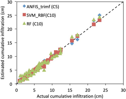
Figure 10. Actual and estimated cumulative infiltration curves of the 16 study sites using ANFIS, SVM and RF-based models.

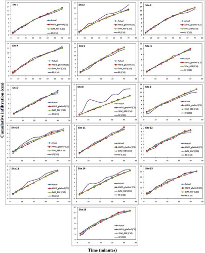
Figure 11. Agreement plot of actual and estimated values of infiltration rate using ANFIS, SVM and RF-based models – testing period.

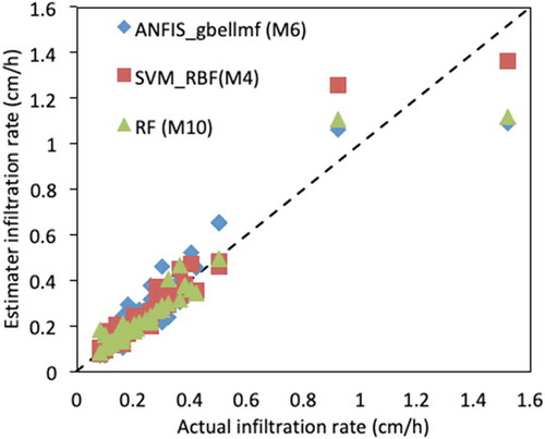
Figure 12. Actual and estimated infiltration rate curves of the 16 study sites using ANFIS, SVM and RF-based models.

4.5 Sensitivity analysis

The most effective parameters for estimating of infiltration process by SVM were defined via a simple approach. This approach describes the effect of each parameter on model performance to estimate the output (Mehdipour et al. 2018). First, regarding models C10 and M4, all parameters are considered as inputs for SVM. Then, one of the input parameters is removed from and again the model is prepared with the same structure. It is notable that the models were considered regarding the same user-defined parameters as desribed in the model development section. The performance of the models in the absence of one input parameter at a time was assessed using the error indices CC and RMSE. Clearly, removing one of the input parameters resulted in a change in model performance. Depending on the severity of such change, the effect of each parameter can be assessed. The results of the sensitivity analysis of SVM are given in Tables 7 and 8 for cumulative infiltration and infiltration rate, respectively. As may be seen in Table 7, the absence of time (t) causes a dramatic decrease in the accuracy of models; therefore, this parameter is considered the most important one for modelling cumulative infiltration of soil. In Table 8 the absence of sand (S, %) and time (t) caused a dramatic decrease in the accuracy of the M4 SVM based models; therefore, it these parameters are considered the most essential ones for modelling the infiltration rate of soil for this dataset.

Table 7. Sensitivity analysis using C10 SVM_RBF for cumulative infiltration. The best fit is indicated by bold values.

Input combination	Input parameter removed	SVM_RBF
		CC	RMSE
t, S, C, Si, D, W		0.9984	0.2791
S, C, Si, D, W	t	0.6752	3.853
t, C, Si, D, W	S	0.9984	0.2775
t, S, Si, D, W	C	0.998	0.3083
t, S, C, D, W	Si	0.9983	0.2935
t, S, C, Si, W	D	0.9911	0.6674
t, S, C, Si, D	W	0.9844	0.8721

Table 8. Sensitivity analysis using SVM_RBF. The best fit is indicated by bold values.

Input combination	Input parameter removed	SVM_RBF
		CC	RMSE
t, S, D		0.9650	0.0631
S, D	t	0.7233	0.1729
t, D	S	0.5728	0.1916
t, S	D	0.9312	0.0869

5 Conclusions

In this study, ANFIS, SVM and random forest models were used for estimating cumulative infiltration and infiltration rate in arid regions in Iran. Comparison of these models showed that the C10 SVM_RBF model, with the combination of time, sand, clay, silt, soil density and soil moisture, could estimate cumulative infiltration with much less error than the other models. The results of the performance assessment showed that the M4 SVM_RBF model, with the combination of time, sand and soil density, performed better than other models for estimating infiltration rate. Sensitivity analysis suggest that time (t) is the most important parameter in estimating cumulative infiltration, whereas time and percentage of sand are the most essential parameters for estimating infiltration rate using SVM-based modelling for the arid regions of Iran.

Disclosure statement

No potential conflict of interest was reported by the authors.

Supplementary material

Supplementary data for this article can be accessed here.

References

- Achari, M.S., Dhakshinamurthy, M., and Arunachalam, G., 1999. Studies of the influence on paper mill effluents on the yield, availability and uptake of nutrients in rice. Journal of the Indian Society of Soil Science, 47 (2), 276–280.
- Al-Sulaiman, M.A., 2015. Applying of an adaptive neuro fuzzy inference system for prediction of unsaturated soil hydraulic conductivity. Biosciences, Biotechnology Research Asia, 12 (3), 2261–2272. doi:10.13005/bbra/1899
- Anari, P.L., Darani, H.S., and Nafarzadegan, A.R., 2011. Application of ANN and ANFIS models for estimating total infiltration rate in an arid rangeland ecosystem. Research Journal of Environmental Sciences, 5 (3), 236. doi:10.3923/rjes.2011.236.247
- Angelaki, A., et al., 2018. Estimation of models for cumulative infiltration of soil using machine learning methods. ISH Journal of Hydraulic Engineering, 1–8. doi:10.1080/09715010.2018.1531274
- Angelaki, A., Sakellariou-Makrantonaki, M., and Tzimopoulos, C., 2013. Theoretical and experimental research of cumulative infiltration. Transport in Porous Media, 100 (2), 247–257. doi:10.1007/s11242-013-0214-2
- Arshad, M., Shoaib, A., and Beg, I., 2013. Fixed point of a pair of contractive dominated mappings on a closed ball in an ordered dislocated metric space. Fixed Point Theory and Applications, 2013 (1), 115. doi:10.1186/1687-1812-2013-115
- Azamathulla, H.M., Haghiabi, A.H., and Parsaie, A., 2016. Prediction of side weir discharge coefficient by support vector machine technique. Water Science and Technology: Water Supply, 16 (4), 1002–1016.
- Babaei, F., et al., 2018. Spatial analysis of infiltration in agricultural lands in arid areas of Iran. CATENA, 170, 25–35. doi:10.1016/j.catena.2018.05.039
- Breiman, L., 1999. Random forests. Berkeley, CA: University of Calfornia at Berkeley, Reoprt TR567.
- Corradini, C., Melone, F., and Smith, R.E., 1994. Modeling infiltration during complex rainfall sequences. Water Resources Research, 30 (10), 2777–2784. doi:10.1029/94WR00951
- Cortes, C. and Vapnik, V., 1995. Support-vector networks. Machine Learning, 20 (3), 27297. doi:10.1007/BF00994018
- Das, L., et al., 2011. Centennial scale warming over Japan: are the rural stations really rural? Atmospheric Science Letters, 12 (4), 362–367. doi:10.1002/asl.v12.4
- Elbisy, M.S., 2015. Support Vector Machine and regression analysis to predict the field hydraulic conductivity of sandy soil. KSCE Journal of Civil Engineering, 19 (7), 2307–2316. doi:10.1007/s12205-015-0210-x
- Erzin, Y., et al., 2009. Artificial neural network (ANN) models for determining hydraulic conductivity of compacted fine-grained soils. Canadian Geotechnical Journal, 46 (8), 955–968. doi:10.1139/T09-035
- Green, W.H. and Ampt, G.A., 1911. Studies on soil phyics. The Journal of Agricultural Science, 4 (1), 1–24. doi:10.1017/S0021859600001441
- Holtan, H.N., 1961. Concept for infiltration estimates in watershed engineering. Washington, DC: US Department of Agriculture.
- Horton, R.E., 1941. An approach toward a physical interpretation of infiltration-capacity 1. Soil Science Society of America Journal, 5 (C), 399–417. doi:10.2136/sssaj1941.036159950005000C0075x
- Kostiakov, A.N., 1932. On the dynamics of the coefficient of water percolation in soils and the necessity of studying it from the dynamic point of view for the purposes of amelioration. Transactions of the Sixth Committee of the International Society of Soil Science, 1, 7–21.
- Kumar, M. and Sihag, P., 2019. Assessment of infiltration rate of soil using empirical and machine learning‐based models. Irrigation and Drainage, 68, 588–601. doi:10.1002/ird.2332
- Kumar, M., Sihag, P., and Singh, V., 2019. Enhanced soft computing for ensemble approach to estimate the compressive strength of high strength concrete. Journal of Materials and Engineering Structures, JMES, 6 (1), 93–103.
- Loague, K. and Gander, G.A., 1990. R‐5 revisited: 1. Spatial variability of infiltration on a small rangeland catchment. Water Resources Research, 26 (5), 957–971. doi:10.1029/WR026i005p00957
- Mehdipour, V., et al., 2018. Comparing different methods for statistical modeling of particulate matter in Tehran, Iran. Air Quality, Atmosphere & Health, 11 (10), 1155–1165. doi:10.1007/s11869-018-0615-z
- Mohanty, S., et al., 2019. Estimating the strength of stabilized dispersive soil with cement clinker and fly ash. Geotechnical and Geological Engineering, 37 (4), 1–12. doi:10.1007/s10706-019-00808-1
- Nain, S.S., Sihag, P., and Luthra, S., 2018. Performance evaluation of fuzzy-logic and BP-ANN methods for WEDM of aeronautics super alloy. MethodsX, 5, 890–908. doi:10.1016/j.mex.2018.04.006
- Parlange, J.Y., 1971a. Theory of water movement in soils: 1. One-dimensional absorption. Soil Science, 111 (2), 134–137. doi:10.1097/00010694-197102000-00010
- Parlange, J.Y., 1971b. Theory of water movement in soils: 2. One-imensional infiltration. Soil Science, 111 (3), 170–174. doi:10.1097/00010694-197103000-00004
- Parlange, J.Y., 1972a. Theory of water movement in soils. 6. Effect of water depth over soil. Soil Science, 133, 308–312. doi:10.1097/00010694-197205000-00002
- Parlange, J.Y., 1972b. Theory of water movement in soils. 8. One-dimensional infiltration with constant flux at the surface. Soil Science, 114, 1–4. doi:10.1097/00010694-197207000-00001
- Parlange, J.Y., 1975. A note of the Green & Ampt equation. Soil Science, 119, 466–467. doi:10.1097/00010694-197506000-00009
- Parlange, J.Y., et al., 1982. The three parameter infiltration equation. Soil Science, 133, 337–341. doi:10.1097/00010694-198206000-00001
- Parlange, J.Y., Havercamp, R., and Touma, J., 1985. Infiltration under ponded conditions: 1. Optimal analytical solution and comparison with experimental observations. Soil Science, 139, 305–311. doi:10.1097/00010694-198504000-00003
- Parsaie, A., et al., 2017b. Predication of discharge coefficient of cylindrical weir-gate using adaptive neuro fuzzy inference systems (ANFIS). Frontiers of Structural and Civil Engineering, 11 (1), 111–122. doi:10.1007/s11709-016-0354-x
- Parsaie, A., Yonesi, H., and Najafian, S., 2017a. Prediction of flow discharge in compound open channels using adaptive neuro fuzzy inference system method. Flow Measurement and Instrumentation, 54, 288–297. doi:10.1016/j.flowmeasinst.2016.08.013
- Philip, J.R., 1957a. Theory of infiltration: 1. The infiltration equation and its solution. Soil Science, 83, 435–448. doi:10.1097/00010694-195706000-00003
- Philip, J.R., 1957b. Theory of infiltration: 4. Sorptivity and algebraic infiltration equations. Soil Science, 84, 257–264. doi:10.1097/00010694-195709000-00010
- Rahmati, M., 2017. Reliable and accurate point-based prediction of cumulative infiltration using soil readily available characteristics: a comparison between GMDH, ANN, and MLR. Journal of Hydrology, 551, 81–91. doi:10.1016/j.jhydrol.2017.05.046
- Schaap, M.G. and Leij, F.J., 1998. Using neural networks to predict soil water retention and soil hydraulic conductivity. Soil and Tillage Research, 47 (1–2), 37–42. doi:10.1016/S0167-1987(98)00070-1
- SCS (Soil Conservation Service), 1972. National engineering handbook, section 4: hydrology. Washington, DC: Department of Agriculture, 762.
- Sepahvand, A., et al., 2019. Assessment of the various soft computing techniques to predict sodium absorption ratio (SAR). ISH Journal of Hydraulic Engineering, 1–12. doi:10.1080/09715010.2019.1595185
- Sihag, P., 2018. Prediction of unsaturated hydraulic conductivity using fuzzy logic and artificial neural network. Modeling Earth Systems and Environment, 4 (1), 189–198. doi:10.1007/s40808-018-0434-0
- Sihag, P., et al., 2018a. Modeling the infiltration process with soft computing techniques. ISH Journal of Hydraulic Engineering, 1–15. doi:10.1080/09715010.2018.1464408
- Sihag, P., et al., 2019a. Modeling unsaturated hydraulic conductivity by hybrid soft computing techniques. Soft Computing, 1–14. doi:10.1007/s00500-019-03847-1
- Sihag, P., et al., 2019b. Model-based soil temperature estimation using climatic parameters: the case of Azerbaijan Province, Iran. Geology, Ecology, and Landscapes, 1–13. doi:10.1080/24749508.2019.1610841
- Sihag, P., Jain, P., and Kumar, M., 2018b. Modeling of impact of water quality on recharging rate of storm water filter system using various kernel function based regression. Modelling Earth Systems and Environment, 4 (1), 61–68. doi:10.1007/s40808-017-0410-0
- Sihag, P., Tiwari, N.K., and Ranjan, S., 2017a. Estimation and inter-comparison of infiltration models. Water Science, 31 (1), 34–43. doi:10.1016/j.wsj.2017.03.001
- Sihag, P., Tiwari, N.K., and Ranjan, S., 2017b. Modelling of infiltration of sandy soil using gaussian process regression. Modeling Earth Systems and Environment, 3 (3), 1091–1100. doi:10.1007/s40808-017-0357-1
- Sihag, P., Tiwari, N.K., and Ranjan, S., 2017c. Prediction of unsaturated hydraulic conductivity using adaptive neuro-fuzzy inference system (ANFIS). ISH Journal of Hydraulic Engineering, 1–11. doi:10.1080/09715010.2017.1381861
- Sihag, P., Tiwari, N.K., and Ranjan, S., 2018c. Support vector regression-based modeling of cumulative infiltration of sandy soil. ISH Journal of Hydraulic Engineering, 1–7. doi:10.1080/09715010.2018.1439776
- Singh, B., et al., 2018a. Estimation of trapping efficiency of vortex tube silt ejector. International Journal of River Basin Management, 1–38. doi:10.1080/15715124.2018.1476367
- Singh, B., Sihag, P., and Deswal, S., 2019. Modelling of the impact of water quality on the infiltration rate of the soil. Applied Water Science, 9 (1), 15. doi:10.1007/s13201-019-0892-1
- Singh, B., Sihag, P., and Singh, K., 2017. Modelling of impact of water quality on infiltration rate of soil by random forest regression. Modeling Earth Systems and Environment, 3 (3), 999–1004. doi:10.1007/s40808-017-0347-3
- Singh, B., Sihag, P., and Singh, K., 2018b. Comparison of infiltration models in NIT Kurukshetra campus. Applied Water Science, 8 (2), 63. doi:10.1007/s13201-018-0708-8
- Singh, V.P. and Yu, F.X., 1990. Derivation of infiltration equation using systems approach. Journal of Irrigation and Drainage Engineering, 116 (6), 837–858. doi:10.1061/(ASCE)0733-9437(1990)116:6(837)
- Smola, A.J. and Schölkopf, B., 2004. A tutorial on support vector regression. Statistics and Computing, 14 (3), 199–222. doi:10.1023/B:STCO.0000035301.49549.88
- Sy, N.L., 2006. Modelling the infiltration process with a multi-layer perceptron artificial neural network. Hydrological Sciences Journal, 51 (1), 3–20. doi:10.1623/hysj.51.1.3
- Taha, A., Gresillon, J.M., and Clothier, B.E., 1997. Modelling the link between hillslope water movement and streamflow: application to a small Mediterranean forest watershed. Journal of Hydrology, 203 (1–4), 11–20. doi:10.1016/S0022-1694(97)00081-4
- Takagi, T. and Sugeno, M., 1985. Fuzzy identification of systems and its application to modeling and control. IEEE Transaction on System, Man and Cybernetics, SMC-15, 116–132. doi:10.1109/TSMC.1985.6313399
- Tiwari, N.K., et al., 2018. Prediction of trapping efficiency of vortex tube ejector. ISH Journal of Hydraulic Engineering, 1–9. doi:10.1080/09715010.2018.1441752
- Tiwari, N.K., et al., 2019. Estimation of tunnel desilter sediment removal efficiency by ANFIS. Iranian Journal of Science and Technology, Transactions of Civil Engineering, 1–16. doi:10.1007/s40996-019-00261-3
- Tiwari, N.K. and Sihag, P., 2018. Prediction of oxygen transfer at modified Parshall flumes using regression models. ISH Journal of Hydraulic Engineering, 1–12. doi:10.1080/09715010.2018.1473058
- Tiwari, N.K., Sihag, P., and Ranjan, S., 2017. Modeling of infiltration of soil using adaptive neuro-fuzzy inference system (ANFIS). Journal of Engineering & Technology Education, 11 (1), 13–21.
- Vapnik, V.N., 1995. The nature of statistical learning theory. New York, NY: Springer-Verlag.
- Vapnik, V.N., 1999. An overview of statistical learning theory. IEEE Transactions on Neural Networks, 10 (5), 988–999. doi:10.1109/72.788640