Enhancing streamflow forecasting using the augmenting ensemble procedure coupled machine learning models: case study of Aswan High Dam

ABSTRACT

The potential of the most recent pre-processing tool, namely, complete ensemble empirical mode decomposition with adaptive noise (CEEMDAN), is examined for providing AI models (artificial neural network, ANN; M5-model tree, M5-MT; and multivariate adaptive regression spline, MARS) with more informative input–output data and, thence, evaluate their forecasting accuracy. A 130-year inflow dataset for Aswan High Dam, Egypt, is considered for training, validating and testing the proposed models to forecast the reservoir inflow up to six months ahead. The results show that, after the pre-processing analysis, there is a significant enhancement in the forecasting accuracy. The MARS model combined with CEEMDAN gave superior performance compared to the other models – CEEMDAN-ANN and CEEMDAN-M5-MT – with an increase in accuracy of, respectively, about 13–25% and 6–20% in terms of the root mean square error.

KEYWORDS:

• multi-lead-time forecasting
• reservoir inflow forecasting
• Aswan High Dam
• pre-processing analysis
• CEEMDAN

Editor A. Castellarin Associate editor F.-J. Chang

1 Introduction

1.1 Background

Streamflow or reservoir inflow forecasting models are of prime importance for decision-makers to optimally manage the available surface water resources. More specifically, accurate reservoir inflow forecasting models are beneficial for dam or reservoir managers to operate the water supply/distribution system effectively. The reservoir inflow monitoring is a routine task of many dam or barrage operating and maintenance organizations for possible forecasting of extreme events such as floods that damage the geomorphic and structural health of dams. First of all, streamflow monitoring via a stream gauging programme helps to analyse long-term and periodic changes in streamflow scenarios due to climate change; furthermore, it aids in furnishing water resource estimates for municipal water supply management. In addition, streamflow records are necessary for designing infrastructure, such as dams, reservoirs, bridges and culverts (Dobriyal et al. 2017).

Floods and droughts are the most significant of all natural hazards, being responsible for nearly 60% of fatalities from natural disasters (Giupponi et al. 2015). In recent years, the frequency and intensity of flood occurrences have increased owing to deforestation in the sphere of the watershed, changes in land-use patterns, farming practices and encroachment along the floodplain of rivers. In addition, the spatial patterns of rainfall, including its characteristics, such as time of occurrence, frequency, duration and magnitude, may influence the nature of streamflow patterns. Streamflow forecasts of sufficiently longer lead time may be of benefit for the efficient management of extreme events. Annual and seasonal streamflow forecasts are beneficial for reservoir and irrigation management, offering, for example, likelihood estimates of hydropower generation and quantification of climate variability by trend analysis.

Various research studies based on streamflow forecasting at multiple time scales are reported in the literature. Artificial intelligence (AI)-based models are gaining more popularity nowadays compared to numerical and physical process-oriented modelling approaches, due to their advantages, such as superior forecast efficiency, simpler or stress-free model building procedure and reduced computational time/effort. During the last two decades, AI-based models have shown outstanding performance in accurately forecast/predicting several hydrological variables. However, to date, multi-step-ahead forecasting of stochastic and non-linear data records, e.g. reservoir inflow, seems to be problematic even in the context of modelling using AI methods. The rationale could be the difficulty for AI methods to detect the high noise and dynamic changes in the time series data, especially of long-time data records. Therefore, to establish a successful multi-step-ahead forecasting model, there is a need to ideally provide the model with complete embedded features of the input–output pattern by utilizing appropriate multi-resolution data pre-processing tools.

1.2 Literature review: forecasting models

Inflow to any reservoir is mainly ascertained through stream gauging. Continuous stream gauging allows one to analyse the river regime and offers quantitative information for its utilization. It is indeed essential for several hydrological calculations and forecasts. The body of literature already covers several studies of streamflow forecasting, based on the complicated physical systems (Vieux et al. 2004, Rosenberg et al. 2011), numerical methods, such as finite difference approaches (Nwaogazie 1987, Clifford et al. 2009) and statistical methods such as auto-regressive moving average (ARMA) models (Mohammadi et al. 2006, Can et al. 2012) and advanced AI approaches (Abudu et al. 2010, Yaseen et al. 2015). The AI models have been demonstrated to provide more accurate estimates of streamflow at various time scales depending upon the user requirements (Kisi 2007, 2015, Vafakhah 2012, Shabri and Suhartono 2012). Over the years, several hybrid AI paradigms have also been proved to be feasible for detecting the non-linear and dynamic patterns of streamflow time series (Kisi 2009a, 2009b, Shiri and Kisi 2010, Humphrey et al. 2016). Unlike wavelet transforms, empirical mode decomposition (EMD) and ensemble empirical mode decomposition (EEMD) have gained immense interest in recent times due to their ease of analysing time-dependent nonlinear signals (Wang et al. 2018). Recently, an ensemble streamflow forecasting model, based on EMD and least absolute shrinkage and selection operator (Lasso), with deep belief networks (DBN), proposed and implemented by Chu et al. (2018), provided significantly improved monthly streamflow forecasts. Honorato et al. (2018) examined combinations of low-frequency components resulting from the wavelet decomposition as inputs to an ANN model. This hybrid model, when compared with classical ANN models of flow forecasting for 1, 3, 6 and 12 months ahead, showed superior accuracy, especially for the 1-, 3- and 6-step lead times.

Much of the past research on streamflow forecasting has been based on two quantitative modes: the first and more recurrent being the flow volume estimate over several time scales (daily, monthly, seasonal and long-term), and the second being categorical streamflow forecasting (low, medium and high flow probabilities) (Regonda et al. 2006). The reservoir decision support system needs to be evolved under anticipated conditions of recurrent floods due to climate change. Forecasting of reservoir inflow should be a component of a decision support system to effectively manage any extreme event (probabilities of wet or dry conditions). In this study, we aim to forecast the monthly reservoir inflow with the aid of AI models integrated with an input selection algorithm.

1.3 Problem statement

Recently, several AI models have found wide application in modelling river flow patterns. As a result of their achievability in distinguishing the redundancy, non-linearity, stochastic and dynamic patterns of the river flow historical records as a time series, they have been widely applied. In addition, the AI models grounded on the classical statistical methods do not need any prior knowledge of the studied problem (i.e. hydrological or climatological processes) and the factors affecting the stochastic behaviour pattern of the variable/parameter considered. However, in spite of these advantages, there are a few drawbacks in developing successful AI models as a tool for prediction/estimation/forecasting of any particular parameter. Some of the drawbacks include over-fitting, model architecture generalization and the need to integrate with the appropriate optimizer to arrive at ideal model internal parameters. The over-fitting problem occurs when the AI model performs perfectly when training or in calibration but achieves poor results when switched to validation or testing phase. The over-fitting issues could be suitably tackled by harmonizing learning mechanisms through optimization of internal model parameters that allow the model architecture to extract valuable and useful information by mapping the inter-relationships between the input–output patterns. With reference to river flow data, it is important for the model to be able to extract the rising, recession and inflation information from the historical river flow records and be able to generalize it for other possible patterns. Concerning the modelling architecture, generally, for most AI models, there is a need to initially designate appropriate values for several parameters to successfully achieve the target accuracy. To realize this objective, there is a need to establish several trial-and-error procedures to optimally estimate the numerics of model parameters before implementing the model procedure. Finally, to efficaciously re-adjust the model parameters to achieve a reliable convergence procedure, a suitable optimizer should be integrated into the AI model to search for the global optimal set of the internal model parameters. The model parameters are different for different AI models; for instance, the number of hidden layers, the type of the transfer function, and the number of neurons in the hidden layers form the parameters of an artificial neural network (ANN) model. Similarly, the number and type of membership function form the model parameters of the adaptive neuro fuzzy inference system (ANFIS).

A large number of AI-based forecasting models have successfully been implemented for reservoir inflow prediction, and many of such approaches have improved the precision of natural inflow predictions to some extent. Additionally, as river flow time series are highly noisy and non-stationary, using the primary flow series directly to establish predictive models is subject to substantial errors (Zhang et al. 2018). To build an effective predictive model, the features of the original flow data should be analysed carefully in order to enhance the model performance. Accordingly, appropriate multi-resolution data pre-processing tools, such as wavelet transform (WT), maximum entropy spectral analysis (MESA), singular spectrum analysis (SSA), empirical mode decomposition (EMD), ensemble empirical mode decomposition (EEMD), and complete EEMD with adaptive noise (CEEMDAN) are necessary to suitably extract the embedded information within the non-stationary historic time series. The pre-processing of the data provides the ability for robust learning using less redundant, non-linear and stochastic input–output mapping patterns.

1.4 Objectives

The main objective of this study is to investigate the potential of utilizing an effective pre-processing method (i.e. CEEMDAN) to improve the accuracy and reliability of AI models in reservoir inflow forecasting. The proposed pre-processing approach was integrated with ANN, M5-model tree (M5-MT) and multivariate adaptive regression spline (MARS) modelling methods. The proposed models were applied for forecasting the inflow at one of the world’s biggest dams, namely the Aswan High Dam in the River Nile. In addition, comprehensive analyses were carried out to investigate the ability of the proposed models, not only for one-step-ahead river flow forecasting, but also for multi-lead-times up to six step-ahead forecasting.

2 Case study

The Aswan High Dam (AHD) is a major irrigation structure in Egypt (see Fig. 1). The River Nile annually supplies an average of 84 × 10⁹ m³ of water to the reservoir. The geographical location of the dam is beteeen 23°58′14″N (23.97°) and 32°52′40″E (32.88°).

Figure 1. Location of the Aswan High Dam in Egypt.

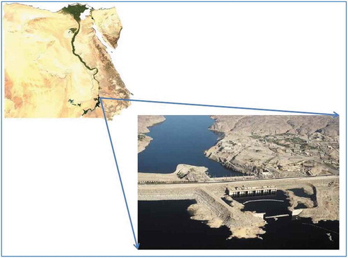
The operational strategy of the AHD is relatively complex compared with other dams worldwide (as it has extra storage consideration to maintain) and it is physically larger by capacity. In general, the reservoir inflow is one of the major factors affecting the operation rule for any dam. In this context, it is vital to have an accurate multi-lead-time inflow forecasting model for AHD reservoir in order to be able to optimize its operation rule. In 1959, an agreement between Egypt and Sudan was accepted, considering that the average annual Nile River flow at AHD is around 84 × 10⁹ m³ (billion cubic metres, BCM). Due to the location of the AHD in a relatively arid zone, the evaporation loss was estimated to be around 10 × 10⁹ m³ per year. Accordingly, the remaining 74 × 10⁹ m³ of water was split to allocate 55.5 and 18. × 10⁹ m³ to Egypt and Sudan, respectively.

The AHD is a rock-fill construction, which was built across the Nile River in the south of Egypt near the city of Aswan (almost 7 km), with a total length of 3.6 km, of which 0.52 km is between the Nile River banks, and the balance extends asymmetrically along both sides. For dam safety, a spillway was constructed on the western side of the dam. The height of the dam above the river bed is 111 m and the width at the bottom is 980 m. In order to minimize water seepage, there is a core of Aswan puddle clay, while the main materials used to build the dam body are sand and granite. The maximum reservoir water storage capacity is 162 × 10⁹ m³ (BCM)

Before the construction of the AHD, several studies were carried out in order to establish the natural inflow pattern at the location of the proposed dam. Based on natural inflow records for the period between 1871 and 1959, the annual average inflow of the Nile River at the AHD location was considered as very highly variable. The summary of the maximum, minimum and mean monthly inflow on a monthly basis, for the period 1959–2000 is presented in Table 1. In fact, the accuracy of flow records before the year 1900 has been criticized by various researchers owing to the fact that, during that period, the flow records were based on monitored water levels and adjusted rating curves to obtain the associated flow. However, these records are supported and verified by the records monitored at the Halfa gauge-station, south of the AHD, as well as the most recent flow records. Hurst et al. (1966) found that these records maintain the same mean and standard deviation (SD) statistics. To substantiate the statistical analysis of the inflow data at the AHD in the period 1871–2000, 20 sets of 100 annual Aswan flows were created and studied. It was observed that the mean ranged between 82 and 84 × 10⁹ m³, and the SD ranged between 18.1 and 19.3 × 10⁹ m³. These trials of analysis led to a high level of confidence in the data used in this study. We used actual natural inflow data, which cover 130 years of monthly Nile River flow data for the period 1871–2000. The monthly inflow data (in BCM) for the AHD are illustrated in Fig. 2. It can be observed that the Nile River has a natural hydrological regime that experiences both wet and dry seasons.

Table 1. Statistical analysis: maximum, minimum and average (mean) and standard deviation (SD) of the natural inflow at the AHD for the period 1870–2000.

Month	Maximum	Minimum	Mean	SD
	(10^9 m^3)	(10^9 m^3)	(10^9 m^3)	(10^9 m^3)
Aug.	29.10	6.50	18.96	4.50
Sep.	32.79	7.31	21.51	5.24
Oct.	27.40	5.97	14.52	4.40
Nov.	14.40	4.12	8.11	2.31
Dec.	11.00	2.83	5.54	1.45
Jan.	7.70	1.72	4.31	1.06
Feb.	6.04	1.15	3.16	0.94
Mar.	5.81	1.07	2.75	0.91
Apr.	5.26	0.95	2.52	1.07
May	4.72	0.80	2.33	1.03
Jun.	5.16	0.90	2.25	0.86
Jul.	11.03	1.74	5.24	1.84

Figure 2. Natural Nile River flow at Aswan High Dam: (a) time series of river flow, and (b) average of flow quantities for the period 1871–2000 on a monthly basis.

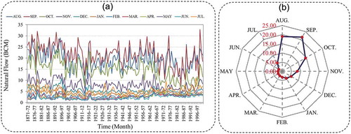
The first season is the flood season, which starts at the beginning of August and continues until almost the middle of November, while the second season is the dry spell which occurs during the rest of the year, between mid-November and the end of July. The maximum annual inflow may be seen for the water year 1877/78, with a volume of 150.33 × 10⁹ m³, and the minimum annual inflow occurred in the water year 1913/14,with a volume of 42.09 × 10⁹ m³. During the period 1870–2000, the mean annual inflow at the AHD was 91.2 × 10⁹ m³, and the SD was 19.13 × 10⁹ m³, which are relatively near to the results of Hurst et al. (1966). Finally, it may be seen that the largest ratio between the maximum and minimum inflow is nearly 6:1 in July, while the smallest, of almost 3:1, is in November.

In fact, one of the major reasons for selecting the AHD as a case study for this research was the need to examine the proposed models with highly stochastic, non-linear and complex consequences of the inflow, as seen in the Nile River. In addition, it is essential to develop an accurate multi-lead-time forecasting model in order to be able to generate optimal operation rules for the AHD to meet the demand patterns of the agricultural activities that mainly rely on the Nile River flow. It should be recalled here that, on an average, the agricultural water demand is about 46 × 10⁹ m³ a year, which is almost 83% of the total annual inflow of the Nile River.

3 Methodology

3.1 ANN

The artificial neural network (ANN) is a computational technique inspired by the idea to mimic the biological neural network in the human brain. The ANN consists of a set of nodes (neurons), which are placed in a number of layers. Each node in a layer receives and processes weighted input from the previous layer, and transmits to the output nodes through the subsequent layer links. Each link is assigned with a weight, which denotes its connection strength. The weighted summation of inputs to a node is converted to an output according to the selected transfer function (typically a sigmoid function) (Rezaie-Balf and Kisi 2018).

A multi-layer perceptron (MLP) is a class of feed-forward ANN, which is the most popular algorithm applied with a supervised learning technique called back-propagation for training (Graupe 2013). In this study, the MLP includes an input layer with each node of this layer representing an input variable, a hidden layer consisting of several hidden nodes, and an output layer representing the output variable used. Figure 3(a) shows the basic structure of the ANN model used for the forecasting of river inflow at the AHD. In the ANN model, input nodes are multiplied with assigned weights and then computed by a mathematical function (sigmoid, logistic sigmoid and hyperbolic tangent sigmoid), or activation function, which determines the activation of the neuron. These different artificial neurons are combined in order to process information and give the final output.

Figure 3. (a) Topological structure of the feed-forward neural network model, (b) schematic view of the M5 model tree (M5-MT), and (c) topological structure of the multivariate adaptive regression spline model (MARS).

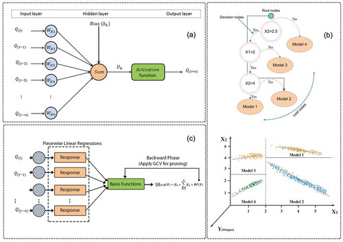
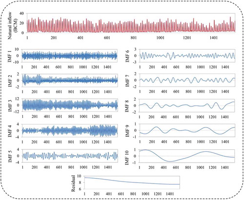
Figure 4. Time series data decomposition of reservoir inflow including high and low frequency values using the CEEMDAN method. BCM: billion cubic metres.

The number of hidden layers and the neurons in each layer along with the activation function affect the performance of the ANN (Wu et al. 2014). In this study, the optimum numbers of hidden layers and neurons in each hidden layer were found by a trial-and-error process. The hidden layers were varied from 1 to 3, and the neurons in each of them were varied from 2 to 15. Also, the sigmoid, logistic sigmoid and hyperbolic tangent sigmoid functions were examined to establish a suitable activation function. Additionally, the back-propagation algorithm, the commonly-used gradient descent optimization algorithm – with an adaptive learning rate of 0.45, momentum rate of 0.15, and learning cycle of 6000 – was applied to determine the weights and biases of the ANN. The performance of different models was compared.

3.2 M5-model tree (M5-MT)

The M5-MT was initially implemented by Quinlan (1992) to obtain a relationship between input–output parameters; it was reintroduced and improved by Wang and Witten (1996), who presented physically meaningful insights of certain phenomena. The M5 model can solve highly complex problems by dividing the data space into several sub-spaces (sub-problems) and build piecewise linear functions for each sub-domain at its terminal nodes. Therefore, the process of this algorithm is generally completed in two steps. In the first step, datasets are divided into subsets to construct an initial tree through a recursive splitting process. To determine the best attribute for splitting the dataset at each node, the standard deviation is used as a splitting criterion. Trees are constructed using the standard deviation reduction (SDR) schema, which maximizes the expected error reduction for each node as follows (Quinlan 1992):

(1) $\mathrm{S}\mathrm{D}\mathrm{R}=\mathrm{s}\mathrm{d}(I)-\sum _i\frac{\left|I_i\right|}{\left|I\right|}\mathrm{s}\mathrm{d}(I_i)$(1)

where I is the set of instances that reaches the leaf (node); I_i represents a subset of input data to the parent node; and sd is the standard deviation.

Secondly, after ‘pruning’ an over-grown tree, linear regression models are created and presented for each sub-tree of samples in the terminating nodes. The pruning process is performed to prune back the overgrown trees, which is a pivotal step to avoid the over-fitting problem and gain better generalization in the second stage. The sub-trees in this step are transformed into leaf nodes by replacing them with linear regression functions. Later, a smoothing procedure in which all the leaf models are amalgamated along the path back to the root is applied to realize a final model (Solomatine and Xue 2004, Bhattacharya and Solomatine 2005). For a better understanding of the M5-MT, a simple example of the general tree structure is presented in Fig. 3(b). As shown in Fig. 3(b), four linear regression models are built based on the tree-building process, and the structure of each sub-set is created by its knowledge. Thus, if X₁ < 2 and X₂ > 2.5, then the third model should be selected in the form $Y=a_o+a_1{X}_1+a_2{X}_2$, where a₀, a₁ and a₂ are regression coefficients, X_1, and X₂ are inputs and Y is the output. The reader is referred to Wang and Witten (1996) and Talebi et al. (2017) for more details on M5-MTs. In this study, the M5-MT was constructed using the WEKA 3.7 software and default parameters were employed in the model development stage.

3.3 Mars

Friedman (1991) pioneered multivariate adaptive regression splines (MARS) that belong to the category of non-parametric regression scheme capable and flexible of capturing all the inherent non-linear patterns present in the data to provide robust forecast results. The procedure involves splitting the predictor data into several units across the range of values and fitting linear regression models over each partition. In the course of the forward phase, the MARS algorithm explores for élite spots which are termed ‘knots’ to link two consecutive regression lines (functions) and the functions so fitted for each interval are termed “basis functions.” Every individual knot supports a couple of basis functions, which are usually two-sided truncated functions. The basis functions (BF) are generally expressed as:

(2) $\mathrm{B}\mathrm{F}1=max(0,c-x)$(2)

(3) $\mathrm{B}\mathrm{F}2=max(0,x-c)$(3)

where BF1 and BF2 are the basis functions, x is the predictor variable and c is a constant (threshold value) also referred to as knot. In the backward phase, by considering basis functions as standalone variables, the MARS algorithm constructs least-squares models which are subsequently pruned by eliminating additional knots taking into account the generalized cross-validation (GCV) criterion (Friedman and Roosen 1995). The model with the highest GCV is regarded to be the best MARS model.

The final form of MARS used to model the response variable is given by:

(4) $z=f(x)={\beta }_0+\sum _{p=1}^p{\beta }_p{K}_p(x)$(4)

(5) $\mathbb{Q}=\left\{{\left(x-c\right)}_{+},{(c-x)}_{+}\right\}$(5)

where β₀ is a constant, p is the number of basis functions, β_p is the coefficient of the pth basis function in the current model, K_p(x) denotes a basis function from set $\mathbb{Q}$, and the + signs assigned to the terms (x – c) and (c – x) indicate that only positive solutions are considered (Hastie et al. 2009). The mutual interactions among the BFs in the model are carefully considered when a new BF is added to the model space. BFs are added into the model to achieve the maximum specified number of terms that bring about a perfect fitness model. Thereafter, the backward pruning phase is applied to determine the best sub-models by pruning the number of knots; here, the less significant BFs having a lower impact on model efficiency are removed. The GCV criterion used to find optimal MARS model is expressed as (Zhang and Goh 2016):

(6) $\mathrm{G}\mathrm{C}\mathrm{V}=\frac{\mathrm{M}\mathrm{S}\mathrm{E}}{{\left[1-\frac{N+dN}{M}\right]}^2}$(6)

where M and N represent the number of observations and basis functions, respectively, MSE is the mean squared error and d refers to the penalty of each BF. Figure 3(c) shows the topological structure of the MARS model. For detailed information related to MARS and its algorithmic design, the reader is referred to StatSoft¹ and Milborrow (2018).

3.4 CEEMDAN

The complete ensemble empirical mode decomposition with adaptive noise (CEEMDAN) is an improved procedure of EEMD proposed by Wu and Huang (2009). The EEMD, which contains residual noise, poses adverse problems and also demands high computational cost. In this method, the number of sifting processes may increase the number of trials and various realizations of the signal; in addition, noise may build a different number of modes; consequently, it is difficult to calculate final averaging. In this regard, the CEEMDAN approach was developed to reduce the number of trials, while keeping the capacity to solve the mode mixing problem (Torres et al. 2011). CEEMDAN is a novel data pre-processing approach similar to EMD and EEMD and provides the following advantages: (1) An extra noise coefficient vector w is introduced to control the noise level at each decomposition; (2) reconstruction is complete and noise-free; and (3) it requires fewer trials than EEMD. The detailed steps of CEEMDAN analysis are:

Step 1. Use the same EEMD procedure to calculate the first mode function:

(7) $\overline{\mathrm{I}\mathrm{M}{\mathrm{F}}_1\left(t\right)}=\frac{1}{N}{\sum }_{j=1}^N{\mathrm{I}\mathrm{M}\mathrm{F}}_1^j\left(t\right)$(7)

Also, a unique first residue is then calculated as:

(8) $r_1\left(t\right)=x\left(t\right)-\overline{\mathrm{I}\mathrm{M}{\mathrm{F}}_1\left(t\right)}$(8)

Step 2. Define emd(t) as the kth IMF component by EMD, and then decompose the sequence r₁(t) + p₁emd₁(n_j(t)) to get the second IMF component by:

(9) $\overline{\mathrm{I}\mathrm{M}{\mathrm{F}}_2\left(t\right)}=\frac{1}{N}{\sum }_{j=1}^N\mathrm{e}\mathrm{m}{\mathrm{d}}_1\left[r_1\left(t\right)+p_1\mathrm{e}\mathrm{m}{\mathrm{d}}_1(n_j\left(t\right)\right]$(9)

The residual signal is:

(10) $r_2\left(t\right)=r_1\left(t\right)-\overline{\mathrm{I}\mathrm{M}{\mathrm{F}}_2\left(t\right)}$(10)

Step 3. Similar to the process in steps 1 and 2, the kth residual signal can be expressed by:

(11) $r_k\left(t\right)=r_{k-1}\left(t\right)-\overline{\mathrm{I}\mathrm{M}{\mathrm{F}}_k\left(t\right)}$(11)

and the k + 1th IMF component can be expressed as:

(12) $\overline{\mathrm{I}\mathrm{M}{\mathrm{F}}_{k+1}\left(t\right)}=\frac{1}{N}{\sum }_{j=1}^N\mathrm{e}\mathrm{m}{\mathrm{d}}_1\left[r_k\left(t\right)+p_k\mathrm{e}\mathrm{m}{\mathrm{d}}_k(n_j\left(t\right)\right]$(12)

Step 4. Repeat steps 1–3 until the residual signal meets the requirement of the termination criterion. Suppose there are L IMF components; then, the original sequence can be expressed by:

(13) $y\left(t\right)={\sum }_{i=1}^L\overline{\mathrm{I}\mathrm{M}{\mathrm{F}}_{\mathrm{i}}\left(t\right)}+r\left(t\right)$(13)

where r(t) is the final residual signal. In this study, the optimal standard deviation selected is 0.5, and the number of ensemble members was set to 500. Figure 4 presents the original river streamflow series decomposed by CEEMDAN. The authors used an open source Matlab code (Torres et al. 2011) of the CEEMDAN technique to decompose a hydrological time series.

3.5 Mallow’s c_p

In practical problems, there ar eseveral independent parameters, and the selection of the most influential parameters is a vital task for developing a robust forecasting model. The forecasting capability of the majority of AI-based approaches depends on optimal parameter subset selection (George 2000). For instance, the issue of subset selection comes into the picture when there is a number of predictors or highly correlated predictors for calibrating the predictive model, or when there is a redundancy among the independent parameters, which leads to multicollinearity (Fox 1991). There are some procedures to determine the best subset of predictors, such as stepwise methods: forward selection, backward deletion; Bayesian information criterion (BIC); Akaike information criterion (AIC) and the Mallow coefficient (C_p) (Cohen et al. 2014). Among them, the Mallow coefficient has been successful in choosing a minimum number of predictor variables for optimal model calibration. A small Mallow’s coefficient implies a good selection of predictor subset and a strong forecasting model. In the case of a specific problem, if among a set of k available predictors, p predictors are to be determined (k > p), the coefficient is calculated as (Mallows 1973):

(14) $C_p=\frac{\mathrm{R}\mathrm{S}{\mathrm{S}}_p}{\mathrm{M}\mathrm{S}{\mathrm{E}}_k}+2p-n$(14)

where RSS_p stands for the remaining sum of squares related to a model with p predictors, MSE_k is the mean squared error of regression model with the complete number of k predictors, and n is the sample size. Therefore, C_p indicates the mean squared error of a fitted model. The C_p compares the accuracy and bias of the fitted model with similar models fitted with a subset of the predictors (Kobayashi and Sakata 1990).

3.6 Model structure

In this study, to develop the ANN-, M5-MT- and MARS-based forecasting models of 1- to 6-month-ahead inflows of the AHD reservoir, the adequate lag or antecedent time values were considered as inputs. Determining effective input variables that have the highest impact on the output variable is a crucial step in developing robust predictive models. The characteristics of river flows cannot be distinguished accurately with a small number of input variables; similarly, an excessive number of input variables can cause model over-fitting problems (Rezaie-balf et al. 2017). Therefore, it is possible to represent the AHD reservoir inflow with antecedent values. First, inflow values with different lag times were considered as a base input structure.

(15) $D_{\left(t+n\right)}=f(D_{\left(t\right)},D_{\left(t-1\right)},D_{\left(t-2\right)},D_{\left(t-3\right)},D_{\left(t-4\right)},\dots ,D_{\left(t-15\right)}$(15)

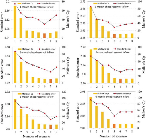
where t – 1, t – 2, t – 3 and t – 4 denote different monthly antecedent values of natural inflow time series (t), and n is the lead time number. To determine the most influential input variables for reservoir inflow forecasting at multiple lead-time, the Mallow C_p, a regression-based feature selection approach, was used. This was applied by sourcing the best subsets regression tool of Minitab software. Thereafter, the selected input variables were ready for the next phase.

To develop the decomposition-based models (CEEMDAN-based ANN, M5-MT and MARS models) which form the core objective of this study, the non-linear and non- stationary reservoir inflow time series dataset was divided into calibration and validation sub-sets and these were respectively decomposed into different components of IMFs along with one residual value included in the model input/output data series. The decomposition of the AHD reservoir inflow dataset into 10 IMFs, and one residual component is presented in Fig. 4. The three main process of the proposed CEMMDAN-based ANN, M5-MT and MARS models for reservoir inflow forecasting is as follows:

Step 1. To build an effective predictive model, the features of the original reservoir inflow datasets must be fully evaluated and considered. The data pre-processing approach based on the decomposition and ensemble strategy, CEEMDAN, is used to remove the noise and reduce the uncertainty of the original dataset, which is included as the input and output parameters. That is, the original reservoir inflow time series dataset y(t) (t = 1, 2, …, n) is decomposed into m IMF components c_i(t) (i = 1, 2, …, m), and a residual component r_m(t) using the CEEMDAN technique.

Step 2. Each proposed model as a forecasting tool is employed to predict each IMF extracted and residual components, separately, corresponding to each component.

Step 3. Finally, the obtained results using the models are combined to create a unit output which can be treated as the final forecasting results analogous to the original ones.

To summarize, despite the generalization ability of standalone models and due to the nonlinear and non-stationary nature of the hydrological time series, particularly reservoir inflow, it is necessary to search for alternative analyses to improve the accuracy of forecasting. In this regard, by using the CEEMDAN-based ANN, M5-MT and MARS models, which emphasize the ‘decomposition and ensemble’ idea, we aim to facilitate the forecasting process by dividing it into forecasting subtasks.

3.7 Model performance

The root mean square error (RMSE), normalized RMSE (NRMSE), normalized mean bias (NMB), Nash-Sutcliffe efficiency (NSE), normalized NSE (NNSE) and Willmott Index (WI) were used to evaluate the applied models. Their expressions may be expressed as follows:

(16) $\mathrm{R}\mathrm{M}\mathrm{S}\mathrm{E}=\sqrt{\frac{{\sum }_{i=1}^N{\left(Q_{i\mathrm{o}}-Q_{i\mathrm{o}}\right)}^2}{N}}$(16)

(17) $\mathrm{N}\mathrm{R}\mathrm{M}\mathrm{S}\mathrm{E}=\mathrm{R}\mathrm{M}\mathrm{S}\mathrm{E}/{\bar{Q}}_{\mathrm{o}}$(17)

(18) $\mathrm{N}\mathrm{M}\mathrm{B}=\frac{{\sum }_{i=1}^N\left(Q_{i\mathrm{m}}-Q_{i\mathrm{o}}\right)}{{\sum }_{i=1}^N{Q}_{i\mathrm{o}}}$(18)

(19) $\mathrm{N}\mathrm{S}\mathrm{E}=1-\frac{{\sum }_{i=1}^N{\left(Q_{i\mathrm{o}}-Q_{i\mathrm{m}}\right)}^2}{{\sum }_{i=1}^N{\left(Q_{i\mathrm{o}}-{\bar{Q}}_{\mathrm{o}}\right)}^2}$(19)

(20) $\mathrm{N}\mathrm{N}\mathrm{S}\mathrm{E}=\frac{1}{2-\mathrm{N}\mathrm{S}\mathrm{E}}$(20)

(21) $\mathrm{W}\mathrm{I}=1-\frac{{\sum }_{i=1}^N{\left(Q_{i\mathrm{o}}-Q_{i\mathrm{m}}\right)}^2}{{\sum }_{i=1}^N{(\left|Q_{i\mathrm{m}}-{\bar{Q}}_{\mathrm{o}}\right|+\left|Q_{i\mathrm{o}}-{\bar{Q}}_{\mathrm{o}}\right|)}^2}$(21)

where N is the number of used data, ${\bar{Q}}_{\mathrm{o}}$ is the mean value of the measured (observed) discharge, $Q_{i\mathrm{m}}$ is the calculated (modelled) discharge, and $Q_{i\mathrm{o}}$ is the measured discharge. For the ideal accuracy, the RMSE and MAE must be zero, while the NNSE and WI values must equal unity (Nash and Sutcliffe 1970, Willmott 1981, 1984).

In fact, to evaluate the performance of any forecasting model, a certain number of performance indicators (indices) should be calculated in order to designate its robustness in terms of error and accuracy dimension. By means of these indices, a comparitive analysis could be carried out in order to identify the best model among the proposed models. Six indices are calculated in this study to evaluate the performance of the proposed models. The RMSE statistic represents the measure of how the difference between the actual data and the model output is spread out. In addition, in some cases, there is a need to measure the error of the model without considering the absolute value of the error (ignorance of the error sign) in order to measure how the model output is biased; hence, the best performance index is the NMB (equation (18)). The NSE is a common index for measuring and weighing the prediction power of any forecasting model; its value can range between – ∞ and 1, and the closer the value of NSE to 1 the more accurate is the model performance for predicting the desired output. That is, the perfect match would be achieved when the value of NSE is equal to 1. Furthermore, the WI of agreement (equation (21)) judges how accurate the model output is relative to the actual data based on with pair-wise matched observations. Finally, in order to evaluate the performance of all the proposed models for the training or testing period, which are totally different in terms of the range of streamflow values (see Fig. 2), there is a need to select particular indices that may be used to provide a fair and unbiased measure of performance. Taking this into account, the RMSE and NSE indices were normalized to the mean of the observed data (NRMSE and NNSE).

4 Results and discussions

The reservoir inflows of the AHD were forecast 1 to 6 months ahead by implementing the AI tools ANN, MARS and M5-MT. To further improve the forecasting efficiency, hybrid AI models were developed using the data transformations afforded by the CEEMDAN technique as model inputs. Fot the multi-step-ahead forecasting task, the effect of stochastic time series components becomes more significant with the increase in lead time, which poses difficulty for identifying the number of significant lags of the variable(s) affecting the forecasting process. Hence, this study involved Mallow’s coefficient for the choice of minimum/optimal number of predictors (lags) for model development. The Mallow’s coefficient values for various input combinations used in this study are presented in Fig. 5. Various statistical measures, namely the RMSE, NRMSE, NMB, NSE, NNSE and WI (Sectoin 3.7) were considered for evaluating the accuracy of the inflow forecasting models. The performance statistics of both AI and hybrid-AI models pertaining to 1- to 6-month-ahead forecasts of the reservoir inflows are presented in Tables 2 and 3.

Table 2. Performance statistics of standalone and CEEMDAN-based ANN, MT and MARS models (1- to 3-step lead times).

	Training						Testing
	ANN	MT	MARS	CEEMDAN-ANN	CEEMDAN-MT	CEEMDAN-MARS	ANN	MT	MARS	CEEMDAN-ANN	CEEMDAN-MT	CEEMDAN-MARS
Q(t+1)
RMSE	1.7025	1.5586	1.5427	1.6663	1.5656	1.3319	2.0201	2.0043	1.7878	2.0357	1.9014	1.5616
RRMSE	0.2597	0.2378	0.2353	0.2542	0.2388	0.2032	0.2461	0.2442	0.2178	0.2480	0.2317	0.1903
NMB	0.0185	0.0009	0.0008	0.0132	0.0103	0.0111	–0.0223	–0.0733	–0.0214	–0.0282	–0.0275	–0.0012
NSE	0.9325	0.9434	0.9446	0.9353	0.9429	0.9587	0.9393	0.9402	0.9524	0.9383	0.9462	0.9637
NNSE	0.9368	0.9464	0.9475	0.9393	0.9460	0.9603	0.9427	0.9436	0.9546	0.9419	0.9489	0.9650
WI	0.9828	0.9852	0.9856	0.9833	0.9853	0.9895	0.9840	0.9833	0.9876	0.9846	0.9867	0.9912
Q(t+2)
RMSE	2.4275	2.0691	2.2039	2.0430	1.8127	1.5757	3.7233	2.8767	3.2208	2.3756	2.2380	1.7882
RRMSE	0.3704	0.3157	0.3362	0.3117	0.2766	0.2404	0.4559	0.3523	0.3944	0.2909	0.2741	0.2190
NMB	–0.0099	0.0005	0.0013	–0.0002	0.0008	0.0025	–0.0917	–0.1038	–0.1315	0.0413	0.0633	0.0295
NSE	0.8627	0.9003	0.8868	0.9028	0.9234	0.9422	0.7916	0.8756	0.8440	0.9152	0.9247	0.9519
NNSE	0.8793	0.9093	0.8983	0.9114	0.9289	0.9453	0.8275	0.8894	0.8651	0.9218	0.9300	0.9541
WI	0.9579	0.9730	0.9689	0.9738	0.9798	0.9851	0.9264	0.9619	0.9501	0.9756	0.9797	0.9873
Q(t+3)
RMSE	2.6632	2.2378	2.1966	2.1357	1.7383	1.6916	3.9530	3.1571	2.7521	2.5382	2.3124	1.9381
RRMSE	0.4064	0.3415	0.3352	0.3259	0.2653	0.2581	0.4844	0.3869	0.3373	0.3111	0.2834	0.2375
NMB	–0.0288	–0.0015	0.0014	–0.0002	0.0026	–0.0003	–0.1346	–0.1391	–0.1015	0.0513	0.0317	0.0543
NSE	0.8347	0.8833	0.8875	0.8937	0.9296	0.9333	0.7647	0.8499	0.8860	0.9030	0.9195	0.9434
NNSE	0.8581	0.8955	0.8989	0.9039	0.9342	0.9375	0.8095	0.8695	0.8976	0.9116	0.9255	0.9465
WI	0.9436	0.9679	0.9693	0.9707	0.9817	0.9826	0.9082	0.9515	0.9657	0.9749	0.9783	0.9855

Table 3. Performance statistics of standalone and CEEMDAN-based ANN, MT and MARS models (4- to 6-step lead times).

	Training						Testing
	ANN	MT	MARS	CEEMDAN-ANN	CEEMDAN-MT	CEEMDAN-MARS	ANN	MT	MARS	CEEMDAN-ANN	CEEMDAN-MT	CEEMDAN-MARS
Q(t + 4)
RMSE	2.5868	2.3589	2.2114	2.0208	1.5904	1.5831	3.7487	3.3445	3.0310	2.3628	2.4345	1.9784
RRMSE	0.3948	0.3600	0.3375	0.3084	0.2427	0.2416	0.4590	0.4095	0.3711	0.2893	0.2981	0.2422
NMB	–0.0932	–0.0003	0.0022	0.1045	–0.0016	–0.0024	–0.1639	–0.1589	–0.1285	0.0257	0.0446	0.0220
NSE	0.8440	0.8703	0.8860	0.9048	0.9410	0.9416	0.7888	0.8319	0.8619	0.9161	0.9109	0.9412
NNSE	0.8650	0.8852	0.8976	0.9131	0.9443	0.9448	0.8256	0.8561	0.8787	0.9226	0.9182	0.9444
WI	0.9511	0.9641	0.9687	0.9746	0.9846	0.9848	0.9233	0.9470	0.9569	0.9768	0.9761	0.9842
Q(t + 5)
RMSE	2.4003	2.3901	2.2520	2.1249	1.9957	1.7186	2.9010	3.3571	2.9488	2.5802	2.4233	1.9994
RRMSE	0.3664	0.3648	0.3437	0.3243	0.3046	0.2623	0.3549	0.4107	0.3607	0.3156	0.2964	0.2446
NMB	0.0020	–0.0003	0.0004	0.0010	0.0011	0.0030	–0.1246	–0.1528	–0.1038	0.0396	0.0545	0.0570
NSE	0.8656	0.8668	0.8817	0.8947	0.9071	0.9311	0.8737	0.8309	0.8696	0.9001	0.9119	0.9400
NNSE	0.8816	0.8824	0.8942	0.9047	0.9150	0.9356	0.8879	0.8554	0.8846	0.9092	0.9190	0.9434
WI	0.9653	0.9631	0.9674	0.9717	0.9754	0.9821	0.9616	0.9457	0.9595	0.9701	0.9748	0.9839
Q(t + 6)
RMSE	2.4408	2.4445	2.4525	2.1736	1.9858	1.8660	3.2172	3.4182	3.2371	2.3362	2.1471	2.0268
RRMSE	0.3722	0.3727	0.3740	0.3314	0.3028	0.2845	0.3933	0.4179	0.3958	0.2856	0.2625	0.2478
NMB	–0.0052	–0.0003	0.000001	–0.00001	–0.00001	0.0035	–0.1819	–0.1784	–0.1401	0.0364	0.0002	0.0225
NSE	0.8614	0.8609	0.8600	0.8901	0.9082	0.9190	0.8449	0.8249	0.8430	0.9182	0.9309	0.9384
NNSE	0.8782	0.8779	0.8772	0.9009	0.9159	0.9250	0.8657	0.8510	0.8643	0.9244	0.9354	0.9420
WI	0.9646	0.9613	0.9611	0.9701	0.9756	0.9786	0.9534	0.9438	0.9486	0.9763	0.9807	0.9833

Figure 5. Number of variables vs the minimum C_p and variance for 1-, 2-, 3-, 4-, 5- and 6-month-ahead flows.

4.1 Performance of standalone AI models

Employing diverse combinations of model parameters over several trail runs, the optimal ANN, MARS and M5-MT architectures were calibrated and accordingly tested for reservoir inflow forecasting of the AHD. Table 2 presents the performance indices (of both model training and testing phases) of ANN, MARS and M5-MT models designed for 1–3 steps-ahead forecasting. The one-step lead-time forecasting models are relatively superior, with smaller RMSE and NRMSE, and higher NSE, NNSE and WI compared to the two-step and three-step lead-time forecasting models.

The NMB statistic accounts for the proportionate differences in the observed vs simulated patterns of reservoir inflow. The computed NMB values signpost the generalized performance of the M5-MT and MARS models designed for 1- to 3-step-ahead forecasting. Overall, the M5-MT and MARS models gave reasonably acceptable inflow time series, with good performance indices, while forecasting up to 3 steps-ahed. The MARS model performance was superior to that of the M5-MT and ANN models with respect to various statistical indices in the case of 1- and 3-step-ahead forecasting. In the 2-step-ahead forecasting, however, the MARS model results were poor compared to the M5-MT model. In all three cases, the ANN is ranked as the worst in the reservoir inflow forecasting category.

Table 3 presents the performance indices (of both model training and testing phases) of the ANN, MARS and M5-MT models designed for 4- to 6-step-ahead reservoir inflow forecasting. The MARS model outperforms all other AI models in the 4-step lead time forecasting, while the ANN has slightly better accuracy than the MARS model in the case of 5- and 6-step-ahead forecasting. The NRMSE values of less than 0.4 during training and 0.45 during testing indicate relatively good performance of all the standalone models, even at 4- to 6-step-ahead forecasting. According to the NSE statistic, all the models show very good accuracy (NSE ˃ 0.750; Moriasi et al. 2007). The Willmott index (WI), which is a very sensitive indicator of extreme values, was found to be reasonably good for all lead time forecasts (Willmott et al. 2012).

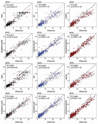
The scatterplots of standalone AI models of 1- and 2-step lead times are presented in the Appendix (Fig. A1). The one-step lead-time forecasts of the MARS model had regression fits with a coefficient of determination (R²) of 0.95, thus accounting for 95% of the variations in the test data. Its slope and bias coefficients are also closer to 1 and 0 compared to the M5-MT and ANN models. Among the 2-step lead-time standalone AI models, the M5-MT model accounted for 90.4% of variations in the test data, and its fit line is closer to the ideal line (y = x) compared to the MARS and ANN models. The MARS model accounted for 91.1% and 90.1% of variations in the test data, for 3-step and 4-step lead-time forecasting, respectively (Appendix, Fig. A2). The ANN model emerged as the most promising technique for forecasting higher lead-time reservoir inflows, providing forecasts that had reasonably good fits, with R² = 0.90 and 0.899 at Q(t + 5) and Q(t + 6) lead times, respectively, as evident from the scatterplots presented in Fig. A3. Although the MARS model has slightly lower R² than the ANN, the fit line of the latter model is closer to the ideal line. However, there is a slight difference between the MARS and ANN models at these two horizons, as may also be confirmed by the statistics given in Table 3. The MARS model can be considered as a better alternative to ANN because it has a less complex structure and provides explicit equations.

4.2 Performance of hybrid AI models

It is evident from both Tables 2 and 3 that the data transformations offered by CEEMDAN support performance improvement of the AI models. Among the 1-step lead-time models, the CEEMDAN-MARS model outperformed the others with less error (RMSE) and higher efficiency (NSE and WI) statistics during the test phase; improvements in RMSE are 23% and 18% compared to CEEMDAN-ANN and CEEMDAN-M5-MT. The CEEMDAN-MARS model improved the RMSE of the standalone MARS model by 12.65% during the test phase. In the case of 2- to 6-step lead-time models (Tables 2 and 3), the CEEMDAN-MARS model also provided relatively better forecasts than the other two hybrid models during testing. It may be observed that, during the test phase, the NRMSE statistic remains less than 0.25 in all 1- to 6-step lead-time CEEMDAN-MARS models, showcasing the robustness of the model forecasts. Overall, the CEEMDAN-MARS model provided relatively superior performance measures at all lead times during the test phase. Referring to the scatterplots presented in the Appendix (Fig. A1), it may be seen that the CEEMDAN-MARS model explains 96.8% and 95.3% of variations in the test data, for 1- and 2-step lead-time forecasting, respectively. The hybrid MARS model improved the standalone MARS model accuracy with respect to RMSE (45%, 30%, 35%, 32% and 37% for the 2- to 6-step-ahead forecasting of reservoir inflows, respectively). It is clear that the differences between the standalone MARS and hybrid MARS models are higher in the multi-step-ahead forecasting cases. This can also be observed for the other methods applied in this study. CEEMDAN-MARS respectively decreased the RMSE of CEEMDAN-ANN (CEEMDAN-M5-MT) by 25% (20%), 24% (16%), 16% (19%), 23% (18%) and 13% (6%), for 2- to 6-step-ahead forecasting. Referring to the scatterplots (Figs. A1 and A2) of the CEEMDAN-MARS model, the degree to which the dots are clustered in and around the best fit lines shows the generalization and robustness of the approach to forecast unseen/unlearned instances. Even at higher lead times – Q(t + 5) and Q(t + 6) – the CEEMDAN-MARS model was able to account for 94% of variations in the test data (Fig. A2). The non-dimensional and bounded composite measure, i.e. Willmott’s index of agreement was found to be greater than 0.98 in CEEMDAN-MARS models of all lead times thus portraying a perfect agreement between observed and forecasted values. During the test phase, the CEEMDAN-M5-MT models also provided reasonably accurate reservoir inflow forecasts with acceptable error measures up to two-step lead time. However, at higher lead times [Q(t + 3), Q(t + 4), & Q(t + 5)], the error statistic (RMSE) of CEEMDAN-M5-MT model was found to increase with decreasing model efficiencies. The six-step lead time CEEMDAN-M5-MT model yielded relatively similar performance to that of CEEMDAN-MARS model. This exposed the inconsistency & reliability of CEEMDAN-M5-MT model forecasts. Even though the CEEMDAN-ANN models were fairly accurate in terms of efficiency measures (NSE & WI), the error statistic (RMSE) and NMB measures were slightly loftier compared to the other hybrid AI models at all lead times during test phase.

4.3 Comparative evaluation of standalone and hybrid AI models

The scatterplots presented in Appendix 1, 2, and 3 serve as a better means for comparative evaluation of standalone and hybrid AI models. It could be observed that the forecast performance of each standalone model has been improved at all lead times with the support of CEEMDAN fostered data transformations as model inputs. The hybrid AI models have decent linear best fit lines compared to the standalone AI models at all lead times. The Taylor diagrams presented in Fig. 6 allows us to analyse the performance of all the models developed in terms of three statistical indices namely, the centered root mean square deviation (RMSD), correlation co-efficient (R) and standard deviation (σ). With reference to one-step lead time [Q(t + 1)] models, it could be noticed that the forecasts of CEEMDAN-AI models had (σ) clearly greater than the (σ) of the observed reservoir inflow categories.

Figure 6. Taylor diagrams of standalone and CEEMDAN-based models of (a) 1- and 2-step lead times; (b) 3- and 4-step lead times; and (c) 5- and 6-step lead times.

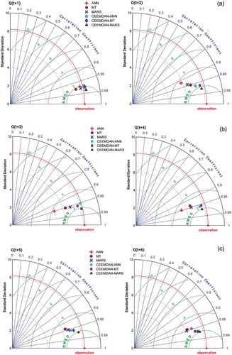
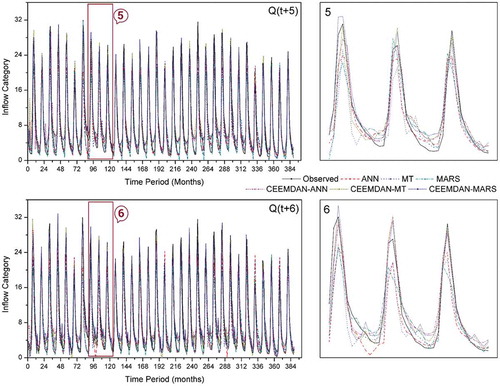
However, all the standalone AI models had offered forecasts in quite the opposite way. In the two-step lead time [Q(t + 2)] models, there exists clear cut evidence for inferior performance of standalone ANN model with a large magnitude of (σ) and relatively less R compared to CEEMDAN-MARS model (refer Fig. 6(a)). Similarly, the performance of standalone ANN model was the most inferior and CEEMDAN-MARS was the superior one among the Q(t + 3) and Q(t + 4) models (Fig. 6(b)). The standalone M5-MT model provided the most sub-par forecasts as per the Taylor diagram indices at Q(t + 5) and Q(t + 6) lead times (Fig. 6(c)). On the other hand, as per scatterplots (Fig. A1), the ANN models show inferior performance at Q(t + 5) and Q(t + 6) lead times. Based on Taylor diagrams plotted, the CEEMDAN-MARS model was found to provide optimal forecasts with relatively superior performance measures consistently, at all lead times. The time series plots of observed against forecasted reservoir inflows presented in Figs. 7, 8 and 9 depict the relative performance of each standalone and hybrid model in capturing the original/observed time series. The forecasts of hybrid AI models better followed the patterns of observed reservoir inflows compared to forecasts of standalone AI models. From the detailed graphs, considerable underestimation (overestimation) of the peak (low) flow values are clearly observed for the standalone models. The extreme values of the observed reservoir inflow time series were better accounted for by the CEEMDAN-MARS model at all lead times compared to the other models.

Figure 7. Reservoir inflow time series plots of standalone and CEEMDAN-based models 1- and 2-step lead times in the test period.

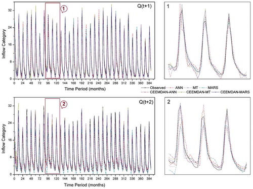
Figure 8. Reservoir inflow time series plots of standalone and CEEMDAN-based models of 3- and 4-step lead times in the test period.

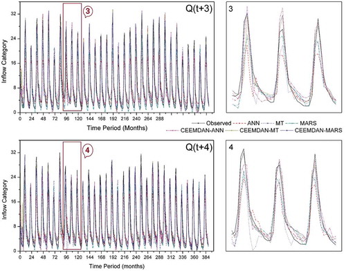
Figure 9. Reservoir inflow time series plots of standalone and CEEMDAN-based models of 5- and 6-step lead times in the test period.

5 Conclusions

The capability of new hybrid AI models to combine complete ensemble empirical mode decomposition with adaptive noise beside neural networks, multivariate adaptive regression splines and M5 model trees, was investigated in forecasting reservoir inflows of the Aswan High Dam. The most influencing input parameters of the applied models were decided according to Mallow’s coefficient (C_p). Among the standalone models, MARS performed well compared to the M5-MT and ANN models in 1- to 4-step-ahead forecasting. Although the ANN provided slightly better accuracy than the MARS model in 5- and 6-step-ahead forecasting, and it had the worst forecasts in the remaining cases (1- to 4-step lead times). Comparison of hybrid and standalone AI models based on the various statistics (RMSE, NRMSE, NMB, NSE, NNSE and WI) and comparing the figures (e.g. time variation graphs, scatterplots and Taylor diagrams) indicates superior accuracy of the hybrid models compared to the standalone ones. By combining with CEEMDAN, the RMSE of the ANN, M5-MT and MARS models was considerably improved, especially for forecasting multi-lead-time reservoir inflows. The RMSE increased by 36%, 36%, 37%, 11% and 27% for the ANN, by 22%, 27%, 27%, 28% and 37% for the M5-MT and 45%, 30%, 35%, 32% and 37% for the MARS models in 2-, 3-, 4-, 5- and 6-step lead time forecasting, respectively. Among the hybrid models, CEEMDAN-MARS outperformed the other models.

Although the proposed CEEMDAN-MARS model showed outstanding performance compared to the other models, it experienced a relatively negative feature that could be investigated and considered in future research, which is the time consumption for convergence during the training procedure. In fact, the convergence process during the training procedure is entirely slow, which is not ideal for real-time application. Therefore, it is recommended to investigate the potential for a similar accurate pre-processing method that could detect the highly non-linear and stochastic patterns in the data and, at the same time, could adapt the data in a much faster process. An alternative solution for such a negative feature could be achieved by integrating the CEEMDAN-MARS model with an optimization model that could speed-up the convergence process.

Disclosure statement

No potential conflict of interest was reported by the authors.

Additional information

Funding

This research was funded by the University of Malaya Research Grant (UMRG) coded RP025A-18SUS University of Malaya, Malaysia.

Notes

¹ http://www.statsoft.com/Textbook/Multivariate-Adaptive-Regression-Splines.

Appendix

Figure A1. Scatterplots of standalone and CEEMDAN-based models of one- and two-step lead times at AHD station.

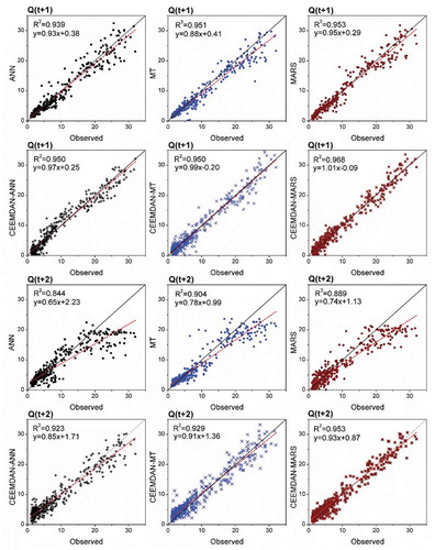
Figure A2. Scatterplots of standalone and CEEMDAN-based models of three- and four-step lead times at AHD station.

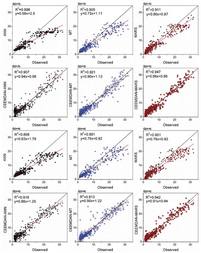
Figure A3. Scatterplots of standalone and CEEMDAN-based models of five- and six-step lead times at AHD station.

References

- Abudu, S., et al., 2010. Comparison of performance of statistical models in forecasting monthly streamflow of Kizil River, China. Water Science and Engineering, 3 (3), 269–281.
- Bhattacharya, B. and Solomatine, D.P., 2005. Neural networks and M5 model trees in modelling water level–discharge relationship. Neurocomputing, 63, 381–396. doi:10.1016/j.neucom.2004.04.016
- Can, I., Tosunoğlu, F., and Kahya, E., 2012. Daily streamflow modelling using ARMA and ANN models. Water Environment Journal, 26, 567–576. doi:10.1111/j.1747-6593.2012.00337
- Chu, H., Wei, J., and Qiu, J., 2018. Monthly streamflow forecasting using EEMD-Lasso-DBN method based on multi-scale predictors selection. Water, 10 (10), 1486. doi:10.3390/w10101486
- Clifford, N.J., et al., 2009. Numerical modeling of river flow for ecohydraulic applications: some experiences with velocity characterization in field and simulated data. Journal of Hydraulic Engineering, 136 (12), 1033–1041. doi:10.1061/(ASCE)HY.1943-7900.0000057
- Cohen, P., West, S.G., and Aiken, L.S., 2014. Applied multiple regression/correlation analysis for the behavioral sciences. New York: Psychology Press.
- Dobriyal, P., et al., 2017. A review of methods for monitoring streamflow for sustainable water resource management. Applied Water Science, 7 (6), 2617–2628. doi:10.1007/s13201-016-0488-y
- Fox, J., 1991. Regression diagnostics: an introduction. In: D. S. Foster, ed. Sage University paper series on quantitative applications in the social sciences. Newbury Park, CA: Sage, 07–079.
- Friedman, J.H., 1991. Multivariate adaptive regression splines. The Annals of Statistics, 19, 1–67. doi:10.1214/aos/1176347963
- Friedman, J.H. and Roosen, C.B., 1995. An introduction to multivariate adaptive regression splines. Statistical Methods in Medical Research, 4 (3), 197–217. doi:10.1177/096228029500400303
- George, E.I., 2000. The variable selection problem. Journal of the American Statistical Association, 95 (452), 1304–1308. doi:10.1080/01621459.2000.10474336
- Giupponi, C., et al., 2015. Integrated risk assessment of water-related disasters. In: J. F. Shroder, P. Paron and G. Di Baldassarre, eds. Hydro-meteorological hazards, risks and disasters. Netherlands: Elsevier, 163–200.
- Graupe, D., 2013. Principles of artificial neural networks. Vol. 7, Singapore: World Scientific.
- Hastie, T., Tibshirani, R., and Friedman, J., 2009. The elements of statistical learning. Springer series in statistics. New York, NY: Springer. http://link.springer.com/10.1007/978-0-387-84858-7.
- Honorato, A.G.D.S.M., Silva, G.B.L.D., and Guimarães Santos, C.A., 2018. Monthly streamflow forecasting using neuro-wavelet techniques and input analysis. Hydrological Sciences Journal, 63 (15–16), 2060–2075. doi:10.1080/02626667.2018.1552788
- Humphrey, G.B., et al., 2016. A hybrid approach to monthly streamflow forecasting: integrating hydrological model outputs into a Bayesian artificial neural network. Journal of Hydrology, 540, 623–640. doi:10.1016/j.jhydrol.2016.06.026
- Hurst, H.E., Black, R.P., and Simaika, Y.M., 1966. The major Nile projects. In: Cairo University, ed. The Nile Basin. Vol. X. Cairo, Egypt: Government Press.
- Kisi, O., 2007. Streamflow forecasting using different artificial neural network algorithms. Journal of Hydrologic Engineering, 12 (5), 532–539. doi:10.1061/(ASCE)1084-0699(2007)12:5(532)
- Kisi, O., 2009a. Wavelet regression model as an alternative to neural networks for monthly streamflow forecasting. Hydrological Processes, 23 (25), 3583–3597. doi:10.1002/hyp.7461
- Kisi, O., 2009b. Neural networks and wavelet conjunction model for intermittent streamflow forecasting. Journal of Hydrologic Engineering, 14 (8), 773–782. doi:10.1061/(ASCE)HE.1943-5584.0000053
- Kisi, O., 2015. Streamflow forecasting and estimation using least square support vector regression and adaptive neuro-fuzzy embedded fuzzy c-means clustering. Water Resources Management, 29 (14), 5109–5127. doi:10.1007/s11269-015-1107-7
- Kobayashi, M. and Sakata, S., 1990. Mallows’ Cp criterion and unbiasedness of model selection. Journal of Econometrics, 45 (3), 385–395. doi:10.1016/0304-4076(90)90006-F
- Mallows, C.L., 1973. Some comments on Cp. Technometrics, 15 (4), 661–675.
- Milborrow, S., 2018. Notes on the earth package. [online] http://www.milbo.org/doc/earth-notes.pdf [Accessed 8 August 2018]
- Mohammadi, K., Eslami, H.R., and Kahawita, R., 2006. Parameter estimation of an ARMA model for river flow forecasting using goal programming. Journal of Hydrology, 331 (1–2), 293–299. doi:10.1016/j.jhydrol.2006.05.017
- Moriasi, D.N., et al., 2007. Model evaluation guidelines for systematic quantification of accuracy in watershed simulations. Transactions of the American Society of Agricultural and Biological Engineers, 50, 885–900.
- Nash, J.E. and Sutcliffe, J.V., 1970. River flow forecasting through conceptual models part I—A discussion of principles. Journal of Hydrology, 10 (3), 282–290. doi:10.1016/0022-1694(70)90255-6
- Nwaogazie, I.L., 1987. Comparative analysis of some explicit-implicit streamflow models. Advances in Water Resources, 10 (2), 69–77. doi:10.1016/0309-1708(87)90011-X
- Quinlan, J.R., 1992, November. Learning with continuous classes. In: 5th Australian Joint Conference on Artificial IntelligenceIncorporating behaviour into animal movement modeling: a constrained agent based model for estimating visit probabilities in space-time prisms Hobart, Australia, vol. 92, 343–348.
- Regonda, S.K., Rajagopalan, B., and Clark, M., 2006. A new method to produce categorical streamflow forecasts. Water Resources Research, 42 (9), W09501. doi:10.1029/2006WR004984
- Rezaie-Balf, M. and Kisi, O., 2018. New formulation for forecasting streamflow: evolutionary polynomial regression vs. extreme learning machine. Hydrology Research, 49 (3), 939–953. doi:10.2166/nh.2017.283
- Rezaie-balf, M., et al., 2017. Wavelet coupled MARS and M5 model tree approaches for groundwater level forecasting. Journal of Hydrology, 553, 356–373. doi:10.1016/j.jhydrol.2017.08.006
- Rosenberg, E.A., Wood, A.W., and Steinemann, A.C., 2011. Statistical applications of physically based hydrologic models to seasonal streamflow forecasts. Water Resources Research, 47, W00H14. doi:10.1029/2010WR010101
- Shabri, A. and Suhartono, 2012. Streamflow forecasting using least-squares support vector machines. Hydrological Sciences Journal, 57 (7), 1275–1293. doi:10.1080/02626667.2012.714468
- Shiri, J. and Kisi, O., 2010. Short-term and long-term streamflow forecasting using a wavelet and neuro-fuzzy conjunction model. Journal of Hydrology, 394 (3–4), 486–493. doi:10.1016/j.jhydrol.2010.10.008
- Solomatine, D.P. and Xue, Y., 2004. M5 model trees and neural networks: application to flood forecasting in the upper reach of the Huai River in China. Journal of Hydrologic Engineering, 9 (6), 491–501. doi:10.1061/(ASCE)1084-0699(2004)9:6(491)
- Talebi, A., et al., 2017. Estimation of suspended sediment load using regression trees and model trees approaches (Case study: hyderabad drainage basin in Iran). ISH Journal of Hydraulic Engineering, 23 (2), 212–219. doi:10.1080/09715010.2016.1264894
- Torres, M.E., et al., 2011, May. A complete ensemble empirical mode decomposition with adaptive noise. In Acoustics, speech and signal processing (ICASSP), 2011 IEEE international Conference, Prague, Czech Republic. IEEE, 4144–4147.
- Vafakhah, M., 2012. Application of artificial neural networks and adaptive neuro-fuzzy inference system models to short-term streamflow forecasting. Canadian Journal of Civil Engineering, 39 (4), 402–414. doi:10.1139/l2012-011
- Vieux, B.E., Cui, Z., and Gaur, A., 2004. Evaluation of a physics-based distributed hydrologic model for flood forecasting. Journal of Hydrology, 298 (1–4), 155–177. doi:10.1016/j.jhydrol.2004.03.035
- Wang, Y. and Witten, I.H., 1996. Induction of model trees for predicting continuous classes. Waikato, New Zealand: The University of Waikato, Computer Science Working Paper 96/23.
- Wang, Z.Y., Qiu, J., and Li, F.F., 2018. Hybrid Models Combining EMD/EEMD and ARIMA for Long-Term Streamflow Forecasting. Water, 10 (7), 853. doi:10.3390/w10070853
- Willmott, C.J., 1981. On the validation of models. Physical Geography, 2 (2), 184–194. doi:10.1080/02723646.1981.10642213
- Willmott, C.J., Robeson, S.M., and Matsuura, K., 2012. A refined index of model performance. International Journal of Climatology, 32 (13), 2088–2094. doi:10.1002/joc.v32.13
- Willmott, H.C., 1984. Images and ideals of managerial work: a critical examination of conceptual and empirical accounts. Journal of Management Studies, 21 (3), 349–368. doi:10.1111/joms.1984.21.issue-3
- Wu, W., Dandy, G.C., and Maier, H.R., 2014. Protocol for developing ANN models and its application to the assessment of the quality of the ANN model development process in drinking water quality modelling. Environmental Modelling & Software, 54, 108–127. doi:10.1016/j.envsoft.2013.12.016
- Wu, Z. and Huang, N.E., 2009. Ensemble empirical mode decomposition: a noise-assisted data analysis method. Advances in Adaptive Data Analysis, 1 (01), 1–41. doi:10.1142/S1793536909000047
- Yaseen, Z.M., et al., 2015. Artificial intelligence based models for stream-flow forecasting: 2000–2015. Journal of Hydrology, 530, 829–844. doi:10.1016/j.jhydrol.2015.10.038
- Zhang, W. and Goh, A.T., 2016. Multivariate adaptive regression splines and neural network models for prediction of pile drivability. Geoscience Frontiers, 7 (1), 45–52. doi:10.1016/j.gsf.2014.10.003
- Zhang, Z., Zhang, Q., and Singh, V.P., 2018. Univariate streamflow forecasting using commonly used data-driven models: literature review and case study. Hydrological Sciences Journal, 63 (7), 1091–1111.