Groundwater contamination risks from conservative point source pollutants in a future climate

ABSTRACT

The groundwater contamination risk in future climates was investigated at three locations in Sweden. Solute transport penetration depths were simulated using the HYDRUS-1D model using historical data and an ensemble of climate projections including two global climate models (GCMs), three emission scenarios and one regional climate model. Most projections indicated increasing precipitation and evapotranspiration until mid-century with a further increase at end-century. Results showed both increasing and decreasing groundwater contamination risks depending on emission scenario and GCM. Generally, the groundwater contamination risk is likely to be unchanged until mid-century, but higher at the end of the century. Soil and site specific relationships between Δ(P – PET) (i.e. change in the difference between precipitation, P, and potential evapotranspiration, PET) and changes in solute transport depths were determined. Using this, changes in solute transport depths for other climate projections can be assessed.

KEYWORDS:

• climate change
• solute transport
• groundwater contamination
• HYDRUS-1D
• Sweden

Editor S. ArchfieldAssociate editor S. Huang

Introduction

The vadose zone acts as a filter, protecting ground water resources from pollutants spread on the soil surface. Assessing the risk for pollutants reaching the groundwater through the vadose zone is essential for protecting valuable groundwater resources. Pollutants can come from either point or diffuse sources. In very general terms, pollutants spread from non-point sources typically have lower concentrations and are less toxic compared to pollutants spread from point sources (e.g. Corwin 1996). Examples of point source pollutants are accidental spills of toxic substances, which are generally spread at relatively high concentrations over a limited area during a short period. Solute displacement through the unsaturated zone down to the groundwater is forced by infiltrated rainfall, snow melt or irrigation. The amount of excess precipitation (precipitation subtracted by actual evapotranspiration) and the temporal distribution of the precipitation will determine the depth of solute penetration, or the solute transport velocity. The intrinsic groundwater vulnerability depends on the likelihood of a pollutant reaching the groundwater due to the hydro-geological conditions. High solute transport velocities, or correspondingly, deep solute penetration depths, lead to an elevated risk for a pollutant spread at the soil surface to reach the groundwater table, thus increasing the vulnerability (e.g. Aller et al. 1987).

Several studies have confirmed the connection between high-intensity rainfall and macropore flow (e.g. Tiktak et al. 2004, Jarvis 2007, McGrath et al. 2010). Jarvis (2007) attributed this link to an enhanced macropore flow following high-intensity rainfall, by the ability of larger macropores to conduct water. Increasing rainfall intensity will lead to an increase also in pore water velocity, which in turn will reduce solute traveling time. It is obvious that rainfall intensity plays a key role in solute movement through macropores and that this process is well understood. Macropore flow is, undoubtedly, important in many soils. However, in soils with low clay content matrix flow still governs the solute movement process (Koestel and Jorda 2014). Also for matrix flow there is a connection between the temporal variability of infiltration and solute transport depths. This has been shown both experimentally and numerically (e.g. Persson and Saifadeen 2016). However, the connection between rainfall variability and solute transport velocities for matrix flow is not as straightforward as for macropore flow. For example, a low temporal variability (steady-state) irrigation can lead to faster solute transport velocities compared to intermittent irrigation (see, e.g. Sharma and Taniguchi 1991, Persson and Berndtsson 1999), but a high temporal variability of natural rainfall may also lead to faster transport (e.g. Bicki and Guo 1991, Persson and Saifadeen 2016). Thus, more research is needed in this field.

The predicted effects of climate change will lead to a changed risk for groundwater contamination. For example, global climate models (GCMs) predict a future change in the rainfall dynamics for many regions of the world with resulting higher maximum rainfall intensities, longer drought periods between rainfall events and a higher annual rainfall amount (IPCC 2013). In addition, changes in potential evapotranspiration will have a significant impact on soil water content dynamics and root water uptake rates. The predicted changes are likely to affect solute transport rates through the unsaturated zone. A logical way of assessing climate change impacts is using climate model output as input in water and solute transport models. However, there are only a few published studies that have estimated the change in solute transport (Arheimer et al. 2005, Olsson et al. 2016) or soil moisture distribution (Knapp et al. 2008, Gu and Riley 2010, Thomey et al. 2012; Stuart et al. 2012) for future rainfall climates. Knapp et al. (2008), based on both numerical and experimental results, concluded that future higher intensity rainfalls separated with longer dry periods would lead to a higher temporal variability of soil moisture in the top soil. This will, in turn, also affect solute transport velocities.

In order to accurately estimate the impacts of climate change on solute transport, detailed studies are required. For hydrological climate change impact assessment, a modelling scheme (or chain) has become state-of-the-art, where GCM output (mainly precipitation and temperature) is downscaled and bias adjusted, using dynamical and/or statistical approaches and subsequently used to force hydrological models (e.g. Olsson et al. 2016). In the present study, we adopt this approach for assessing the climate change impacts on solute transport, using the HYDRUS-1D (Šimůnek et al. 2016) as impact model. During the last decade, HYDRUS-1D has been widely used to simulate water flow and solute movement of different hypothetical and experimental problems with and without crops under different boundary conditions (e.g. Harman et al. 2011, Sutanto et al. 2012, Tafteh and Sepaskhah 2012, Wang et al. 2015, Dash et al. 2015, Selim et al. 2017).

In view of the above, the main goal of the present study is to investigate the effect of climate change on the movement of a conservative non-adsorbing solute in three different soil types cultivated by wheat in three different regions in Sweden. We believe that our study will lead to better understanding of the mechanism of solute dynamics through soil matrix under projected future climate and under the indirect effect of root water uptake. In addition, it will contribute towards a more complete picture of soil and groundwater sustainability in Sweden and other countries with similar conditions.

Materials and methods

Site descriptions

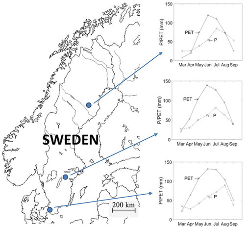
Three locations in Sweden were selected (Fig. 1): Malmö (55°34′17″N, 13°4′24″E), Norrköping (58°34′58″N, 16°8′49″E) and Petisträsk (64°34′1″N, 19°41′54″E) (the exact coordinates refer to the location of existing meteorological stations run by Swedish Meteorological and Hydrological Institute, SMHI). These locations were selected since they represent typical climate conditions for southern, middle (both with humid continental climate with cool summers) and northern (boreal climate) Sweden, respectively. At each site, three different soil profiles were considered. These profiles are three actual profiles situated close to Malmö. At each site the soil properties were measured every 0.1 m for the first meter and then every 0.5 m. The dominant soil layers were identified and the average soil properties were calculated for each layer. The soil types are referred to as sand, loam and clay according to FAO (2006) are presented in Table 1. Even though the profiles are actual profiles in southern Sweden, they represent typical agricultural soil types found in Sweden (and Northern Europe). The same profiles have also been used in previous studies (Persson and Saifadeen 2016, Selim et al. 2017).

Table 1. Soil properties, soil texture according to FAO (2006).

Soil type	Depth (cm)	Sand (%)	Silt (%)	Clay (%)	Bulk density (g/cm^3)
Sand	0–20	80	16.5	3.5	1.53
	20–45	78.8	18.3	2.9	1.55
	45–70	84.3	11.8	3.9	1.55
	>70	93.4	4.8	1.8	1.56
Loam	0–20	68.0	27.2	4.8	1.48
	20–150	58.2	33.0	8.9	1.48
	>150	40.5	44.6	14.9	1.65
Clay	0–120	59.0	25.6	15.4	1.45
	120–150	36.9	32.8	30.3	1.50
	>150	35.3	36.5	28.2	1.60

Figure 1. Locations of the three sites (from south to north): Malmö, Norrköping and Petisträsk, and the variation of P and PET between March and September.

Meteorological data

Historical observations

All meteorological data were collected by SMHI. Rain gauges used are of weighing type with a volume resolution of 0.1 mm (GEONOR A/S, Oslo, Norway). The original time resolution was 15 min, but in the present study 30 min accumulations were used. This type of rain gauges were installed in a national network in 1996. Available for the present study was a 20-year historical period (1996–2015) that was used as a climatological reference. The observations are subjected to careful quality control before being accepted in the SMHI data base and additional verification was performed during this study.

Potential evapotranspiration calculated using the Penman–Monteith equation (Allen et al. 1998) from meteorological measurements were also available for the stations on a monthly time step. The seasonal variation of precipitation (P) and potential evapotranspiration (PET) are similar for the three locations, but with higher PET in the south (especially in spring), reflecting higher temperatures (see Fig. 1).

Future projections

Future projections of precipitation were available from a limited ensemble of climate model simulations. Two GCMs were used – EC-Earth (Hazeleger et al. 2010) and CNRM (Voldoire et al. 2013) – each forced with two emission scenarios, i.e. representative concentration pathways (RCPs; Moss et al. 2008). The EC-Earth model was forced with RCP2.6 and RCP4.5, representing low and intermediate future emissions of greenhouse gases, respectively, whereas CNRM was forced with RCP4.5 and RCP8.5, where the latter represents high future emissions. We did this selection in order to cover a wide range of possible future climates covering the uncertainties coming from both the GCM and from the RCP. With the same RCP for both models, we would cover a smaller ‘RCP interval’. As RCP4.5 is considered a ‘medium scenario’, we included two simulations with this RCP. In the following, these combinations of GCMs and RCPs are called EC2.6, EC4.5, CNRM4.5 and CNRM8.5, respectively. These four future projections were dynamically downscaled to a spatial resolution of 11 km and temporal resolution of 30 min by the regional climate model (RCM) RCA4 (Kjellström et al. 2016). This resolution is among the higher in RCM projections, which often have a spatial resolution of 25–50 km and rarely an output time step below 1 day. The high resolution is expected to benefit in particular precipitation considering its extreme variability in both time and space.

It is well known that meteorological variables in general and precipitation in particular simulated by climate models are biased. If using the model output directly for subsequent modelling of, for example, hydrological impacts this bias may, at worst, lead to unrealistic results and erroneous conclusions (e.g. Yang et al. 2010). Therefore bias adjustment is a key component of the state-of-the-art modelling scheme mentioned in the introduction and it has evolved into a research field of its own (e.g. Maraun et al. 2015).

A way to ‘escape’ the issue of climate model bias is to employ the concept of delta change (DC; e.g. Hay et al. 2000). In DC, the climate model results are not used directly in the impact modelling but historical observations are statistically modified in order to reflect expected future changes (e.g. by increasing daily precipitation values by a certain percentage) and then these adjusted observations are used to represent future climate. Thus, no assessment is made of the climate model bias, i.e. to which degree the climate models can reproduce observations in a historical reference period, under the assumption that the accuracy of future changes is independent on historical agreement. This may be justified by the existence of climate variability as a key source of bias, i.e. the existence of bias does not necessarily imply that the climate model is inaccurate but rather that the simulation happens to be out-of-phase with low-frequency climate oscillations (e.g. Willems et al. 2012).

Delta change is commonly applied on a monthly time scale (e.g. Veijalainen et al. 2010). Thus, for each calendar month (e.g. May) a relative scaling factor (or DC factor) is estimated by dividing the May average value for a future time period in a climate projection with the May average in the same projection’s historical reference period. Then, this DC factor is applied to all May values in historical observations to produce a future realisation. When applied to precipitation this basic DC concept has some drawbacks, mainly that (i) the same adjustment is done for average values and extremes and (ii) changes in rainfall frequency (i.e. more or less wet time steps) are not considered.

Olsson et al. (2012) developed a DC version which uses high-resolution (sub-hourly) RCM results to overcome the above limitations. First of all, the DC factors are intensity-dependent, i.e. low and high precipitation intensities are adjusted separately. This makes it possible to reproduce rather complex future changes, such as lower summer totals but higher summer extremes, which are commonly found in climate projections (e.g. Olsson et al. 2009). Further, future changes in rainfall frequency may be realized through a procedure in which well-selected observed precipitation events are either removed or copied. See Olsson et al. (2012) for more details about the DC procedure.

In the DC application, three 30-year time slices were used for estimating future changes in rainfall statistics (to be transferred onto the historical time series) from the climate projections. In climate research, 30-year periods are common practice in order to get robust statistics with respect to future changes. The historical reference period (1986–2015) includes the 20-year period of the available observations, i.e. 1996–2015. It should be noted that the DC method used is designed to work with data of essentially arbitrary length (although the longer the better). Thus, the fact that the DC factors calculated using 30-year periods are applied to a 20-year periods of historical data is not an inconsistency, but fully in line with the methodology (see e.g. Olsson et al. 2012). Two future periods were used, one representing the middle of the current century (2031–2060) and one representing the end of the century (2071–2100). The relative changes between the reference period and the two future periods in all four RCM-projections were thus estimated and applied to the historical period, generating a total of eight future realizations of the precipitation at each site.

For running the solute transport model used we also need input of potential evapotranspiration. This variable is normally very uncertain in GCMs, even more uncertain than precipitation (see, e.g. Kay and Davies 2008). Attempts of using direct output led to unrealistic values (unrealistically high or low values and a very high variability). Instead, we used an ensemble average of nine GCMs to produce more robust estimates of monthly averaged potential evapotranspiration for each emission scenario (see Sjökvist et al. 2015). By comparing with monthly averaged evapotranspiration calculated by the same models for the historical period, DC factors for each emission scenario and future period were calculated. These DC factors were then applied to the evapotranspiration data series for the historical period to produce time series for the future scenarios. This gave stable and realistic evapotranspiration values, however, it also led to the values for the RCP4.5 scenario being identical for both GCMs.

HYDRUS model

System description

The domain geometry used to simulate solute transport under point source pollutant was one-dimensional (1D) and 2.50 m deep. The domain depth represents the typical depth of the ground water table in agricultural lands in Sweden. In total, 101 1D elements were used to discretize the simulation domain. The simulation domain was divided into sub-regions (four sub-regions in case of sand soil and three in case of loam and clay soils) to capture the variation in soil hydraulic properties throughout the simulation domain. Simulations of solute transport penetration were conducted yearly, the simulation period was 5000 h long, representing the period between 1 March and 25 September. The input time step of precipitation and evaporation was 0.5 h. This period represents approximately the growing season. By choosing this period we avoid problems with periods with below freezing temperatures and frozen soils.

Soil hydraulic parameters and solute parameters

Soil hydraulic parameters (Van Genuchten 1980) were estimated using the ROSETTA software package (Schaap et al. 2001), incorporated within HYDRUS-1D, using measured bulk density and percentages of sand, silt and clay (Table 2). Soil water hysteresis was considered, it was assumed that the α value for the drying curve was half the value of the wetting curve (e.g. Kool and Parker 1987, Selim et al. 2017). Solute parameters required during the present work were longitudinal dispersivity, molecular diffusion and adsorption isotherm coefficient. Longitudinal dispersivity was set to one-tenth of the profile depth (e.g. Anderson 1984, Cote et al. 2001). Molecular diffusion and adsorption were neglected during simulation.

Table 2. Soil hydraulic properties, parameters of the Van Genuchten (1980) model.

Soil type	Depth (cm)	${\theta }_r$	${\theta }_s$	Α (cm^−1)	n	Ks (cm/h)	$l$
Sand	0–20	0.0388	0.372	0.0437	1.818	5.011	0.5
	20–45	0.0369	0.3639	0.0457	1.769	4.374	0.5
	45–70	0.043	0.3709	0.402	2.081	7.01	0.5
	>70	0.0492	0.3677	0.034	3.255	24.16	0.5
Loam	0–20	0.0341	0.3714	0.0383	1.476	2.70	0.5
	20–150	0.0382	0.3683	0.024	1.432	1.53	0.5
	>150	0.0444	0.3334	0.0141	1.406	0.32	0.5
Clay	0–120	0.0518	0.3974	0.021	1.438	1.27	0.5
	120–150	0.0749	0.4078	0.0129	1.407	0.26	0.5
	>150	0.0682	0.3773	0.0127	1.384	0.16	0.5

Initial conditions

Based on a water table located 2.50 m below the soil surface, initial pressure head was assumed to vary linearly between 0 at the bottom edge of simulation domain to – 2.50 at the surface. The simulation domain was assumed to be initially free of pollutants except the top 5 cm, where 100 g of a non-absorbing conservative solute was uniformly distributed at the start of each modelling year (1 March). This scheme was selected as we wanted the solutes to be spread at the same circumstances every year and subsequent solute movement being only driven by the precipitation falling after the start of the simulation period.

Boundary conditions

As the water table is located 2.50 m below the soil surface, constant pressure head boundary conditions (BC) with a pressure head equal to zero was set at the lower edge of the simulation domain. Atmospheric BC, permitting for crop evapotranspiration (ETc), was set at the upper edge of the simulation domain. Spring wheat, which is among the most important agricultural crops in Sweden, was assumed to be grown during the period from the 29th of March to 5th of August in all simulation scenarios. In order to estimate ETc, the CROPWAT model (FAO 2012) was used to estimate daily reference crop evapotranspiration (ETo) based on the meteorological data. The collected meteorological data from Malmö, Norrköping and Petisträsk during the 20-year period from 1996 to 2015 was averaged on daily basis and used as input data for the CROPWAT model. Then, the calculated ET_o was multiplied by the crop coefficient for spring wheat to estimate daily ET_c. Each growing stage (i.e. initial, development, mid and late) was multiplied by the corresponding crop coefficient, K_c (Allen et al. 1998). The calculated ETc was used during the simulation of the historical period. By using the output of GCMs forced by different RCPs, the change in ET_c was calculated for each of the future climate projections. Daily values of ET_c were downscaled to a 0.5-h time step by assuming a sinusoidal variation between sunrise and sunset and evapotranspiration was neglected during the night. The HYDRUS-1D model do not use ET_c as input data, it instead considers evaporation (E) and transpiration (T) rates. To separate the calculated ET_c to E and T rates, the Belmans et al. (1983) equation for calculating E was used. The evaporation rate was estimated based on the leaf area index (LAI) and the extinction coefficient for solar radiation of 0.39 (Ritchie 1972). The WOFOST model (Boogaard et al. 1998) was used to calculate LAI for spring wheat during its different growth stages. For more details about calculation of ET_c and how to separate it into E and T, see Selim et al. (2017). The evaporation rate was set equal to ET_o during the period before and after the spring wheat growing date. During simulations, water ponding was allowed at the surface while surface runoff was neglected. Zero concentration gradient and concentration flux boundary conditions were assigned at the bottom and the top edges of simulation domain, respectively.

Root growth and root water uptake parameters

Root growth is determined based on the assumption that half of the rooting depth will be reached at the middle of the growing season (Šimůnek et al. 2008). In all simulation scenarios, the initial and maximum spring wheat rooting depths were set equal to 0.07 and 1.20 m, respectively (Zhou et al. 2012). Based on sowing and harvesting dates, the initial root growth and harvest times were assigned. To consider the effect of water deficit on root water uptake, the Feddes et al. (1978) model was used. This model is parameterized by four critical values of the water pressure head, h₃ < h₂ < h_opt< h_o describing plant stress due to dry and wet soil conditions:

(1) $\alpha \left(h\right)=\left\{\begin{array}{c}\frac{h-h_3}{h_2-h_3}{h}_2>h>h_3\\ 1h_{\mathrm{o}\mathrm{p}\mathrm{t}}>h>h_2\\ \frac{h-h_o}{h_{\mathrm{o}\mathrm{p}\mathrm{t}}-h_o}{h}_o>h>h_{\mathrm{o}\mathrm{p}\mathrm{t}}\\ 0h\ge h_{o}orh\le h_3\end{array}\right.$(1)

where h is the pressure head, h_o is the pressure head below which roots start to extract water from the soil, h_opt is the pressure head below which roots extract water at the maximum possible rate, h₂ is the limiting pressure head below which roots can no longer extract water at the maximum rate (and is a function of evaporative demand) and h₃ is the pressure head below which root water uptake ceases (the wilting point). In the HYDRUS model, two values, h_2H and h_2L related to higher and lower potential transpiration (r_2H and r_2L), respectively, should be set for h_2.

During simulation the following parameters were used; h_o = 0, h_opt = –1 cm, h_2H = –500 cm, h_2L = –900 cm, h₃ = –16,000, r_2H = 0.50 cm/h and r_2L = 0.1 cm/h. Salinity stress reduction effects were ignored during the simulations.

Solute transport for different climate scenarios

The solute distribution at the end of the 5000-h simulation period was estimated using HYDRUS-1D. In total 1620 simulations of solute displacement were conducted (20 years × 9 periods (1 historical and 8 future) × 3 soil types × 3 sites). In order to quantify the solute transport and to facilitate the comparison between different simulations, two variables to describe the solute displacement were calculated. These were; (i) the depth from the surface to the centre of mass of the solute, z_COM and the deepest depth where the concentration exceeded a given limit concentration, z_LC (in our case the limit was arbitrarily set to 0.2 g/L). These parameters represent the average and deepest solute transport, respectively. In order to investigate the significance of the difference between the z_COM and z_LC calculated using different rainfall data, the paired Student’s t-test was performed.

Results and discussion

Precipitation and evapotranspiration for different climate projections

A summary of the rainfall for the historical and future periods can be found in Table 3. The t-test showed that all changes in precipitation were significant at the p = 0.05 level, except EC2.6 at mid-century and EC4.5 at end-century in Malmö and Norrköping. Most projections predict an increase in precipitation to mid-century and a further increase to end-century. The only significant decrease in precipitation was predicted with EC2.6 in Malmö and Norrköping.

Table 3. Rainfall volumes (in mm) for different locations, periods and scenarios. The values are the average for the 5000-h periods studied each year during a 20-year period.

Source	Historical 1996–2015	Mid-century 2031–2050	End-century 2071–2090
Malmö
Measured	362
EC2.6		327	369
EC4.5		366	352
CNRM4.5		410	488
CNRM8.5		438	471
Norrköping
Measured	346
EC2.6		332	350
EC4.5		354	372
CNRM4.5		391	406
CNRM8.5		383	446
Petisträsk
Measured	349
EC2.6		356	374
EC4.5		414	463
CNRM4.5		385	431
CNRM8.5		369	449

Table 4 shows the future changes in some key precipitation characteristics during the studied period (March–September) as estimated from the climate projections. The future changes in both Malmö and Norrköping are consistently very small in the EC-Earth projections, whereas all metrics (average, maximum and frequency) exhibit a distinct increase in Petisträsk, most pronounced for RCP4.5 at end-century. In the CNRM projections there is a consistent and distinct increase in both average precipitation and precipitation frequency, whereas the increase in maximum precipitation is markedly lower and even negative (Petisträsk, mid-century).

Table 4. Future relative changes (%) in average, maximum and frequency of precipitation in the different locations and for different climate projections. Positive change indicates increasing values compared to the historical data.

Modell	RCP	Mid-century			End-century
		Average	Maximum	Frequency	Average	Maximum	Frequency
Malmö
EC-Earth	2.6	–6.0	6.1	–7.4	5.5	2.8	1.5
	4.5	–0.2	6.5	–4.3	–1.4	–0.6	–3.4
CNRM	4.5	13.7	7.1	10.4	36.2	9.4	26.7
	8.5	23.3	3.0	18.0	33.1	31.7	18.7
Norrköping
EC-Earth	2.6	3.6	–1.0	–1.6	3.8	0.6	–0.3
	4.5	0.4	2.2	–2.1	8.6	9.5	0.6
CNRM	4.5	11.4	16.1	10.0	17.7	7.0	15.2
	8.5	11.0	2.8	12.5	33.7	18.0	19.5
Petisträsk
EC-Earth	2.6	6.7	3.2	5.9	10.9	9.8	6.5
	4.5	15.6	15.2	7.6	34.4	17.2	22.5
CNRM	4.5	9.7	–10.9	11.9	26.5	3.6	23.1
	8.5	9.0	–1.8	10.4	40.3	1.1	35.5

In Malmö and Norrköping there is clearly a larger difference between the results from different GCMs than from different RCPs. The same tendency can be seen in Petisträsk, although less clear. It should be emphasized that the ensemble of projections spans a large range of different possible future changes, making it well suited for investigating possible impacts on solute transport.

The potential evapotranspiration (Table 5) also showed an increasing trend with time for all projections and locations, generally with higher increases in northern Sweden (Petisträsk). The total evapotranspiration was still clearly larger in Malmö than in Petisträsk, but the difference decreased, from around 40% in the historical period to around 30% at late-century. The net change in the difference between precipitation and potential evapotranspiration decreased in 75% of the future projections.

Table 5. Potential evaporation volumes (in mm) for different locations, periods and scenarios. The values are the average for the 5000-h periods studied each year during a 20-year period.

Source	Historical 1996–2015	Mid-century 2031–2050	End-century 2071–2090
Malmö
Measured	610
EC2.6		634	635
EC4.5		656	659
CNRM4.5		656	659
CNRM8.5		665	714
Norrköping
Measured	577
EC2.6		606	609
EC4.5		623	632
CNRM4.5		623	632
CNRM8.5		635	678
Petisträsk
Measured	433
EC2.6		472	475
EC4.5		503	507
CNRM4.5		503	507
CNRM8.5		509	541

Solute transport for different climate projections

Results in terms of z_COM and z_LC are presented as averages and standard deviation (SD) for each scenario, soil type and location are presented in Tables 6–11. In the tables, values indicating a significantly increased risk for groundwater contamination (or, equivalently, a higher solute transport velocity) are in bold while values indicating a significantly decreased risk for groundwater contamination are in italics.

Table 6. The average depth from the surface to the centre of mass of the solute, z_COM (in m) and the standard deviation (SD) for clay for different locations and time periods, and for different scenarios. Values in italics represent a significantly lowered risk for groundwater contamination and values in bold represent a significantly increased risk for groundwater contamination.

Source of input	Historical 1996–2015		Mid-century 2031–2050		End-century 2071–2090
	Average	SD	Average	SD	Average	SD
Malmö
Measured	0.360	0.150
EC2.6			0.327*	0.099	0.361	0.141
EC4.5			0.348*	0.150	0.332*	0.106
CNRM4.5			0.395**	0.166	0.502**	0.263
CNRM8.5			0.424**	0.187	0.441**	0.216
Norrköping
Measured	0.315	0.068
EC2.6			0.329	0.081	0.325	0.074
EC4.5			0.309	0.072	0.334	0.082
CNRM4.5			0.350*	0.094	0.342	0.084
CNRM8.5			0.328	0.080	0.367*	0.096
Petisträsk
Measured	0.445	0.144
EC2.6			0.429	0.141	0.458	0.160
EC4.5			0.499*	0.181	0.581**	0.198
CNRM4.5			0.443	0.147	0.516*	0.175
CNRM8.5			0.426	0.129	0.512*	0.163

*significant at the 0.05 level; **significant at the 0.01 level

Table 7. The average depth from the surface to the limit concentration of the solute, z_LC (in m) and the standard deviation (SD) for clay for different locations and time periods, and different scenarios. Values in italics represent a significantly lowered risk for groundwater contamination and values in bold represent a significantly increased risk for groundwater contamination.

Source of input	Historical 1996–2015		Mid-century 2031–2050		End-century 2071–2090
	Average	SD	Average	SD	Average	SD
Malmö
Measured	0.778	0.145
EC2.6			0.745*	0.120	0.788	0.140
EC4.5			0.767*	0.146	0.748**	0.131
CNRM4.5			0.804**	0.133	0.904**	0.164
CNRM8.5			0.853**	0.167	0.855**	0.160
Norrköping
Measured	0.775	0.077
EC2.6			0.758	0.062	0.760*	0.064
EC4.5			0.761	0.075	0.775	0.069
CNRM4.5			0.806*	0.086	0.803**	0.073
CNRM8.5			0.772	0.070	0.841**	0.082
Petisträsk
Measured	0.851	0.128
EC2.6			0.825	0.129	0.851	0.140
EC4.5			0.881	0.143	0.955**	0.137
CNRM4.5			0.830	0.130	0.894*	0.122
CNRM8.5			0.817*	0.123	0.896**	0.110

*significant at the 0.05 level; **significant at the 0.01 level.

Table 8. The average depth from the surface to the centRe of mass of the solute, z_COM (in m) and the standard deviation (SD) for loam for different locations and time periods, and different scenarios. Values in italics represent a significantly lowered risk for groundwater contamination and values in bold represent a significantly increased risk for groundwater contamination.

Source of input	Historical 1996–2015		Mid-century 2031–2050		End-century 2071–2090
	Average	SD	Average	SD	Average	SD
Malmö
Measured	0.381	0.170
EC2.6			0.346*	0.116	0.383	0.157
EC4.5			0.371	0.170	0.350*	0.124
CNRM4.5			0.426**	0.185	0.555**	0.294
CNRM8.5			0.460**	0.214	0.483**	0.257
Norrköping
Measured	0.339	0.077
EC2.6			0.345	0.096	0.344	0.086
EC4.5			0.326	0.085	0.366	0.094
CNRM4.5			0.387*	0.109	0.363	0.096
CNRM8.5			0.352	0.091	0.396*	0.114
Petisträsk
Measured	0.480	0.165
EC2.6			0.463	0.163	0.503	0.179
EC4.5			0.546*	0.208	0.647**	0.231
CNRM4.5			0.482	0.167	0.568**	0.200
CNRM8.5			0.462	0.145	0.567**	0.186

*significant at the 0.05 level; **significant at the 0.01 level.

Table 9. The average depth from the surface to the limit concentration of the solute, z_LC (in m) and the standard deviation (SD) for loam for different locations and time periods, and different scenarios. Values in italics represent a significantly lowered risk for groundwater contamination and values in bold represent a significantly increased risk for groundwater contamination.

Source of input	Historical 1996–2015		Mid-century 2031–2050		End-century 2071–2090
	Average	SD	Average	SD	Average	SD
Malmö
Measured	0.851	0.153
EC2.6			0.828*	0.136	0.861	0.151
EC4.5			0.838	0.154	0.829*	0.138
CNRM4.5			0.882**	0.160	1.001**	0.208
CNRM8.5			0.921**	0.179	0.932**	0.175
Norrköping
Measured	0.835	0.087
EC2.6			0.824	0.069	0.829	0.071
EC4.5			0.812**	0.078	0.847	0.077
CNRM4.5			0.888**	0.095	0.881**	0.077
CNRM8.5			0.839	0.078	0.921**	0.083
Petisträsk
Measured	0.926	0.149
EC2.6			0.910	0.152	0.958	0.166
EC4.5			0.971	0.163	1.031**	0.144
CNRM4.5			0.917	0.154	0.998**	0.161
CNRM8.5			0.903	0.138	0.998**	0.147

*significant at the 0.05 level; **significant at the 0.01 level.

Table 10. The average depth from the surface to the centre of mass of the solute, z_COM (in m) and the standard deviation (SD) for sand for different locations and time periods, and different scenarios. Values in italics represent a significantly lowered risk for groundwater contamination and values in bold represent a significantly increased risk for groundwater contamination.

Source of input	Historical 1996–2015		Mid-century 2031–2050		End-century 2071–2090
	Average	SD	Average	SD	Average	SD
Malmö
Measured	0.675	0.307
EC2.6			0.623*	0.261	0.686	0.302
EC4.5			0.645*	0.310	0.618*	0.277
CNRM4.5			0.734**	0.332	0.935**	0.429
CNRM8.5			0.815**	0.354	0.846**	0.385
Norrköping
Measured	0.609	0.176
EC2.6			0.613	0.184	0.613	0.155
EC4.5			0.568	0.154	0.638	0.163
CNRM4.5			0.711**	0.202	0.696*	0.177
CNRM8.5			0.625	0.170	0.769**	0.214
Petisträsk
Measured	0.813	0.314
EC2.6			0.799	0.312	0.857	0.324
EC4.5			0.939*	0.347	1.101**	0.346
CNRM4.5			0.832	0.319	0.990**	0.333
CNRM8.5			0.803	0.303	1.025**	0.327

*significant at the 0.05 level; **significant at the 0.01 level.

Table 11. The average depth from the surface to the limit concentration of the solute, z_LC (in m) and the standard deviation (SD) for sand for different locations and time periods, and different scenarios. Values in italics represent a significantly lowered risk for groundwater contamination and values in bold represent a significantly increased risk for groundwater contamination.

Source of input	Historical 1996–2015		Mid-century 2031–2050		End-century 2071–2090
	Average	SD	Average	SD	Average	SD
Malmö
Measured	1.472	0.511
EC2.6			1.429	0.480	1.512*	0.509
EC4.5			1.423*	0.512	1.419*	0.486
CNRM4.5			1.562**	0.495	1.784**	0.537
CNRM8.5			1.656**	0.501	1.705**	0.511
Norrköping
Measured	1.436	0.356
EC2.6			1.455	0.331	1.416	0.285
EC4.5			1.320	0.307	1.474	0.282
CNRM4.5			1.551	0.322	1.555*	0.303
CNRM8.5			1.430	0.293	1.713**	0.300
Petisträsk
Measured	1.615	0.431
EC2.6			1.624	0.436	1.689	0.440
EC4.5			1.780*	0.450	1.990**	0.419
CNRM4.5			1.642	0.432	1.855**	0.416
CNRM8.5			1.609	0.433	1.910**	0.399

*significant at the 0.05 level; **significant at the 0.01 level.

As the soil types are different in terms of soil texture, soil layering and initial water content profiles, different soil types should not be compared, but rather the same soil type at the different sites should be compared. However, some general differences between the different soil types could be pointed out. Both absolute and relative changes were larger in sand compared to clay, with loam in between. This would indicate that coarse textured soils are more sensitive to changes in precipitation compared to fine textured soils, but one should bear in mind that the differences were small. In general, both z_COM and z_LC behaved in a similar manner. For clay and loam the absolute changes in z_LC were similar to those for z_COM. For sand, on the other hand, the absolute changes in z_LC were larger than those for z_COM. Again, this implies that in course textured soils the groundwater contamination risk would increase more than in fine textured soils for a given increase in precipitation.

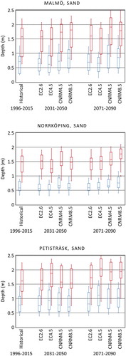
Results are also presented as box and whisker charts in Figs. 2–4 in order to display the variability of the data. From these figures, it can be seen that the variability in z_COM and z_LC is quite large. In general, variability was smaller in Norrköping, explained by the lower variability in precipitation for different years for this site (the standard deviations of the seasonal precipitation were 95, 44 and 79 mm for Malmö, Norrköping and Petisträsk, respectively). The standard deviation of z_COM was more or less unchanged for mid-century compared to the historical period, but increased for the end-century in all cases except for sand in Petisträsk. For the standard deviation of z_LC a small decrease until mid-century followed by an increase to end-century was found in Malmö, in the other locations the SD was more or less unchanged for mid-century and then decreased for end-century.

Figure 2. Box-and-whisker plots of z_COM (blue) and z_LC (red) for the three sites for clay. The horizontal line within each box shows the median, boundaries of the box indicate the 25th and 75th percentiles, and the whiskers indicate the highest and lowest values of the data series. Outliers are presented as circles.

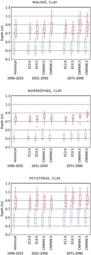
Figure 3. Box-and-whisker plots of z_COM (blue) and z_LC (red) for the three sites for loam. The horizontal line within each box shows the median, boundaries of the box indicate the 25th and 75th percentiles, and the whiskers indicate the highest and lowest values of the data series. Outliers are presented as circles.

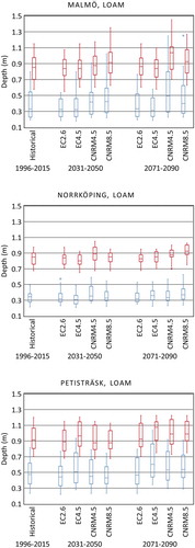
Figure 4. Box-and-whisker plots of z_COM (blue) and z_LC (red) for the three sites for sand. The horizontal line within each box shows the median, boundaries of the box indicate the 25th and 75th percentiles, and the whiskers indicate the highest and lowest values of the data series. Outliers are presented as circles.

Changes in average simulated solute transport depths for different projections compared to the historical period varied substantially, from –10% (Malmö, loam, EC2.6, mid-century) to +45% (Malmö, loam, CNRM4.5, end-century) for z_COM. It is interesting to compare the changes with the intra-annual variability of z_COM. One way of doing this is to compare the changes with the standard deviations of the z_COM for the historical periods. In all cases the absolute changes were smaller than the SD, however, the highest increases were almost as large as the SD. The changes in z_LC displayed a slightly smaller range compared to z_COM, from –8% (Norrköping, sand, EC4.5, mid-century) to +23% (Petisträsk, sand, EC4.5, end-century). The increases in z_COM and z_LC are related to increases in precipitation volume, wet fraction and increasing precipitation intensity. These parameters have also previously been shown to increase solute penetration depths (Persson and Saifadeen 2016).

In southern Sweden (Malmö) the CRNM model gave a significantly increasing groundwater contamination risk for both the RCP4.5 and RCP8.5 and both mid and end-century. In northern Sweden (Petisträsk), on the other hand, the CRNM model generally predicted an unchanged risk for mid-century and a significantly increasing groundwater contamination risk for end-century. The EC model generally gave unchanged or a decreasing risk in Malmö and Norrköping, while in Petisträsk results were mixed. Apparently, the generally increasing trends of both precipitation (P) and potential evapotranspiration (PET) seems to lead to an unchanged or increasing z_COM and z_LC in most cases. The largest solute transport depths were predicted when the increases in precipitation was higher than the increase in potential evapotranspiration.

One way of assessing the likelihood for changes in the groundwater contamination risk is by summarizing the results for all future scenarios in all soils. Doing this for mid-century, we found that 33, 50 and 17% of the scenarios showed an increasing, unchanged and decreasing z_COM, respectively. For the end of the century, the equivalent numbers were 53, 39 and 8%. If the same data were analysed separately for each soil type, we see that clay and loam behave the same, but the sand soil is slightly more prone to increasing z_COM for both mid and end-century. If we instead summarize the data for each location, we see a clear difference. In Malmö, 50, 0 and 50% of the scenarios showed an increasing, unchanged and decreasing z_COM, respectively, for mid-century. By the end of the century the corresponding values were 50, 25 and 25%. Thus, the changes were small and the number of scenarios giving an increased risk were not increasing. In Petisträsk, 0, 75 and 25% of the scenarios showed an increasing, unchanged and decreasing z_COM for mid-century, for the end-century these values changed to 75, 25 and 0%. Norrköping showed an intermediate pattern. In other words, the groundwater contamination risk seems to increase more for higher latitudes in Sweden.

In order to investigate the effects of changes in precipitation and potential evapotranspiration and its effects on solute transport we calculated the absolute change in the difference between seasonal P and PET, Δ(P – PET) as:

(2) $\mathrm{\Delta }\left(\mathrm{P}-\mathrm{P}\mathrm{E}\mathrm{T}\right)=\left(\mathrm{P}-\mathrm{P}\mathrm{E}\mathrm{T}\right)-\left(\overline{{\mathrm{P}}_{\mathrm{h}}}-\overline{\mathrm{P}\mathrm{E}{\mathrm{T}}_{\mathrm{h}}}\right)$(2)

where $\overline{P_h}$ and $\overline{\mathrm{P}\mathrm{E}{\mathrm{T}}_h}$ are the average seasonal precipitation and potential evapotranspiration for the historical period, respectively. Using Equation (2), a yearly value of Δ(P – PET) can be calculated, this was then compared to the absolute change in the difference between the yearly z_COM and z_LC calculated for the studied period and the average for the historical period; $\mathrm{\Delta }{z}_{\mathrm{C}\mathrm{O}\mathrm{M}}=z_{\mathrm{C}\mathrm{O}\mathrm{M}}-\overline{z_{\mathrm{C}\mathrm{O}\mathrm{M},\mathrm{h}}}$ and $\mathrm{\Delta }{z}_{\mathrm{L}\mathrm{C}}=z_{\mathrm{L}\mathrm{C}}-\overline{z_{\mathrm{L}\mathrm{C},\mathrm{h}}}$ respectively). In Fig. 5 we plot Δ(P – PET) against Δz_COM for sand in Malmö as an example. This was the location exhibiting most scatter, but still there is a clear trend between Δ(P – PET) and Δz_COM. In Fig. 5 a linear regression trend line (Δz_COM = 2.917Δ(P – PET) + 111.35, r² = 0.881) is also plotted. Plots of Δz_LC were similar, as were those for other sites and soil types. In all cases, a linear trend fitted the data well for small changes in Δ(P – PET). However, at high Δ(P – PET) (>250 mm) or low Δ(P – PET) (<–150 mm) the linear relationship underestimated Δz_COM slightly, especially for clay. Thus, care should be taken when applying the linear trend for predicting Δz_COM.

Figure 5. The absolute change in the difference between precipitation (P) and potential evapotranspiration (PET), Δ(P – PET) plotted against Δz_COM for the sand in Malmö (circles), along with $\mathrm{\Delta }\left(\bar{P}-\overline{\mathrm{P}\mathrm{E}\mathrm{T}}\right)$ plotted against $\mathrm{\Delta }\overline{z_{\mathrm{C}\mathrm{O}\mathrm{M}}}$ for the same dataset (crosses). The dotted line represents a linear regression for the Δ(P – PET) to Δz_COM relationship.

Similar to (2), changes in average P – PET can also be defined as one value for each future scenario:

(3) $\mathrm{\Delta }\left(\bar{\mathrm{P}}-\overline{\mathrm{P}\mathrm{E}\mathrm{T}}\right)=\left(\bar{\mathrm{P}}-\overline{\mathrm{P}\mathrm{E}\mathrm{T}}\right)-\left(\overline{{\mathrm{P}}_{\mathrm{h}}}-\overline{\mathrm{P}\mathrm{E}{\mathrm{T}}_{\mathrm{h}}}\right)$(3)

where $\bar{P}$ and $\overline{\mathrm{P}\mathrm{E}\mathrm{T}}$ are the average precipitation and potential evapotranspiration for the future scenario, respectively. Using Equation (3), $\mathrm{\Delta }\left(\bar{P}-\overline{\mathrm{P}\mathrm{E}\mathrm{T}}\right)$ can be calculated for each time period and can then be compared to the changes in the average z_COM and z_LC for each scenario and the average z_COM and z_LC for the historical period, e.g. $\mathrm{\Delta }\overline{z_{\mathrm{C}\mathrm{O}\mathrm{M}}}=\overline{z_{\mathrm{C}\mathrm{O}\mathrm{M}}}-\overline{z_{\mathrm{C}\mathrm{O}\mathrm{M},h}}$. It is interesting to observe that only one (out of 24) studied future scenarios had a significantly positive $\mathrm{\Delta }\left(\bar{P}-\overline{\mathrm{P}\mathrm{E}\mathrm{T}}\right)$ (p = 0.05), while 10–11 future scenarios (out of 24) had a significantly positive $\mathrm{\Delta }\overline{z_{\mathrm{C}\mathrm{O}\mathrm{M}}}$ for each soil type. In other words, even in situations where the PET increase more than P, the groundwater contamination risk might increase. One explanation could be the increase in the high intensity precipitation events, a parameter that previously have been shown to be positively correlated to solute transport depths (Persson and Saifadeen 2016, Selim et al. 2017). This also means that the choice of DC method is a key factor. It is important that the DC method accurately mimics the relevant statistical characteristics for future scenarios, not only for mean precipitation over a given time period, but also the magnitude and frequency of extreme events. One such example, also mentioned above, is that the GCMs can predict lower summer totals but higher summer extremes. This must be accurately described by the DC method.

One should bear in mind that the number of future projections was limited in the present study. However, the linear relationship between Δ(P – PET) and Δz_COM, could be used for calculating $\mathrm{\Delta }\overline{z_{\mathrm{C}\mathrm{O}\mathrm{M}}}$ for other scenarios with other values of $\bar{P}$ and $\overline{\mathrm{P}\mathrm{E}\mathrm{T}}$ . In Fig. 5 we show an example of this approach. In the figure the $\mathrm{\Delta }\left(\bar{P}-\overline{\mathrm{P}\mathrm{E}\mathrm{T}}\right)$ and $\mathrm{\Delta }\overline{z_{\mathrm{C}\mathrm{O}\mathrm{M}}}$ for the eight scenarios for Malmö, sand is plotted. As can be seen, these data points follow closely the linear relationship. In other words, the linear relationship between Δ(P – PET) and Δz_COM can be used to estimate $\mathrm{\Delta }\overline{z_{\mathrm{C}\mathrm{O}\mathrm{M}}}$ by calculating $\mathrm{\Delta }\left(\bar{P}-\overline{\mathrm{P}\mathrm{E}\mathrm{T}}\right)$ for other scenarios, at least as long as the $\bar{P}$ and $\overline{\mathrm{P}\mathrm{E}\mathrm{T}}$ values are within the ranges found in the present study.

Limitations and uncertainties

A study like the one presented here obviously has many uncertainties, in the emission scenarios, GCMs, RCM, DC method, solute transport model, etc. This needs to be taken into account when interpreting the results. The actual values of solute transport depths presented in the present study should not be overemphasized as no field validation of the model during a full season was conducted. Instead, the overall patterns of relative changes should be considered. As long as the uncertainties are kept in mind, we believe that our results can be used as a valuable guideline in assessing changes in the future groundwater contamination risk. Some specific limitations and their expected influence are discussed below.

Only non-adsorbing conservative solutes were considered in our study. A common example of such a pollutant is nitrate. Organic pollutants typically exhibits more or less strong sorption and will be transported slower. Our study can thus form a baseline for groundwater risk assessments. The modelling approach used in our study could also be extended to include both adsorption and degradation if the risks of a specific pollutant is to be assessed.

Our model only takes matrix flow into account. Especially in the clay soil macro pore flow is potentially of importance for a considerable amount of the solute transport. This means that the solute transport risk in clay soil might be underestimated in our study. Another limitation is that our model does not consider surface runoff and allowed for surface ponding. Surface runoff occurs when the rainfall intensity is larger than the infiltration capacity, which for saturated soils is equal to K_s. This do happen for a few 30-min time steps, but with only one exception, this never happens during two consecutive time steps. The exception was during one of the years during end-century in Malmö for CNRM8.5 in the clay soil, where the rainfall intensity was higher than K_s for two consecutive time steps. Since the agricultural land in Sweden is situated in plains with mild slopes, even if surface runoff is generated, most of it will be retained within the agricultural field to infiltrate as soon as the rainfall intensity decreases below K_s. Thus, surface ponding is expected to accurately model the actual real-world processes.

Due to the method chosen to handle evapotranspiration for the future scenarios, we were only able to produce one time series for each future period and RCP. This time series represents the average output of nine different climate models. In our study, the CNRM model consistently predicted higher temperatures compared to the EC model for the same RCP. This means that evapotranspiration probably was underestimated for the scenarios using rainfall input from the CNRM model and overestimated for the scenarios forced by the EC model. In turn, this would mean that solute transport depth is overestimated in the CNRM scenarios and underestimated in the EC scenarios.

Summary and conclusion

The groundwater contamination risk was assessed by simulating the transport depth at the end of the growing season for a conservative tracer added at the soil surface at the beginning of the growing season using HYDRUS-1D. The deeper (or equivalently, faster) the solutes are transported, the higher the risk for ground water contamination. Three different soil types at three different locations in Sweden were investigated. For each location and soil type, simulations were made for nine 20-year periods, one historical (1996–2015) and eight future projections. For the future projections, we used precipitation data from two GCMs using two RCPs each and two time periods representing mid- and late-century, respectively. Potential evapotranspiration used was calculated from an ensemble of nine GCMs for three emission scenarios.

Results showed that most future scenarios was predicted to have a significantly higher precipitation, up to 35% higher compared to the historical period. The potential evapotranspiration was predicted to increase with up to 25%. The net change in the difference between precipitation and potential evapotranspiration, however, decreased in 75% of the future projections.

Simulated solute transport depths varied substantially between different future projections, from – 10% to +45% for z_COM and – 8% to +23% for z_LC. Both the largest increases and decreases were found in southern Sweden. For mid-century, 33, 50 and 16% of the scenarios showed an increasing, unchanged and decreasing groundwater contamination risk, respectively. For the end of the century, the values were 53, 39 and 8%, respectively. In Malmö, the groundwater contamination risk will increase to the mid-century and the only increase slightly further for end-century. In Petisträsk, the groundwater contamination risk remains more or less unchanged until mid-century and then increase until end-century. There were only small differences between the soil types, however, sand showed a slightly higher likelihood of increased groundwater contamination risk in the future.

A high correlation between Δ(P – PET) (absolute change in the difference between precipitation (P) and potential evapotranspiration (PET)) and changes in z_COM and z_LC were found for each soil type and location.

One should note that the output of different GCMs, emission scenario and downscaling method result in very different values of z_COM and z_LC. The values presented here should be viewed as possible changes in z_COM and z_LC and results should not be considered to represent actual future changes. The derived relationships between Δ(P – PET) and changes in z_COM and z_LC could be used for estimation of solute transport depth changes for other future scenarios with other values of precipitation and potential evapotranspiration.

It should be noted that the results applies to conservative point source pollutions spread at the soil surface at the beginning of the growing season. A complete analysis of groundwater contamination risks would have to also involve the winter season with frozen soils and snow and snowmelt processes. This was, however, beyond the scope of the present study, but will be further investigated in the future.

Acknowledgements

The second author would like to thank the Egyptian Ministry of Higher Education for financing his stay at the Department of Water Resources Engineering, Lund University.

Disclosure statement

No potential conflict of interest was reported by the authors.

Additional information

Funding

Financial support was received from the Swedish Research Council Formas through projects HYDROIMPACTS 2.0 and SPEX.

References

- Allen, R., et al., 1998. Crop evapotranspiration, guidelines for computing crop water requirements. FAO irrigation and drainage paper No. 56. Rome, Italy: Food and Agriculture Organization of the United Nations.
- Aller, L., et al., 1987. DRASTIC: a standardised system for evaluating groundwater pollution potential using hydrogeologic settings. Ada, OK: US Environmental Protection Agency, EPA/60012-87/035.
- Anderson, M.P., 1984. Movement of contaminants in groundwater: groundwater transport advection and dispersion. In: National Research Council, ed. Groundwater contamination. Studies in geophysics. Washington, DC: National Academy, 37–45.
- Arheimer, B., et al., 2005. Climate change impact on water quality: model results from southern Sweden. AMBIO, 34, 559–566.
- Belmans, C., Wesseling, J.G., and Feddes, R.A., 1983. Simulation model of the water balance of a cropped soil: SWATER. Journal of Hydrology, 63, 271–286. doi:10.1016/0022-1694(83)90045-8
- Bicki, T.J. and Guo, L., 1991. Tillage and simulated rainfall intensity effect on bromide movement in an argiudoll. Soil Science Society of America Journal, 55, 794–799. doi:10.2136/sssaj1991.03615995005500030027x
- Boogaard, H., et al., 1998. WOFOST 7.1: user’s guide for the WOFOST 7.1 crop growth simulation model and WOFOST control center. Wageningen, The Netherlands: DLO Winand Staring Centre, Technical Report.
- Corwin, D.L., 1996. GIS applications of deterministic solute transport models for regional-scale assessment of non-point source pollutants in the vadose zone. In: D.L. Corwin and K. Loague, eds. Applications of GIS to the modeling of non-point source pollutants in the vadose zone. Madison, WI: Soil Science Society of America, SSSA Special Publication No. 48, 69–100.
- Cote, C.M., et al., 2001. Measurement of water and solute movement in large undisturbed soil cores: analysis of Macknade and Bundaderg data. CSIRO Land and Water, Technical Report 07/2001.
- Dash, J.C., et al., 2015. Prediction of root zone water and nitrogen balance in an irrigated rice field using a simulation model. Paddy Water Environment, 13, 281–290. doi:10.1007/s10333-014-0439-x
- FAO, 2006. Guidelines for soil description. 4th ed. Rome, Italy: Food and Agriculture Organization of the United Nations.
- FAO (Food and Agriculture Organization of the United Nations), 2012. FAO - water, natural resources and environment department [Online]. Available from: http://www.fao.org/land-water/databases-and-software/cropwat/en/ [Accessed 25 September 2019].
- Feddes, R.A., Kowalik, P.J., and Zaradny, H., 1978. Simulation of field water use and crop yield. New York, NY: John Wiley & Sons.
- Gu, C. and Riley, W.J., 2010. Combined effects of short term rainfall patterns and soil texture on soil nitrogen cycling - a modeling analysis. Journal of Contaminant Hydrology, 112, 141–154. doi:10.1016/j.jconhyd.2009.12.003
- Harman, C.J., et al., 2011. Climate, soil, and vegetation controls on the temporal variabilityof vadose zone transport. Water Resources Research, 47, W00J13. doi:10.1029/2010WR010194
- Hay, L.E., Wilby, R.L., and Leavesley, G.H., 2000. A comparison of delta change and downscaled GCM scenarios for three mountainous basins in the United States. JAWRA Journal of the American Water Resources Association, 36, 387–397. doi:10.1111/jawr.2000.36.issue-2
- Hazeleger, W., et al., 2010. EC-Earth. Bulletin of the American Meteorological Society, 91, 1357–1364. doi:10.1175/2010BAMS2877.1
- IPCC (Intergovernmental Panel on Climate Change), 2013. Climate change 2013: the physical science basis. Cambridge, UK and New York, NY: Cambridge University Press, Contribution of working group I to the fifth assessment report of the intergovernmental panel on climate change.
- Jarvis, N.J., 2007. A review of non-equilibrium water flow and solute transport in soil macropores: principles, controlling factors and consequences for water quality. European Journal of Soil Science, 58, 523–546. doi:10.1111/ejs.2007.58.issue-3
- Kay, A.L. and Davies, H.N., 2008. Calculating potential evaporation from climate model data: a source of uncertainty for hydrological climate change impacts. Journal of Hydrology, 358, 221–239. doi:10.1016/j.jhydrol.2008.06.005
- Kjellström, E., et al., 2016. Production and use of regional climate model projections – a Swedish perspective on building climate services. Climate Services, 2, 15–29. doi:10.1016/j.cliser.2016.06.004
- Knapp, A.K., et al., 2008. Consequences of more extreme precipitation regimes for terrestrial ecosystems. Bioscience, 58, 811–821. doi:10.1641/B580908
- Koestel, J. and Jorda, H., 2014. What determines the strength of preferential transport in Undisturbed soil under steady-state flow. Geoderma, 217–218, 144–160. doi:10.1016/j.geoderma.2013.11.009
- Kool, J.B. and Parker, J.C., 1987. Development and evaluation of closed-form expressions for hysteretic soil hydraulic properties. Water Resources Research, 23, 105–114. doi:10.1029/WR023i001p00105
- Maraun, D., et al., 2015. VALUE: a framework to validate downscaling approaches for climate change studies. Earth’s Future, 3, 1–14. doi:10.1002/2014EF000259
- McGrath, G.S., Hinz, C., and Sivapalan, M., 2010. Assessing the impact of regional rainfall variability on rapid pesticide leaching potential. Journal of Contaminant Hydrology, 113, 56–65. doi:10.1016/j.jconhyd.2009.12.007
- Moss, R.H., Nakicenovic, N., and O’Neill, B.C., 2008. Towards new scenarios for analysis of emissions, climate change, impacts, and response strategies. Geneva, Switzerland: IPCC. ISBN 978-92-9169-125-8.
- Olsson, J., et al., 2009. Applying climate model precipitation scenarios for urban hydrological assessment: a case study in Kalmar City, Sweden. Atmospheric Research, 92, 364–375. doi:10.1016/j.atmosres.2009.01.015
- Olsson, J., et al., 2012. Downscaling of short-term precipitation from regional climate models for sustainable urban planning. Sustainability, 4, 866–887. doi:10.3390/su4050866
- Olsson, J., et al., 2016. Hydrological climate change impact assessment at small and large scales: key messages from recent progress in Sweden. Climate, 4 (3), 39. doi:10.3390/cli4030039
- Persson, M. and Berndtsson, R., 1999. Water application frequency effects on steady state solute transport parameters. Journal of Hydrology, 225, 140–154. doi:10.1016/S0022-1694(99)00154-7
- Persson, M. and Saifadeen, A., 2016. Effects of hysteresis, rainfall dynamics, and temporal resolution of rainfall input data in solute transport modelling in uncropped soil. Hydrological Sciences Journal, 61 (5), 982–990.
- Ritchie, J.T., 1972. A model for predicting evaporation from a row crop with incomplete cover. Water Resources Research, 8 (5), 1204–1213. doi:10.1029/WR008i005p01204
- Schaap, M., Leij, F., and van Genuchten, M., 2001. ROSETTA: a computer program for estimating soil hydraulic properties with hierarchical pedotransfer functions. Journal of Hydrology, 251, 163–176. doi:10.1016/S0022-1694(01)00466-8
- Selim, T., Persson, M., and Olsson, J., 2017. Impact of spatial rainfall resolution on point source solute transport modelling. Hydrological Sciences Journal, 62 (16), 2587–2596. doi:10.1080/02626667.2017.1403029
- Sharma, M.L. and Taniguchi, M., 1991. Movement of a non-reactive solute tracer during steady and intermittent leaching. Journal of Hydrology, 128, 323–334. doi:10.1016/0022-1694(91)90145-8
- Šimůnek, J., et al., 2008. The HYDRUS-1D software package for simulating the movement of water, heat, and multiple solutes in variably saturated media, version 4.0: HYDRUS Software Series 3. University of California Riverside, Riverside, CA: Department of Environmental Science.
- Šimůnek, J., van Genuchten, M.T., and Šejna, M., 2016. Recent developments and applications of the HYDRUS computer software packages. Vadose Zone Journal, 15 (7), 25. doi:10.2136/vzj2016.04.0033
- Sjökvist, E., et al., 2015. Klimatscenarier för Sverige. Bearbetning av RCP-scenarier för meteorologiska och hydrologiska effektstudier. SMHI, Norrköping, Sweden: Klimatologi nr, 15.
- Stuart, M., et al., 2012. Review of risk from potential emerging contaminants in UK groundwater. Science of the Total Environment, 416, 1–21. doi:10.1016/j.scitotenv.2011.11.072
- Sutanto, S.J., et al., 2012. Partitioning of evaporation into transpiration, soil evaporation and interception: a comparison between isotope measurements and a HYDRUS-1D model. Hydrology and Earth System Sciences, 16, 2605–2616. doi:10.5194/hess-16-2605-2012
- Tafteh, A. and Sepaskhah, A.R., 2012. Application of HYDRUS-1D model for simulating water and nitrate leaching from continuous and alternate furrow irrigated rapeseed and maize fields. Agricultural Water Management, 113, 19–29. doi:10.1016/j.agwat.2012.06.011
- Thomey, M.L., et al., 2012. Effect of precipitation variability on net primary production and soil respiration in a Chihuahuan desert grassland. Global Change Biology, 17, 1505–1515. doi:10.1111/gcb.2011.17.issue-4
- Tiktak, A., et al., 2004. Assessment of the pesticide leaching risk at the pan-European level: the EuroPEARL approach. Journal of Hydrology, 289, 222–238. doi:10.1016/j.jhydrol.2003.11.030
- Van Genuchten, M.T., 1980. A closed-form equation for predicting the hydraulic conductivity of unsaturated soils 1. Soil Science Socitey of America Journal, 44 (5), 892–898. doi:10.2136/sssaj1980.03615995004400050002x
- Veijalainen, N., et al., 2010. National scale assessment of climate change impacts on flooding in Finland. Journal of Hydrology, 391, 333–350. doi:10.1016/j.jhydrol.2010.07.035
- Voldoire, A., et al., 2013. The CNRM-CM5.1 global climate model: description and basic evaluation. Climate Dynamics, 40, 2091–2121. doi:10.1007/s00382-011-1259-y
- Wang, X., et al., 2015. An assessment of irrigation practices: sprinkler irrigation of winter wheat in the North China plain. Agricultural Water Management, 159, 197–208. doi:10.1016/j.agwat.2015.06.011
- Willems, P., et al., 2012. Impacts of climate change on rainfall extremes and urban drainage systems. London, UK: IWA Publishing.
- Yang, W., et al., 2010. Distribution-based scaling to improve usability of regional climate model projections for hydrological climate change impact studies. Hydrology Research, 41, 211–229. doi:10.2166/nh.2010.004
- Zhou, J., et al., 2012. Numerical modeling of wheat irrigation using coupled HYDRUS and WOFOST models. Soil & Water Management & Conservation, 76 (2), 648–662.